Tourism and Economic Misery: Theory and Empirical Evidence from Mexico

Abstract

The misery index (MI) was devised to summarize the most evident costs for a society, attempting to objectively measure the loss in general welfare. It has been remarked in the literature that economic growth exerts a negative impact on the MI; however, analyses of this relationship in the tourism field have been neglected. This study assessed the effectiveness of the tourism sector at improving welfare conditions by measuring the impact of tourism GDP on the misery index and providing a theoretical framework for the relationship between tourism and the MI. A quantitative analysis was conducted using quarterly time series data for the period 2005Q1–2021Q2. Firstly, the existence of a long-term relationship was tested by using the Toda–Yamamoto procedure, and secondly, by applying linear and nonlinear ARDL models. The main results show that tourism can help to reduce the loss of welfare mirrored by the MI. These findings have policy implications, as they provide evidence that expanding the tourism sector counters the MI, and, consequently, the economic malaises derived from it.

1. Introduction

In recent years, many countries have experienced high inflation rates and relatively high unemployment. In this context, Okun’s misery index (MI), defined as the sum between unemployment and inflation, has resurged as a measure of interest (Clemens et al. 2022). The MI was conceived to measure economic dissatisfaction, attempting to summarize the most evident costs for society (Riascos 2009); therefore, despite its simplicity, it is considered an important criterion to quantify and monitor a population’s social welfare (Riascos 2009; Tule et al. 2017).

Over time, the MI has seen various applications; for example, Cakici and Zaremba (2023) found that the misery index is a reliable predictor of cross-sectional stock returns. For their part, Adrangi and Macri (2019) found that the MI has a statistically significant effect on the probability of approval of U.S. presidents’ performances. Meanwhile, Dadgar and Nazari (2018) found the existence of a negative relationship between economic growth and MI; they also found a statistically significant relationship between the index and government type. Moreover, authors such as Riascos (2009) and Grabia (2011) consider that the MI is a type of poverty index, although, according to Lechman (2009), Okun’s MI is not a perfect measure in this regard.

Tourism, for its part, is considered as helping to alleviate poverty by creating a vast number of jobs (Weinz and Servoz 2013). In fact, tourism has become a tool for alleviating poverty in ethnic areas by providing employment opportunities for residents (Wang and Lv 2023). Effectively, tourism is an important tool for creating employment and generating income; additionally, due to its intersectoral links, it can be considered an option for boosting development in regions where tourism activities can take place (Andrés-Rosales et al. 2023).

However, tourism is also considered a triggering factor for inflation in both the short and long term (Shaari et al. 2018). Tourism-led inflation usually occurs in goods and services such as public transport, shopping, culture and leisure, food services, and the different festivals and events that may take place in certain regions, although it can also be perceived in housing prices (Postma and Schmuecker 2017). Nonetheless, the tourism-led inflation phenomenon mostly occurs at the local level (Acerenza 2006), and it is often caused by demand pressures during high seasons (Kumar et al. 2015).

The above-mentioned observations imply that tourism has an opposite relationship with the components of the MI; on one hand, it reduces unemployment, but on the other hand, tourism can trigger inflation. In this sense, the objective of this study is to determine the relationship between tourism GDP and the MI. To achieve such an objective, a theoretical framework mostly based on Lovell and Tien’s (2000) observations on the MI is proposed, attempting to summarize the plausible effects of tourism on the MI. Secondly, a quantitative analysis based on Toda and Yamamoto’s (1995) test is performed to obtain evidence about the existence of a long-term relationship between the mentioned variables and its direction; afterward, linear and nonlinear Autoregressive Distributed Lag models, abbreviated as ARDL and NARDL, respectively, are applied to quantify the effects of tourism GDP on the MI in the form of elasticities. The empirical analysis is performed with quarterly data on the Mexican economy for the period 2005Q1–2021Q2.

Concerning the relationship between tourism and the MI, it is important to mention that Sánchez (2022a) found that, in the short term, international visitors, defined as the sum of international excursionists and tourists, have a negative effect on the compensated MI utilized by Hortalà and Rey (2011), which consists of subtracting the GDP growth rate from Okun’s MI. However, to the best of my knowledge, this is the first document analyzing the effect of tourism GDP on Okun’s MI and offering a theoretical framework on the relationship between such variables. Additionally, the findings of this work offer a clear vision of the positive effects of tourism for reducing the negative effects of the misery index.

The remainder of this document is organized as follows. The second section presents the literature review, which has been divided into two subsections; the first presents the relationship of tourism with employment and inflation, and the second develops the theoretical framework. The third section is also divided into two subsections; the first presents the data and their sources, and the second presents the models’ empirical design. The fourth section is also divided into two subsections; the first presents the Toda–Yamamoto test results, and the second presents those from the linear and nonlinear ARDL models. Finally, the discussion and conclusions are presented.

2. Literature Review

2.1. Tourism, Employment, and Inflation

Economic theory suggests that more production implies employing more workers; consequently, employment increases and unemployment falls (Tangarife 2013). However, it has been remarked in the literature that employment depends on more factors than just the production level, for instance, law, preferences, technology, social customs, and demographics (Neely 2010). Consequently, unemployment does not necessarily decrease in the same proportion that employment rises (Burggraeve et al. 2015). Effectively, in the case of Mexico, it has been found that the unemployment gap augments when the GDP growth rate falls under −1.01%, but superior GDP growth rates do not reduce such a gap (Loría and Salas 2022).

In tourism, employment demand is considered a function of the number of tourists, assuming that there is a positive relationship between tourist arrivals and employment demand (Walmsley 2017). Tourists’ spending is also considered an important item when analyzing tourism employment (Vanhove 1981), as the level of tourism employment depends on the demand for tourism goods and services (Tribe 2011).

Several documents have provided empirical evidence confirming the relationship between tourism and employment creation, claiming that tourism is an employment-intensive sector (Bhattarai et al. 2021). For example, in Slovenia, it was found that tourist arrivals exert a positive impact on the labor market (Rotar et al. 2023). It has also been proved that tourism demand has a positive effect on employment in countries such as Cyprus, Greece, Israel, Malta, and Tunisia (Yılancı and Kırca 2023). Similar evidence has been found in the case of the so-called “Emerging 7” economies (Zhao et al. 2023). Additionally, tourism creates numerous indirect jobs due to its intersectoral links (Acerenza 2006). Conversely, in Northern Portugal, inbound tourists have had a negative, although not statistically significant, impact on employment levels (Santos 2023).

In the case of Mexico, the palliative effect exerted by tourism on the unemployment rate has been empirically demonstrated by Loría et al. (2017) and Sánchez (2019), who modified the growth-rate version of Okun’s law. For their part, Alegre et al. (2019) showed that high unemployment rates can influence a person’s decision to travel, even if they are not out of the labor market, by augmenting their chances of not going on vacations. They remarked that this effect occurs when the unemployment rate surpasses 10%.

Inflation, for its part, is an economic phenomenon that has traditionally been defined from two equivalent perspectives; on one hand, it can be viewed as a process in which prices continuously rise, while, on the other hand, it can be considered a process in which money constantly loses its value (Frisch 1983). Inflation plays an important role in determining the degree of trade openness, which is one of the main drivers of economic growth (Khan et al. 2023). Tourism, for its part, is considered an important activity in determining inflation in both the short and long term (Shaari et al. 2018), and tourism inflationary pressure is frequently caused either by increases in tourism demand or high production costs (Mihalič 2014).

It has been noticed that tourism mainly contributes to inflation by increasing the prices of food and drink products, entertainment, transport, and services (Kumar et al. 2015), as well as by elevating both rent costs and land value. Although the latter two effects could be beneficial for property owners, they could cause problems for those residents wanting to buy or rent a property (Frent 2016). In the case of the Barbadian economy, it has been observed that tourists “compete with locals for available consumption and infrastructural goods”, so tourism exerts upward pressure on prices, particularly in sectors where supply cannot be adequately adjusted in the short term (Coppin 1993). Additionally, tourists usually have more purchasing power than residents; therefore, while tourists can deal with high prices, residents’ welfare diminishes, as they have to use the same providers (Sancho 1998). Additionally, supplementary charges may be imposed on residents to finance tourist venues (Kumar et al. 2015).

It is important to mention that tourism-led inflation usually takes place at the local level, although the inflationary pressure exerted by tourism can extend nationwide (Acerenza 2006). In the same vein, as tourism inflation is usually induced by increased demand, it frequently occurs during the high season (Kumar et al. 2015). For example, in Mexico, during July 2022, the increase in tourist package prices doubled the general year-on-year inflation rate (Castillo 2022).

As reported by Castillo (2022), inflationary pressure elevates tourists’ average spending. Nonetheless, price increases normally lower demand (Varian 1999), especially in sectors such as tourism where demand is highly sensitive to price variations (Sancho 1998). Effectively, in the case of Indonesia, it has been found that inflation has a negative impact on international tourist arrivals (Sulasmiyati 2018). Meanwhile, in Mexico, high inflation rates have slowed down investment in tourism due to increases in the cost of water, electricity, and fuel (Forbes Staff 2022).

Figure 1 summarizes the information provided in this section: on one hand, tourism increases inflation, at least at the local level, but, on the other hand, inflation reduces tourism. This figure also illustrates the existence of a reinforcing negative effect between tourism and unemployment in the sense that tourism reduces unemployment but unemployment reduces tourism.

Concerning the relationship between tourism and the MI, as mentioned before, Sánchez (2022a) found that international visitors have had a negative impact on the compensated misery index utilized by Hortalà and Rey (2011). However, the nature of the relationship between tourism GDP and Okun’s MI is not clear.

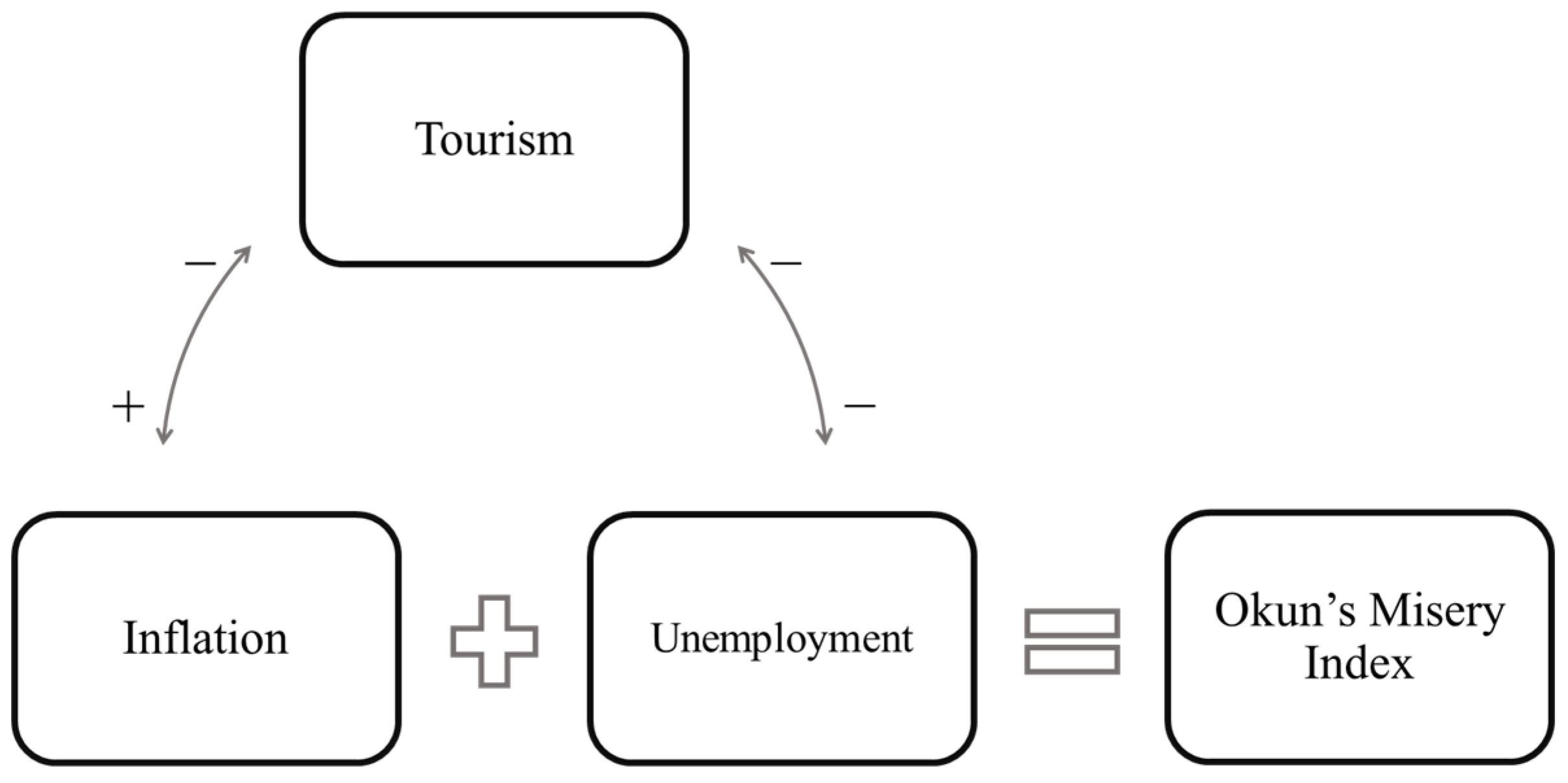
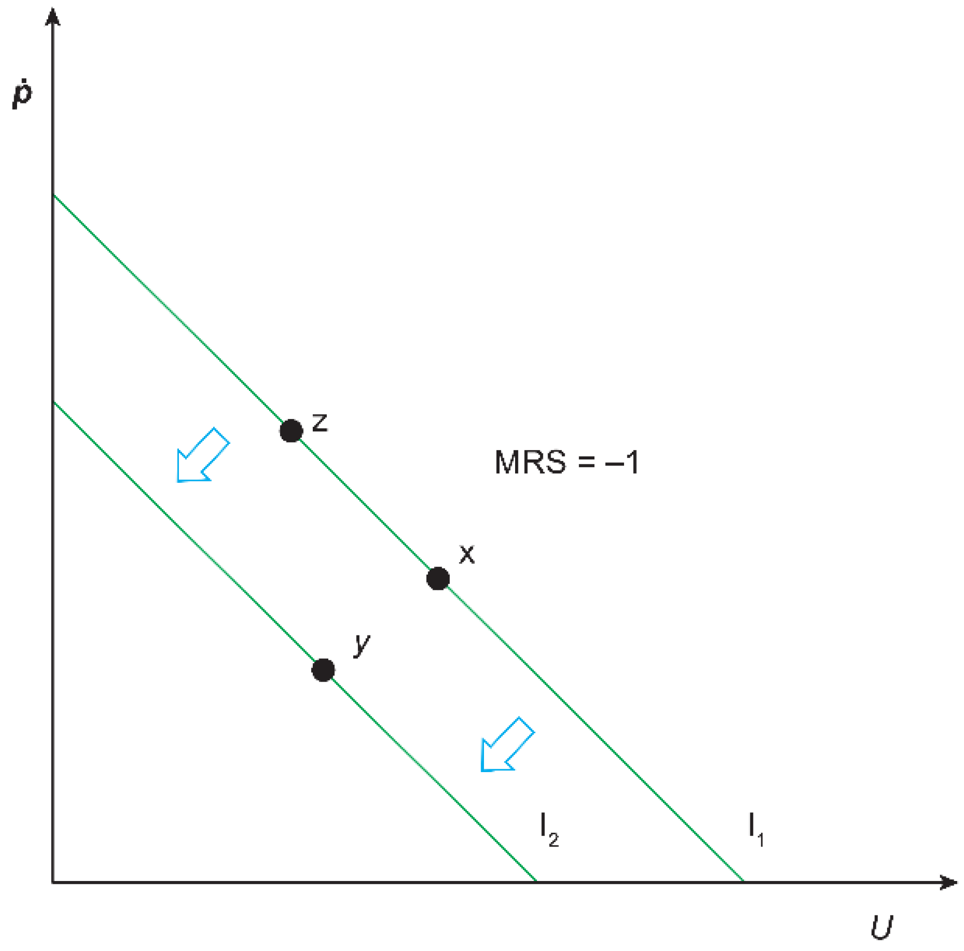
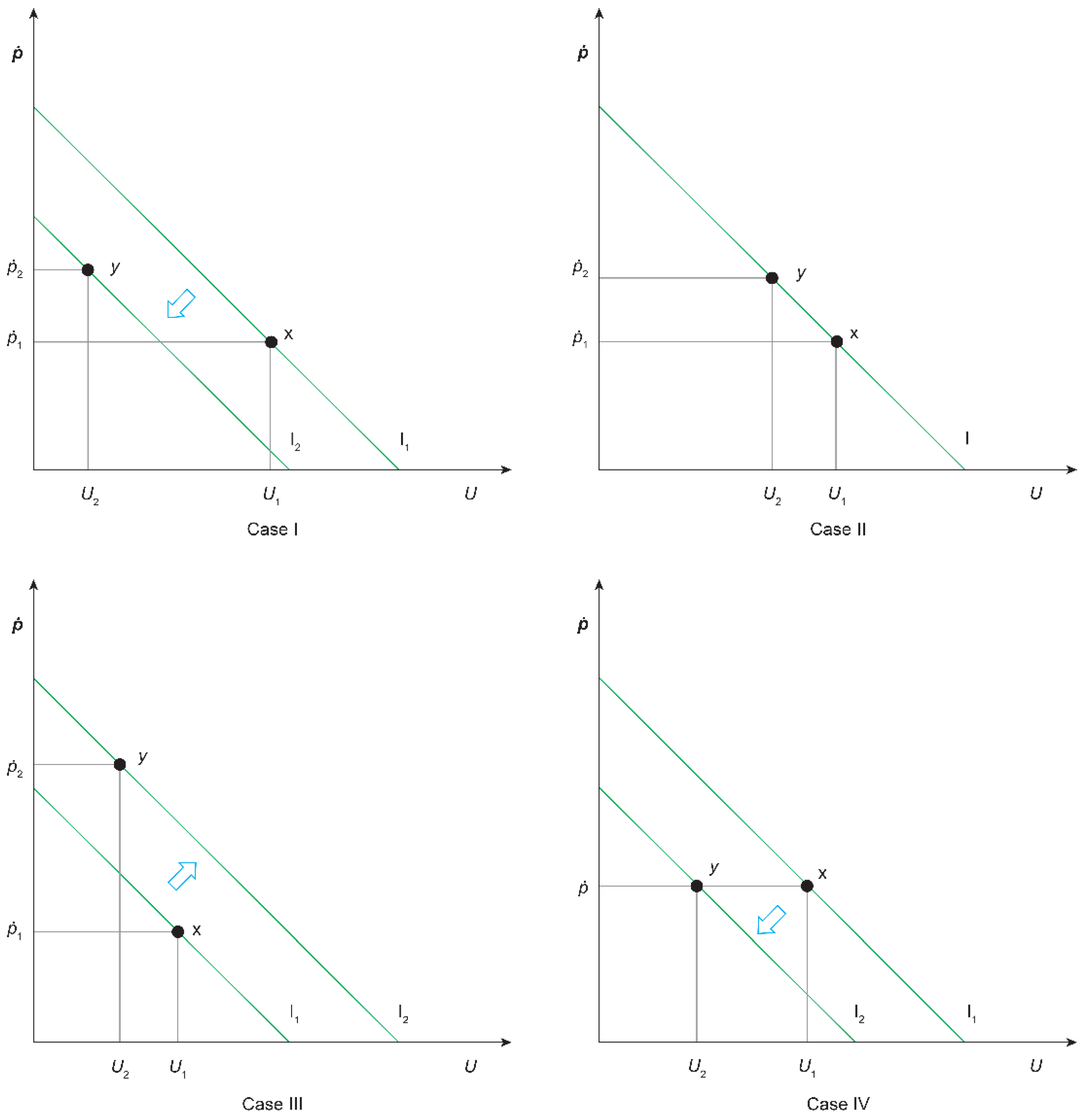
2.2. Misery Index and Tourism: A Theoretical Approach

The MI was devised by the economist Arthur Okun in the 1970s, when most of the world was undergoing high inflation and unemployment rates (Nessen 2008). This indicator, also known as the economic discomfort index, was probably the first attempt to summarize the macroeconomic performance during the business cycle in a single number (Cohen et al. 2014). The MI is defined as the unweighted sum of unemployment and inflation rates (Cohen et al. 2014; Dornbusch et al. 2002; Tule et al. 2017). In Equation (1), following Sánchez (2022a), $U$ represents the unemployment rate and $\dot{p}$ represents the inflation rate:

$$Okun’s Misery Index=\dot{p}+U$$

(1)

Unemployment and inflation are decisive macroeconomic variables for determining a nation’s social and economic welfare. They are indispensable indicators for assessing the economic policy success (Masárová et al. 2022). In fact, Lechman (2009) considers that the MI, despite being rudimentary, is a good proxy for measuring economic and social welfare, as its variations reflect society’s economic performance. Additionally, Di Tella et al. (2001) found that both unemployment and inflation are highly correlated with social well-being, although life satisfaction is not entirely captured by the linear misery function defined in Equation (1).

Given that Okun’s MI only takes two macroeconomic indicators into account, Lovell and Tien (2000) consider that it can be interpreted as a “crude (dis)utility function”, in which indifference curves are straight lines with a marginal rate of substitution, ($MRS$), equal to −1. This implies that individuals feel exactly the same aversion to both unemployment and inflation, as per Varian (1999), assuming that $MRS=-1$ corresponds to the simplest case of perfect substitutes.

Following the above-mentioned remarks, Figure 2 displays the indifference curves for Okun’s MI. As inflation and unemployment reduce well-being (Blanchflower et al. 2014), it should be the case that basket $\mathrm{y}$ is strictly preferred over basket $\mathrm{x}$. As both inflation and unemployment are bads, economic discomfort should decrease as the levels of these two macroeconomic indicators diminish. The nearer an indifference curve is to the origin, the less disutility its baskets should cause; therefore, baskets in lower indifference curves are strictly preferred to those in upper indifference curves. For their part, baskets $\mathrm{z}$ and $\mathrm{x}$ are indifferent to each other. As both baskets lie on the same indifference curve, they represent the same level of economic discomfort independently of containing different combinations of $U$ and $\dot{p}$. Analyses and interpretations of indifference curves can be found in Varian (1999) and Gould and Lazear (1994).

Assuming, as mentioned in the previous subsection, that tourism positively stimulates inflation and has a negative impact on unemployment, tourism has four plausible effects on Okun’s MI, which are illustrated in Figure 3.

Case I represents a desirable situation in which tourism, despite increasing prices, causes a decrease in unemployment strong enough to reduce the misery index, displacing the economic discomfort from ${\mathrm{I}}_1$ to ${\mathrm{I}}_2$. Consequently, basket $\mathrm{y}$ would be strictly preferred over basket $\mathrm{x}$, as $\mathrm{y}$ produces a lower level of economic discomfort. In this case, tourism ameliorates social and economic welfare in terms of Okun’s MI.

Case II describes a neutral scenario in which tourism increases prices and reduces unemployment in equal proportions, so baskets $x$ and $y$ remain in the same indifference curve, implying that both baskets generate the same level of economic discomfort. In this case, tourism would have no effect on social or economic welfare in terms of Okun’s MI.

Case III presents an undesirable situation, as it implies that the increase in prices generated by tourism is larger than the reduction in unemployment, so the new levels of inflation and unemployment result in a higher MI; therefore, the new basket $\mathrm{y}$ lies in ${\mathrm{I}}_2$, and basket $\mathrm{x}$ is preferred over basket $\mathrm{y}$. Under these conditions, tourism would worsen social and economic welfare in terms of Okun’s MI.

Case IV portrays the most favorable situation in terms of macroeconomic indicators. According to the literature, tourism-led inflation mostly occurs at the local level; therefore, tourism should not have an effect on the national price index. In this sense, inflation remains constant while unemployment is reduced. In this case, tourism ameliorates social and economic welfare in terms of Okun’s MI.

As previously mentioned, Okun’s MI specification implies that unemployment and inflation are perfect substitutes. However, unemployment has a larger weight than inflation for determining life satisfaction (Di Tella et al. 2001). Moreover, it has been found that a 1% increase in the unemployment rate lowers well-being five times more than would a similar 1% increase in the inflation rate (Blanchflower et al. 2014). In fact, unemployment elevates numerous non-pecuniary costs, such as mortality, suicide risk, and crime rates, as well as causing marital instability; additionally, unemployment generates more mental distress than deteriorated health (Winkelmann and Winkelmann 1998).

The above-mentioned observations have important consequences for Case II, as they imply that if tourism is capable of reducing unemployment levels, it would also be capable of ameliorating both social and economic welfare, even if prices rise proportionally. By reducing unemployment, tourism should alleviate the above-mentioned psychological and social malaises while also allowing people to earn a living. Equally, in Case III, the rise in the price level due to tourism should be quite superior with respect to the fall in the unemployment rate for it to cause a relevant diminution in welfare. In Case IV, tourism would be bettering social and economic welfare, but it could still be causing inflationary pressures at the local level that are not mirrored by Okun’s MI.

From Equation (1), it is clear that a reduction in the inflation rate, or even negative inflation, would generate welfare amelioration in terms of the MI. Nonetheless, deflation, defined as a negative change in the price index over a considerable period of time (Brooks and Quising 2002), could have negative effects on welfare. For example, deflation can elevate real borrowing costs to prohibitive levels, bringing financial distress to debtors (Szczepański 2015). In fact, in recognition of the adverse effects of deflation, Lovell and Tien (2000) utilized the absolute value of the inflation rate when calculating the misery index. However, as shown in the next section, there is no evidence that, when using quarterly data, Mexico has undergone negative inflation episodes during the period studied.

Finally, the MI has gone through diverse modifications over time, so the indifference curves can vary depending on the specification utilized. The indifference curves presented in this section are restricted to the original MI. Some of the different shapes that the MI’s indifference curves have taken due to those different modifications are presented by Wiseman (1992).

3. Materials and Methods

3.1. Data and Sources

To elaborate on this analysis, the following time series data were obtained from the National Institute of Statistics and Geography (INEGI 2021): the unemployment rate, the national consumer price index, and the quarterly indicator of tourism GDP (volume index, $2013=100$), $\left(Y^T\right)$. The unemployment rate and the national price consumer index were obtained as monthly frequency data and averaged into quarterly frequency data to obtain the same periodicity as tourism GDP. All three quarterly time series were seasonally adjusted by applying the Census X12 filter. This study covers the period from the first quarter of 2005 to the second quarter of 2021 $\left(N=66\right)$.

To estimate Okun’s MI, I first calculated the growth rate of the national price consumer index from the quarterly seasonally adjusted series in order to obtain the inflation rate. I then calculated the unweighted sum of the inflation rate and the seasonally adjusted unemployment rate, as indicated by Equation (1). Figure 4 displays the composition of Mexico’s MI, showing that its main component was consistently the unemployment rate and the percentual quarterly inflation rate was positive during the whole period studied.

Testing for unit roots has theoretical and empirical consequences when modeling economic time series (Fahmi et al. 2019). In this sense, to obtain robust results from the econometric models, I have applied breakpoint unit root tests, as traditional tests’ results could present bias when time series data have structural changes (Glynn et al. 2007), leading to spurious conclusions about the null hypothesis of unit root (Fahmi et al. 2019). The results are summarized in

Table 1. Breakpoint unit root tests, 2005Q1–2021Q2.

Series	Innovation Outlier				Additive Outlier
	A	B	C	D	A	B	C	D
$\ln \hspace{0.17em}MI$	−3.507	−4.282	−4.476	−3.685	−3.578	−4.611	−4.636	−2.515
$\ln \hspace{0.17em}{Y}^T$	−3.481	−7.556 ***	−6.806 ***	−7.299 ***	−3.536	−7.482 ***	−5.248 **	−6.512 ***
$\dot{mi}$	−12.42 ***	−12.32 ***	−12.18 ***	−12.19 ***	−12.89 ***	−12.95 ***	−13.03 ***	−12.45 ***
${\dot{y}}^T$	−28.07 ***	−28.01 ***	−20.98 ***	−10.72 ***	−18.85 ***	−18.53 ***	−12.83 ***	−11.09 ***

Note: A, intercept only; B, trend and intercept (intercept); C, trend and intercept (trend and intercept); D, trend and intercept (trend); lag length: Schwarz criterion; breakpoint selection: Dickey–Fuller min-t; ** and *** denote $p<0.05$ and $p<0.01$, respectively. Symbolization: $\dot{mi}=∆\ln \hspace{0.17em}MI$ and ${\dot{y}}^T=∆\ln \hspace{0.17em}{Y}^T$.

.

The results in Table 1 show that the logarithm of Okun’s MI was an $I\left(1\right)$ series, whereas the logarithm of the quarterly indicator of tourism GDP could be considered to be $I\left(1\right)$ or $I\left(0\right)$, depending on the test specifications. In the same vein, according to the results in Table 1, both Okun’s MI and tourism GDP rejected the null hypothesis of unit root when in differences. As both variables in this study exhibited different behavior in the breakpoint unit root tests, and their integration order was less than $I\left(2\right)$, I considered the ARDL and NARDL methodologies adequate to carry out this study.

Figure 5 displays the trend path of both the misery index and tourism GDP. To obtain these trends, the Hodrick and Prescott (1997) filter was applied with a smoothing parameter $\lambda =1600$, as quarterly time series were used. In the figure, it is possible to observe that tourism GDP and Okun’s MI followed opposite trend paths from the beginning of the 2010s to the end of the period studied. It is important to note that during the COVID-19 outbreak, tourism GDP underwent an important contraction, whereas the misery index started to rise. In this sense, Figure 5 suggests the existence of a negative relationship between tourism GDP and Okun’s MI.

3.2. Empirical Design

To perform the econometric analysis, I first tested for the existence of a long-term relationship between Okun’s misery index and the quarterly indicator of tourism GDP. For this purpose, I applied the Toda and Yamamoto (1995) procedure. Following Toda and Yamamoto (1995), a VAR of order $\left(k+d_{\mathrm{m}\mathrm{a}\mathrm{x}}\right)$, where $d_{\mathrm{m}\mathrm{a}\mathrm{x}}$ is the maximal order of integration in the series, was computed by estimating the VAR in Equation (2), which utilizes the notation of Amiri and Ventelou (2012).

$$\begin{array}{c}\ln \hspace{0.17em}{MI}_t={\alpha }_1+{\sum }_{i=1}^k{\beta }_{1,i}\ln \hspace{0.17em}{MI}_{t-i}+{\sum }_{j=k+1}^{d_{\mathrm{m}\mathrm{a}\mathrm{x}}}{\beta }_{2,j}\ln \hspace{0.17em}{MI}_{t-j}+{\sum }_{i=1}^k{\theta }_{1,i}\ln \hspace{0.17em}{Y}_{t-i}^T+{\sum }_{j=k+1}^{d_{\mathrm{m}\mathrm{a}\mathrm{x}}}{\theta }_{2,j}\ln \hspace{0.17em}{Y}_{t-j}^T+{\epsilon }_{1,t}\\ \ln \hspace{0.17em}{Y}_t^T={\alpha }_2+{\sum }_{i=1}^k{\gamma }_{1,i}\ln \hspace{0.17em}{MI}_{t-i}+{\sum }_{j=k+1}^{d_{\mathrm{m}\mathrm{a}\mathrm{x}}}{\gamma }_{2,j}\ln \hspace{0.17em}{MI}_{t-j}+{\sum }_{i=1}^k{\mu }_{1,i}\ln \hspace{0.17em}{Y}_{t-i}^T+{\sum }_{j=k+1}^{d_{\mathrm{m}\mathrm{a}\mathrm{x}}}{\mu }_{2,j}\ln \hspace{0.17em}{Y}_{t-j}^T+{\epsilon }_{2,t}\end{array}$$

(2)

The highest order of integration that could occur in the series was one (Table 1); therefore, $\ln \hspace{0.17em}{MI}_{t-\left(k+1\right)}$ and $\ln \hspace{0.17em}{Y}_{t-\left(k+1\right)}^T$ were introduced as exogenous regressors in the VAR model.

Following Sánchez (2022b), the traditional information criteria were utilized to determine the optimal value of $k$: sequential modified LR test statistic, (LR), final prediction error, (FPE), Akaike, (AIC), Schwarz, (SIC), and Hannan–Quinn (HQ). The criteria, with the exception of SIC, show that the optimal number of lags in the VAR model is $k=3$ (

Table 2. VAR lag order selection criteria.

Lag	LR	FPE	AIC	SIC	HQ
0	NA	0.000220	−2.744238	−2.673188	−2.716562
1	77.30244	6.21 × 10−5	−4.011806	−3.798656 *	−3.928780
2	12.67513	5.61 × 10−5	−4.113028	−3.757779	−3.974651
3	13.06379 *	4.99 × 10−5 *	−4.231250 *	−3.733901	−4.037522 *
4	2.207954	5.50 × 10−5	−4.138379	−3.498931	−3.889301
5	7.979417	5.35 × 10−5	−4.170223	−3.388675	−3.865794
6	2.130441	5.89 × 10−5	−4.079635	−3.155988	−3.719856
7	5.211766	6.04 × 10−5	−4.062908	−2.997161	−3.647778
8	7.286233	5.87 × 10−5	−4.102690	−2.894844	−3.632209

Note: * denotes the number of lags selected by the criterion.

).

Once the augmented VAR was computed, the model was verified as satisfying the conditions of stability and no serial correlation. A prerequisite for applying the Granger causality test is that the equations in the model do not present autocorrelation (Gujarati and Porter 2009). Finally, the Granger causality test was applied.

To obtain more evidence for the existence of a levels relationship between Okun’s misery index and tourism GDP, two functions are proposed, where the $MI$ is a function of tourism GDP, as shown in Equations (3) and (4):

$$MI=f\left(Y^T\right)$$

(3)

$$MI=f\left(Y^{T\left(+\right)},Y^{T\left(-\right)}\right)$$

(4)

Equation (3) represents a simple bivariate case, whereas Equation (4) allows for asymmetries in the quarterly indicator of tourism GDP.

The empirical estimation of Equation (3) was performed by utilizing an ARDL model, as this type of model allows for the presence of series with integration order $I\left(0\right)$, $I\left(1\right)$, or a combination of both, but not series with integration order $I\left(2\right)$; in cases including this type of series, “the computed F-statistics of the Bounds test are rendered invalid” (Nkoro and Uko 2016). To empirically estimate Equation (4), a NARDL model was used, as this model’s objective is to model the asymmetric impacts of the independent variables on the dependent variable (Phong et al. 2019). In addition, the computation of these models can be performed by using the ordinary least squares (OLS) methodology (Shin et al. 2014), and once cointegration is confirmed, NARDL models can be calculated as regular ARDL models (Phong et al. 2019).

To test for a levels relationship, I used the so-called “augmented ARDL Bounds test for cointegration”, which was proposed by Sam et al. (2019). This approach considers three tests, namely the Overall F-Bounds, Exogenous F-Bounds, and t-Bounds tests, and provides “a complete picture of the cointegration status of the system.” If all three tests reject their respective null hypothesis, it is possible to conclude that a levels relationship exists (Sam et al. 2019).

In this study, ARDL and NARDL models were estimated using the “restricted constant and no trend” specification, which, according to Sam et al. (2019), is subsumed under the “unrestricted constant and no trend” specification. In this sense, to perform the above-mentioned test, critical values corresponding to the unrestricted constant and no trend case were utilized.

Equations (5) and (6) illustrate the ARDL and NARDL specifications, respectively, using their conditional error correction regression.

$$∆\ln \hspace{0.17em}{MI}_t={\alpha }_A+{\theta }_0\ln \hspace{0.17em}{MI}_{t-1}+{\theta }_1\ln \hspace{0.17em}{Y}_{t-1}^T+{\sum }_{i=1}^{p_0}{\phi }_{0,i}∆\ln \hspace{0.17em}{MI}_{t-i}+{\sum }_{i=0}^{p_1}{\phi }_{1,i}∆\ln \hspace{0.17em}{Y}_{t-i}^T+{\vartheta }_A{\delta }_{A,t}+{\epsilon }_{A,t}$$

(5)

$$∆\ln \hspace{0.17em}{MI}_t={\alpha }_B+{\beta }_0\ln \hspace{0.17em}{MI}_{t-1}+{\beta }_1^{+}\ln \hspace{0.17em}{Y}_{t-1}^{T\left(+\right)}+{\beta }_1^{-}\ln \hspace{0.17em}{Y}_{t-1}^{T\left(-\right)}+{\sum }_{i=1}^{n_0}{\gamma }_{0,i}∆\ln \hspace{0.17em}{MI}_{t-i}+{\sum }_{i=0}^{n_1^{+}}{\gamma }_{1,i}^{+}∆\ln \hspace{0.17em}{Y}_{t-i}^{T\left(+\right)}+{\sum }_{i=0}^{n_1^{-}}{\gamma }_{1,i}^{-}∆\ln \hspace{0.17em}{Y}_{t-i}^{T\left(-\right)}+{\vartheta }_B{\delta }_{B,t}+{\epsilon }_{B,t}$$

(6)

where ${\alpha }_A$ and ${\alpha }_B$ are constants and ${\epsilon }_{A,t}$ and ${\epsilon }_{B,t}$ are error terms. Meanwhile, ${\delta }_{A,t}$ and ${\delta }_{B,t}$ are exogenous fixed variables designed to help the models to correctly simulate the main breaks in the series. These variables are defined in Equations (7) and (8).

$${\delta }_A=\left\{\begin{array}{cc}1& if t=2009\mathrm{Q}2; 2017\mathrm{Q}1\\ -1& if t=2007\mathrm{Q}2; 2015\mathrm{Q}1\\ 0& Otherwise\end{array}\right.$$

(7)

$${\delta }_B=\left\{\begin{array}{cc}1& if t=2017\mathrm{Q}1\\ -1& if t=2007\mathrm{Q}2\\ 0& Otherwise\end{array}\right.$$

(8)

In Equation (6), the terms $\ln \hspace{0.17em}{Y}_{t-1}^{T\left(+\right)}$ and $\ln \hspace{0.17em}{Y}_{t-1}^{T\left(-\right)}$ represent partial sums (Shin et al. 2014), which are defined in the manner shown in Equations (9) and (10).

$$\ln \hspace{0.17em}{Y}_t^{T\left(+\right)}={\sum }_{i=1}^t\max \hspace{0.17em}\left(∆\ln \hspace{0.17em}{Y}_i^T,0\right)$$

(9)

$$\ln \hspace{0.17em}{Y}_t^{T\left(-\right)}={\sum }_{i=1}^t\min \hspace{0.17em}\left(0, ∆\ln \hspace{0.17em}{Y}_i^T\right)$$

(10)

To determine the optimal number of lags to be included in the models, the AIC was used, allowing a maximum of six lags (Figure 6).

Figure 6 shows that the optimal specifications were an $\mathrm{A}\mathrm{R}\mathrm{D}\mathrm{L}\left(\mathrm{5,3}\right)$ and a $\mathrm{N}\mathrm{A}\mathrm{R}\mathrm{D}\mathrm{L}\left(\mathrm{5,0},3\right)$. These results imply that in order to empirically estimate Equation (6), it is necessary to use $\ln \hspace{0.17em}{Y}_t^{T\left(+\right)}$, instead of its lagged form in the long-term path of such an equation, as well as that the terms related to $∆\ln \hspace{0.17em}{Y}_{t-i}^{T\left(+\right)}$ are omitted from the short-term path of the same equation. In this sense, I only tested the long-term null symmetry hypothesis in Equation (11).

$$H_0: {\beta }_1^{+}={\beta }_1^{-}$$

(11)

The Chi-squared statistics of the Wald test were used to perform the above-mentioned test (Shin et al. 2014). Finally, the NARDL model was calculated using the EViews NARDL add-in, the instructions for which were detailed by Olayeni (2019).

4. Econometric Results

4.1. Toda–Yamamoto Test

Figure 1, which is based on the literature review, illustrates that tourism has a bidirectional relationship with both unemployment and inflation. However, it has been remarked that the relationship between tourism and Okun’s MI is not clear. To test for the existence of a statistical relationship between these two variables, as well as for this relationship’s directionality, Toda and Yamamoto’s (1995) procedure was applied.

To perform the Toda–Yamamoto test, a VAR model was computed according to the results in Table 2 and the specification in Equation (2) (

Table A1. Augmented VAR.

Variable	$\mathbf{ln}\hspace{0.17em}\mathit{M}\mathit{I}$	$\mathbf{ln}\hspace{0.17em}{\mathit{Y}}^{\mathit{T}}$
$\ln \hspace{0.17em}{MI}_{t-1}$	0.486370 [3.71632]	−0.036460 [−0.28766]
$\ln \hspace{0.17em}{MI}_{t-2}$	0.190697 [1.40937]	−0.029390 [−0.22428]
$\ln \hspace{0.17em}{MI}_{t-3}$	0.301351 [2.38583]	0.085348 [0.69772]
$\ln \hspace{0.17em}{Y}_{t-1}^T$	−0.552577 [−3.76699]	0.620055 [4.36469]
$\ln \hspace{0.17em}{Y}_{t-2}^T$	0.582592 [3.26334]	0.170552 [0.98645]
$\ln \hspace{0.17em}{Y}_{t-3}^T$	−0.274248 [−1.40300]	0.016430 [0.08679]
$Intercept$	1.435474 [2.44629]	1.173544 [2.06506]
$\ln \hspace{0.17em}{MI}_{t-4}$	−0.187397 [−1.56600]	0.022278 [0.19223]
$\ln \hspace{0.17em}{Y}_{t-4}^T$	0.008204 [0.04996]	−0.077588 [−0.48791]
R2	0.741200	0.575877
Adjusted R2	0.702136	0.511859

Note: t-statistics in [ ].

, Appendix A). Once the model was computed, it was verified as satisfying the conditions of stability (Figure A1) and no serial correlation (

Table A2. Augmented VAR serial correlation LM test.

	† No Serial Correlation at Lag h				† No Serial Correlation at Lags 1 to h
Lag	LRE Statistic	Probability	Rao F-Statistic	Probability	LRE statistic	Probability	Rao F-Statistic	Probability
1	0.466954	0.9766	0.115850	0.9766	0.466954	0.9766	0.115850	0.9766
2	3.727481	0.4441	0.939881	0.4442	6.219976	0.6226	0.778125	0.6229
3	2.596007	0.6275	0.650905	0.6276	8.509696	0.7441	0.702972	0.7448
4	6.803495	0.1466	1.742048	0.1467	18.17077	0.3140	1.159333	0.3164
5	7.132377	0.1291	1.829269	0.1291	20.96745	0.3991	1.062157	0.4037
6	4.386771	0.3562	1.109760	0.3562	24.03872	0.4594	1.007796	0.4670
7	6.628582	0.1569	1.695776	0.1569	30.58035	0.3360	1.112894	0.3478
8	7.640418	0.1057	1.964563	0.1057	35.50292	0.3066	1.133835	0.3236
9	2.043158	0.7278	0.510882	0.7278	46.24712	0.1178	1.365721	0.1337
10	5.366479	0.2517	1.364259	0.2518	50.52674	0.1230	1.341029	0.1454
11	4.710405	0.3183	1.193558	0.3184	50.04443	0.2459	1.165777	0.2877
12	0.717403	0.9492	0.178207	0.9492	57.59061	0.1617	1.251829	0.2083

Note: ^† indicates the null hypothesis.

). After confirming that the model satisfies such assumptions, the Granger causality test was applied (

Table 3. Granger causality test (Toda–Yamamoto approach).

Null Hypothesis	${\mathit{\chi }}^2$	d.f.	Probability
$\ln \hspace{0.17em}{Y}^T$ does not Granger—cause $\ln \hspace{0.17em}MI$	19.87448	3	0.0002 ***
$\ln \hspace{0.17em}MI$ does not Granger—cause $\ln \hspace{0.17em}{Y}^T$	0.535597	3	0.9110

Note: *** denotes $p<0.01$; d.f.—degrees of freedom.

).

The results in Table 3 confirm the existence of a long-term statistically significant relationship between tourism GDP and Okun’s MI. Conversely, there is no significant effect of the MI on tourism GDP. It is important to consider that Okun’s MI specification implies the use of national macroeconomic indicators, whereas the tourism sector depends on both national and international economic factors.

4.2. ARDL and NARDL Results

To estimate the impact of tourism GDP on Okun’s MI, an ARDL and a NARDL were computed according to the results in Figure 6. It was verified that both models satisfied the correct specification tests (

Table 4. ARDL and NARDL correct specification tests.

Test	ARDL		NARDL
	Value	Probability	Value	Probability
Jarque–Bera Normality Test	0.8963	0.6388	0.0112	0.9943
Breusch–Godfrey Serial Correlation LM Test (12)	14.0657	0.2965	19.4222	0.0788
Breusch–Pagan–Godfrey Heteroskedasticity Test	3.9469	0.9497	7.1621	0.7858
ARCH LM Test (12)	11.5906	0.4791	12.3488	0.4181
RESET Ramsey Test	0.1220	0.7284	1.0141	0.3190
F-Statistic	39.6356	0.0000 ***	26.8249	0.0000 ***
$R^2$	0.8879	-	0.8575	-
$\mathrm{Adjusted} R^2$	0.8655	-	0.8256	-

Note: *** denotes $p<0.01$.

).

To complement the tests in Table 4, the CUSUM and CUSUM of Squares tests were performed in order to test the models’ stability (Figure A2 and Figure A3), and, as the ARDL and NARDL models were computed using the OLS methodology, the Quandt–Andrews Unknown Breakpoint Test was applied to test for structural changes (

Table A3. Quandt–Andrews unknown breakpoint test.

Statistic	1/ ARDL		2/ NARDL
	Value	Probability	Value	Probability
Maximum LR F-statistic	1.6565	0.4992	2.0874	0.1162
Maximum Wald F-statistic	18.2222	0.4992	25.0494	0.1162
Exponential LR F-statistic	0.5571	0.5713	0.7200	0.2215
Exponential Wald F-statistic	6.9326	0.4185	10.0447	0.1070
Average LR F-statistic	1.0969	0.3290	1.4207	0.1019
Average Wald F-statistic	12.0662	0.3290	17.0488	0.1019

Note: ^1/ 20% of trimmed data; ^2/ 30% of trimmed data.

). After verifying that the models satisfied the correct specification tests, the conditional error correction regressions were computed (

Table 5. ARDL and NARDL conditional error correction regressions.

Variable	ARDL		NARDL
	Coefficient	t-Statistic	Coefficient	t-Statistic
$C$	2.5372	5.9071 ***	0.4741	4.0594 ***
$\ln \hspace{0.17em}{MI}_{t-1}$	−0.2097	−3.7625 ***	−0.2277	−3.4680 ***
$\ln \hspace{0.17em}{Y}_{t-1}^T$	−0.4751	−5.4399 ***	-	-
† $\ln \hspace{0.17em}{Y}_t^{T\left(+\right)}$	-	-	−0.5268	−4.6388 ***
$\ln \hspace{0.17em}{Y}_{t-1}^{T\left(-\right)}$	-	-	−0.5442	−3.9848 ***
${\dot{mi}}_{t-1}$	−0.3889	−4.2147 ***	−0.3575	−3.3278 ***
${\dot{mi}}_{t-2}$	−0.3172	−3.3692 ***	−0.2363	−2.1240 **
${\dot{mi}}_{t-3}$	0.0715	0.8072	0.1864	1.7436 *
${\dot{mi}}_{t-4}$	−0.2560	−3.0522 ***	−0.1994	−2.0504 **
${\dot{y}}_t^T$	−0.3212	−3.3133 ***	-	-
${\dot{y}}_{t-1}^T$	−0.2388	−2.2550 **	-	-
${\dot{y}}_{t-2}^T$	0.2967	2.7638 ***	-	-
${\dot{y}}_t^{T\left(-\right)}$	-	-	−0.3829	−3.2130 ***
${\dot{y}}_{t-1}^{T\left(-\right)}$	-	-	−0.2850	−1.8594 *
${\dot{y}}_{t-2}^{T\left(-\right)}$	-	-	0.4729	2.9682 ***
${\delta }_A$	0.1965	7.1478 ***	-	-
${\delta }_B$	-	-	0.2495	5.3856 ***

Note: ***, **, and * denote $p<0.01$, $p<0.05$, and $p<0.1$, respectively. ^† Variable interpreted as $Z=Z\left(-1\right)+D\left(Z\right)$.

).

The augmented ARDL Bounds test was applied to test for cointegration (

Table 6. Augmented ARDL Bounds test.

Model		Actual Sample	Overall $\mathit{F}$-Bounds Test		Exogenous $\mathit{F}$-Bounds Test		$\mathit{t}$-Bounds Test
ARDL		$n=61$	18.44210 ***		29.59347 ***		−3.762507 **
NARDL		$n=61$	9.005597 ***		11.12199 ***		−3.468082 *
Critical values.
Model	$\mathit{k}$	Finite Sample	Overall F-Bounds Test		Exogenous $\mathit{F}$-Bounds Test		$\mathit{t}$-Bounds Test
			$I\left(0\right)$	$I\left(1\right)$	$I\left(0\right)$	$I\left(1\right)$	$I\left(0\right)$	$I\left(1\right)$
ARDL	$k=1$	$n=65$	7.32	8.435	7.22	11.85	−3.13	−3.5
		$n=60$	7.4	8.51	7.03	11.84
NARDL	$k=2$	$n=65$	5.583	6.853	4.99	8.24	−2.57	−3.21
		$n=60$	5.697	6.987	5.03	8.10

Note: ***, **, and * denote tests at 1%, 2.5%, and 10% significance levels, respectively. $k$ represents the number of dynamic independent variables in the models. The critical values for this test were obtained from the following sources: Overall F-Bounds test from Narayan (2005), Exogenous F-Bounds test from Sam et al. (2019), and t-Bounds test from Pesaran et al. (2001).

). However, when measuring asymmetries, there is a dependency between the partial sums, so it is not easy to determine an adequate value for $k$ (Shin et al. 2014). To apply the augmented ARDL Bounds test, I considered the partial sums to represent different regressors, so $k=2$ for the NARDL model.

The results in Table 6 show that both models satisfy the criteria of the augmented ARDL Bounds test at the traditional significance levels; however, the ARDL model exhibits more robust results than the NARLD model, as the NARDL barely satisfies the t-Bounds test at the 10% significance level. Once it was verified that both models satisfy the test conditions, the long-term coefficients and error correction terms $\left(EC\right)$ were computed (

Table 7. Long-term coefficients and error correction terms.

	ARDL		NARDL
Long-term coefficients
Variables	Coefficient	t-Statistic	Coefficient	t-Statistic
$\ln \hspace{0.17em}{Y}_t^T$	−2.2645	−3.4440 ***	-	-
$\ln \hspace{0.17em}{Y}_t^{T\left(+\right)}$	-	-	−2.3129	−3.2705 ***
$\ln \hspace{0.17em}{Y}_t^{T\left(-\right)}$	-	-	−2.3896	−3.0275 ***
Constant	12.0938	3.9923 ***	2.0818	15.2320 ***
Error correction terms.
${EC}_{A,t-1}$	−0.2097	−6.3581 ***	-	-
${EC}_{N,t-1}$	-	-	−0.2277	−5.3551 ***

Note: *** denotes $p<0.01$.

).

The ARDL model results show that for every 1% that tourism GDP increases, Okun’s misery index is reduced by 2.26%. This outcome implies that Okun’s misery index is elastic regarding changes in tourism GDP.

Concerning the NARDL model, the results in

Table 8. Wald test for long-term asymmetries.

Long-Term Asymmetries
Test Statistic	Value	df	Probability
${\chi }^2$	0.109720	1	0.7405

Note: df denotes degrees of freedom.

show that the Wald test did not reject the null hypothesis of symmetry. Effectively, the NARDL long-term coefficients showed that $MI$ is reduced by 2.31% when tourism GDP increases by 1%; conversely, $MI$ increases by 2.38% when tourism GDP reduces by 1%.

To complement the results in Table 8, the tourism GDP dynamic multiplier is presented in Figure 7. The figure shows that the asymmetry plot confidence interval contains the zero line in most of the periods, confirming that the null hypothesis of symmetry is not rejected; thus, these results are consistent with those in Table 8.

On the other hand, the ARDL short-term results showed that an increase in tourism GDP reduces the misery index, whereas the NARDL showed that a decrease in the quarterly indicator of tourism GDP produces an increase in Okun’s misery index (Table 5).

The ARDL and NARDL error correction terms were negative and statistically significant (Table 7), which indicates convergence to an equilibrium (Nkoro and Uko 2016). In the case of the ARDL model, the results indicated that 20.97% of the disequilibrium was adjusted within one period, whereas the NARDL showed that 22.77% of the adjustment occurred within one period.

Finally, as both the ARDL and NARDL models use the same dependent variable, according to Gujarati and Porter (2009), it is possible to utilize criteria such as the $\mathrm{a}\mathrm{d}\mathrm{j}\mathrm{u}\mathrm{s}\mathrm{t}\mathrm{e}\mathrm{d}-R^2$ or the AIC to compare them. In this work, the ARDL has a larger $\mathrm{a}\mathrm{d}\mathrm{j}\mathrm{u}\mathrm{s}\mathrm{t}\mathrm{e}\mathrm{d}-R^2$ (Table 4) and a shorter AIC (Figure 6) than the NARDL; therefore, according to both criteria, the ARDL is better equipped to model Okun’s MI as a function of tourism GDP.

5. Discussion and Conclusions

This study explored the long-term relationship between tourism GDP and Okun’s MI. The empirical approach, which covered the period 2005Q1–2021Q2, consisted of three different statistical methodologies: the Toda–Yamamoto test and the ARDL and NARDL models. In the same vein, this document proposed a theoretical approach to examining the possible effects of tourism on Okun’s MI by using Lovell and Tien’s (2000) observations.

In contrast to the bidirectional relationship that tourism has, according to the literature reviewed, with both inflation and unemployment (Figure 1), the empirical evidence provided by the Toda–Yamamoto test confirmed the existence of a statistically significant long-term unidirectional relationship from tourism GDP to Okun’s MI (Table 3). To explain this unidirectional relationship, it is important to consider that Okun’s MI is estimated using national macroeconomic indicators, while the tourism sector is affected by both national and international factors.

Concerning the ARDL model, it showed that Okun’s MI is reduced by 2.26% when tourism GDP grows by 1% (Table 7), implying that the MI is highly elastic to expansions in the tourism sector. For its part, the NARDL model exhibited that Okun’s MI is reduced by 2.31% when tourism GDP grows by 1% and that the MI is augmented by 2.38% when tourism GDP decreases by 1% (Table 7). As, according to the NARDL model, tourism GDP increases and decreases generate an almost equal variation in Okun’s MI, although in opposite directions; the null hypothesis of symmetry is not rejected (Table 8), which is reaffirmed by the results in the dynamic multiplier (Figure 7).

In the short term, the ARDL model showed that tourism GDP growth has a negative impact on Okun’s MI. Conversely, given the optimal number of lags suggested by the AIC (Figure 6), the positive changes in tourism GDP are not considered in the NARDL model; however, the NARDL showed that contractions in tourism GDP exert a positive change in Okun’s MI, decreasing welfare in terms of this index.

The ARDL results illustrated that expansions in the tourism sector act as a force to alleviate the welfare loss indicated by the misery index. It is important to remark that Figure 4 shows that the main component of the MI in Mexico has consistently been the unemployment rate, as well as that Sánchez’s (2019) results showed that expansions of tourism GDP are capable of reducing this rate. In this sense, it is possible to consider that tourism GDP reduces Okun’s MI by diminishing the unemployment rate.

As mentioned by Jan et al. (2023), sustainable goals include, among others, alleviating hunger and poverty. In this sense, the expansion of the tourism sector through reducing Okun’s MI—which, as mentioned previously, can be seen as a kind of poverty index—plays an important role in achieving such objectives.

Undoubtedly, as mentioned by Asher et al. (1993), a shortcoming of Okun’s MI is that its variations, despite being related to policy decisions, are not easily associated with specific policy actions. Although this study was carried out using bivariate models, it has shown that policies aimed at expanding the tourism sector can help to explain variations in the MI. Additionally, the results obtained in this document are congruent with approaches recommending subtracting the GDP growth rate from Okun’s MI, as economic growth reduces the negative effects of inflation and unemployment (Hortalà and Rey 2011).

This study discussed the fact that if tourism lowers unemployment more than it increases the inflation rate, then tourism expansions contribute to ameliorating welfare. However, it has been argued that tourism can create precarious employment conditions (Robinson et al. 2019) and numerous unpaid jobs (Ferguson 2010). Meanwhile, Candela and Figini (2012) considered that tourism can create a balance between unemployment and underemployment. The approach employed in this study does not allow for drawing conclusions regarding the quality of jobs that tourism is creating. In this sense, it is not possible to know whether the results mirror the creation of low-quality jobs.

Finally, future research must consider more variables that could be important for determining the MI, such as the exchange rate or government consumption. It is also important to consider that the MI is estimated using macroeconomic aggregated indicators; therefore, it does not reflect welfare at the regional level, at which tourism is considered a triggering factor for inflation.

References

1. Acerenza, Miguel Ángel. 2006. Efectos Económicos, Socioculturales y Ambientales del Turismo. Mexico: Trillas. [Google Scholar]
2. Adrangi, Bahram, and Joseph Macri. 2019. Does the misery index influence a U.S. President’s political re-election prospects? Journal of Risk and Financial Management 12: 22. [Google Scholar] [CrossRef]
3. Alegre, Joaquín, Llorenç Pou, and Maria Sard. 2019. High unemployment and tourism participation. Current Issues in Tourism 22: 1138–49. [Google Scholar] [CrossRef]
4. Amiri, Arshia, and Bruno Ventelou. 2012. Granger causality between total expenditure on health and GDP in OECD: Evidence from the Toda–Yamamoto approach. Economics Letters 116: 541–44. [Google Scholar] [CrossRef]
5. Andrés-Rosales, Roldán, Leobardo de Jesús-Almonte, Luis Quintana-Romero, and José Álvarez-García. 2023. National tourism and its role in the post-COVID economic recovery of the Mexican Regions. El Periplo Sustentable 45: 296–315. [Google Scholar] [CrossRef]
6. Asher, Martin A., Robert H. Defina, and Kishor Thanawala. 1993. The misery index: Only part of the story. Challenge 36: 58–62. [Google Scholar] [CrossRef]
7. Bhattarai, Kumar, Ghanshyam Upadhyaya, and Surendra Kumar Bohara. 2021. Tourism, employment generation and foreign exchange earnings in Nepal. Journal of Tourism & Hospitality Education 11: 1–21. [Google Scholar] [CrossRef]
8. Blanchflower, David G., David N. F. Bell, Alberto Montagnoli, and Mirko Moro. 2014. The happiness trade-off between unemployment and inflation. Journal of Money, Credit and Banking 46: 117–41. [Google Scholar] [CrossRef]
9. Brooks, Douglas H., and Pilipinas F. Quising. 2002. Dangers of Deflation. ERD Policy Brief Nº 12. Manila: Asian Development Bank. [Google Scholar]
10. Burggraeve, K., G. De Walque, and H. Zimmer. 2015. The relationship between economic growth and employment. Economic Review 1: 31–50. [Google Scholar]
11. Cakici, Nusret, and Adam Zaremba. 2023. Misery on Main Street, victory on Wall Street: Economic discomfort and the cross-section of global stock returns. Journal of Banking and Finance 149: 106760. [Google Scholar] [CrossRef]
12. Candela, Guido, and Paolo Figini. 2012. The Economics of Tourism Destinations. Heidelberg: Springer. [Google Scholar] [CrossRef]
13. Castillo, Fernando. 2022. CNET: Inflación en Turismo Dobla la Inflación General. La Agencia de Viajes México. Available online: https://mexico.ladevi.info/cnet/cnet-inflacion-turismo-dobla-la-inflacion-general-n42859#:~:text=A%20saber%2C%20al%20cierre%20de,Paquetes%20tur%C3%ADsticos%2016.3%25 (accessed on 24 September 2023).
14. Clemens, Jason, Milagros Palacios, and Nathaniel Li. 2022. The Misery Index Returns. Fraser Research Bulletin. Available online: https://www.fraserinstitute.org/sites/default/files/misery-index-returns.pdf (accessed on 10 April 2023).
15. Cohen, Ivan K., Fabrizio Ferretti, and Bryan McIntosh. 2014. Decomposing the misery index: A dynamic approach. Cogent Economics & Finance 2: 991089. [Google Scholar] [CrossRef]
16. Coppin, Addington. 1993. Recent evidence on the determinants of inflation in a tourism-oriented economy: Barbados. Social and Economic Studies 42: 65–80. [Google Scholar]
17. Dadgar, Yadollah, and Rouhollah Nazari. 2018. The impact of economic growth and good governance on misery index in Iranian economy. European Journal of Law and Economics 45: 175–93. [Google Scholar] [CrossRef]
18. Di Tella, Rafael, Robert J. MacCulloch, and Andrew J. Oswald. 2001. Preferences over inflation and unemployment: Evidence from surveys of happiness. American Economic Review 91: 335–41. [Google Scholar] [CrossRef]
19. Dornbusch, Rudiger, Stanley Fischer, and Richard Startz. 2002. Macroeconomía. Madrid: McGraw-Hill. [Google Scholar]
20. Fahmi, Muhamad Shameer, Caroline Geetha, and Rosle Mohidin. 2019. Testing for unit roots and structural breaks in Malaysia unanticipated macroeconomic variables. Malaysian Journal of Business and Economics 6: 1–12. [Google Scholar]
21. Ferguson, Lucy. 2010. Tourism as a Development Strategy in Central America: Exploring the Impact on Women’s Lives. CAWN Briefing Paper: March 2010. London: Central America Women’s Network. [Google Scholar]
22. Forbes Staff. 2022. Alta Inflación e Inseguridad Afectan la Inversión en el Turismo Mexicano. Forbes México. Available online: https://www.forbes.com.mx/alta-inflacion-e-inseguridad-afectan-la-inversion-en-el-turismo-mexicano/ (accessed on 24 April 2023).
23. Frent, Cristi. 2016. An overview on the negative impacts of tourism. Journal of Tourism—Studies and Research in Tourism 22: 32–7. [Google Scholar]
24. Frisch, Helmut. 1983. Theories of Inflation. New York: Cambridge University Press. [Google Scholar] [CrossRef]
25. Glynn, John, Nelson Perera, and Reetu Verma. 2007. Unit root tests and structural breaks: A survey with applications. Revista de Métodos Cuantitativos para la Economía y la Empresa 3: 63–79. [Google Scholar]
26. Gould, John P., and Edward P. Lazear. 1994. Teoría Microeconómica. Mexico: Fondo de Cultura Económica. [Google Scholar]
27. Grabia, Tomasz. 2011. The Okun misery index in the European Union countries from 2000 to 2009. Comparative Economic Research. Central and Eastern Europe 14: 97–115. [Google Scholar] [CrossRef]
28. Gujarati, Damodar N., and Dawn C. Porter. 2009. Econometría. Mexico: McGraw-Hill. [Google Scholar]
29. Hodrick, Robert J., and Edward C. Prescott. 1997. Postwar U.S. business cycles: An empirical investigation. Journal of Money, Credit and Banking 29: 1–16. [Google Scholar] [CrossRef]
30. Hortalà, Joan, and Damià Rey. 2011. Relevancia del índice de malestar económico. Cuadernos de Economía 34: 162–69. [Google Scholar] [CrossRef]
31. INEGI. 2021. Banco de Información Económica. Available online: https://www.inegi.org.mx/sistemas/bie/ (accessed on 11 December 2021).
32. Jan, Ahmad Ali, Fong-Woon Lai, Mohammad Asif, Shakeb Akhtar, and Sami Ullah. 2023. Embedding sustainability into bank strategy: Implications for sustainable development goals reporting. International Journal of Sustainable Development & World Ecology 30: 229–43. [Google Scholar] [CrossRef]
33. Khan, Mohd Naved, Ahmad Ali Jan, Mohammad Asif, Fong-Woon Lai, Muhammad Kashif Shad, and Saima Shadab. 2023. Do domestic innovations promote trade openness? Empirical evidence from emerging economies. Heliyon 9: e22848. [Google Scholar] [CrossRef]
34. Kumar, Jeetesh, Kashif Hussain, and Suresh Kannan. 2015. Positive vs. negative economic impacts of tourism development: A review of economic impact studies. Paper presented at 21st Asia Pacific Tourism Association Annual Conference, Kuala Lumpur, Malaysia, May 14–17; Kuala Lumpur: APTA, pp. 405–13. [Google Scholar]
35. Lechman, Ewa. 2009. Okun’s and Barro’s Misery Index as an Alternative Poverty Assessment Tool: Recent Estimations for European Countries. MPRA Paper No. 37493. Available online: http://mpra.ub.uni-muenchen.de/37493/ (accessed on 15 March 2023).
36. Loría, Eduardo, and Emmanuel Salas. 2022. La ley de Okun en México, una relación asimétrica, 2005.01–2021.10. Investigación Económica 81: 156–73. [Google Scholar] [CrossRef]
37. Loría, Eduardo Gilberto, Fernando Sánchez, and Emmanuel Salas. 2017. Efectos de la llegada de viajeros internacionales en el desempleo y el crecimiento económico en México, 2000.2–2015.2. El Periplo Sustentable 32: 1–24. [Google Scholar]
38. Lovell, Michael C., and Pao-Lin Tien. 2000. Economic discomfort and consumer sentiment. Eastern Economic Journal 26: 1–8. [Google Scholar] [CrossRef]
39. Masárová, Jana, Eva Koišová, and Valentinas Navickas. 2022. Changes in the Visegrad Group economies in light of the misery index. Intellectual Economics 16: 102–16. [Google Scholar]
40. Mihalič, Tanja. 2014. Tourism and economic development issues. In Tourism and Development: Concepts and Issues. Edited by Richard Sharpley and David J. Telfer. Bristol: Channel View Publications, pp. 77–117. [Google Scholar] [CrossRef]
41. Narayan, Paresh Kumar. 2005. The saving and investment nexus for China: Evidence from cointegration tests. Applied Economics 37: 1979–90. [Google Scholar] [CrossRef]
42. Neely, Christopher J. 2010. Okun’s Law: Output and unemployment. Economic Synopses 4: 1–2. [Google Scholar] [CrossRef]
43. Nessen, Ron. 2008. The Brookings Institution’s Arthur Okun—Father of the “Misery Index”. Brookings. Available online: https://www.brookings.edu/opinions/the-brookings-institutions-arthur-okun-father-of-the-misery-index/ (accessed on 10 March 2023).
44. Nkoro, Emeka, and Aham Kelvin Uko. 2016. Autoregressive Distributed Lag (ARDL) cointegration technique: Application and interpretation. Journal of Statistical and Econometric Methods 5: 63–91. [Google Scholar]
45. Olayeni, Olaolu Richard. 2019. NARDL: Implementation Using EViews Add-In. Research Gate Working Paper. Ile-Ife: Obafemi Awolowo University. [Google Scholar] [CrossRef]
46. Pesaran, M. Hashem, Yongcheol Shin, and Richard J. Smith. 2001. Bounds testing approaches to the analysis of level relationships. Journal of Applied Econometrics 16: 289–326. [Google Scholar] [CrossRef]
47. Phong, Le Hoang, Dang Thi Bach Van, and Ho Hoang Gia Bao. 2019. A nonlinear autoregressive distributed lag (NARDL) analysis on the determinants of Vietnam’s stock market. In Beyond Traditional Probabilistic Methods in Economics. Edited by Vladik Kreinovich, Nguyen Ngoc Thach, Nguyen Duc Trung and Dang Van Thanh. ECONVN 2019. Studies in Computational Intelligence. Cham: Springer, vol. 809, pp. 363–76. [Google Scholar] [CrossRef]
48. Postma, Albert, and Dirk Schmuecker. 2017. Understanding and overcoming negative impacts of tourism in city destinations: Conceptual model and strategic framework. Journal of Tourism Futures 3: 144–56. [Google Scholar] [CrossRef]
49. Riascos, Julio C. 2009. El índice de malestar económico o índice de miseria de Okun: Breve análisis de casos, 2001–2008. Tendencias 10: 92–124. [Google Scholar]
50. Robinson, Richard N. S., Antje Martins, David Solnet, and Tom Baum. 2019. Sustaining precarity: Critically examining tourism and employment. Journal of Sustainable Tourism 27: 1008–25. [Google Scholar] [CrossRef]
51. Rotar, Laura Južnik, Sergej Gričar, and Štefan Bojnec. 2023. The relationship between tourism and employment: Evidence from the Alps-Adriatic country. Economic Research-Ekonomska Istraživanja 36: 2080737. [Google Scholar] [CrossRef]
52. Sam, Chung Yan, Robert McNown, and Soo Khoon Goh. 2019. An augmented autoregressive distributed lag bounds test for cointegration. Economic Modelling 80: 130–41. [Google Scholar] [CrossRef]
53. Sánchez, Fernando. 2019. Unemployment and Growth in the Tourism Sector in Mexico: Revisiting the Growth-Rate Version of Okun’s Law. Economies 7: 83. [Google Scholar] [CrossRef]
54. Sánchez, Fernando. 2022a. The effect of international visitors on poverty alleviation in Mexico: An approach from the misery index. Journal of Applied Economics 25: 839–55. [Google Scholar] [CrossRef]
55. Sánchez, Fernando. 2022b. The influence of registered divorces on outbound tourism: Empirical evidence from Mexico. Current Issues in Tourism 25: 2939–954. [Google Scholar] [CrossRef]
56. Sancho, Amparo. 1998. Introducción al Turismo. Madrid: Organización Mundial del Turismo. [Google Scholar]
57. Santos, Eleonora. 2023. Does inbound tourism create employment? In Rethinking Management and Economics in the New 20′s. Edited by Eleonora Santos, Neuza Ribeiro and Teresa Eugénio. Singapore: Springer, pp. 483–90. [Google Scholar] [CrossRef]
58. Shaari, M. S., T. Salha Tunku Ahmad, and R. Razali. 2018. Tourism led-Inflation: A case of Malaysia. MATEC Web of Conferences 150: 06026. [Google Scholar] [CrossRef]
59. Shin, Yongcheol, Byungchul Yu, and Matthew Greenwood-Nimmo. 2014. Modelling asymmetric cointegration and dynamic multipliers in a nonlinear ARDL framework. In Festschrift in Honor of Peter Schmidt: Econometric Methods and Applications. Edited by Robin C. Sickles and William C. Horrace. New York: Springer, pp. 281–314. [Google Scholar] [CrossRef]
60. Sulasmiyati, Sri. 2018. Analyzing inflation influence toward the number of foreign tourists visiting Indonesia and their impact on Indonesia’s economic growth. Media Bina Ilmiah 14: 2181–186. [Google Scholar] [CrossRef]
61. Szczepański, Marcin. 2015. Understanding Deflation: Falling Prices and Their Impact on the Economy. EPRS Briefing: June 2015. Brussels: European Parliament Research Service. [Google Scholar]
62. Tangarife, Carmen Lucía. 2013. La economía va bien pero el empleo va mal: Factores que han explicado la demanda de trabajo en la industria colombiana durante los años 2002–2009. Perfil de Coyuntura Económica 21: 39–61. [Google Scholar]
63. Toda, Hiro Y., and Taku Yamamoto. 1995. Statistical inference in vector autoregressions with possibly integrated processes. Journal of Econometrics 66: 225–50. [Google Scholar] [CrossRef]
64. Tribe, John. 2011. The Economics of Recreation, Leisure and Tourism. London: Routledge. [Google Scholar] [CrossRef]
65. Tule, K. Moses, Eunice Ngozi Egbuna, Eme Dada, and Godday Uwawunkonye Ebuh. 2017. A dynamic fragmentation of the misery index in Nigeria. Cogent Economics & Finance 5: 1336295. [Google Scholar] [CrossRef]
66. Vanhove, N. 1981. Tourism and employment. International Journal of Tourism Management 2: 162–75. [Google Scholar] [CrossRef]
67. Varian, Hal R. 1999. Microeconomía Intermedia: Un Enfoque Actual. Barcelona: Antoni Bosch. [Google Scholar]
68. Walmsley, Andreas. 2017. Overtourism and underemployment: A modern labour market dilemma. In 13th International Conference on Responsible Tourism in Destinations. Reykjavik: Icelandic Tourism Research Centre. [Google Scholar]
69. Wang, Jinli, and Wanqing Lv. 2023. Tourism poverty alleviation hotspots in China: Topic evolution and sustainable development. Sustainable Development 31: 1902–920. [Google Scholar] [CrossRef]
70. Weinz, Wolfgang, and Lucie Servoz. 2013. Poverty Reduction through Tourism. Geneva: International Labour Office. [Google Scholar]
71. Winkelmann, Liliana, and Rainer Winkelmann. 1998. Why are the unemployed so unhappy? Evidence from panel data. Economica 65: 1–15. [Google Scholar] [CrossRef]
72. Wiseman, Clark. 1992. More on misery: How consistent are alternative indices? A comment. The American Economist 36: 85–88. [Google Scholar] [CrossRef]
73. Yılancı, Veli, and Mustafa Kırca. 2023. Testing the relationship between employment and tourism: A fresh evidence from the ARDL bounds test with sharp and smooth breaks. Journal of Hospitality and Tourism Insights 7: 394–413. [Google Scholar] [CrossRef]
74. Zhao, Jinfang, Dongxu Yang, Xia Zhao, and Minghua Lei. 2023. Tourism industry and employment generation in emerging seven economies: Evidence from novel panel methods. Economic Research-Ekonomska Istraživanja 36: 2206471. [Google Scholar] [CrossRef]
Figure 1. Effects of tourism on inflation and unemployment.
Economies 12 00088 g001
Figure 2. Okun’s misery index indifference curves.
Economies 12 00088 g002
Figure 3. Tourism and Okun’s misery index.
Economies 12 00088 g003
Figure 4. Mexico’s misery index, 2005Q1–20021Q2.
Economies 12 00088 g004
Figure 5. Tourism GDP and Okun’s misery index trends (Hodrick–Prescott filter).
Economies 12 00088 g005
Figure 6. Akaike Information Criteria (top 20 models).
Economies 12 00088 g006
Figure 7. Tourism GDP dynamic multiplier.
Economies 12 00088 g007