
A Comparative Analysis of the Calibrated DSGE Model and SSA Method Results on the Latvian Economy
Abstract
1. Introduction
- DSGE models are the main direction of modern macroeconomics theory. These models have become a standard tool for economic policy analysis and economic forecasting from the level of international organisations to academia. Especially extensively, they are developed at the level of central banks, for instance, the New Area Wide Model (NAWM) by the European Central Bank and the Norwegian Economy Model (NEMO) by Norges Bank, etc. (Flotho, 2009).
- The SSA method was designed for signal processing—it originated from the Karhunen–Loeve transform (KLT) (Gastpar et al., 2006)—but due to its capabilities, it became the most accurate data filtering and forecasting method.
- In the case of the Latvian academic environment, the analysis based on DSGE models and the SSA method is not widely used.
- The development of DSGE models is one field of activity of the Bank of Latvia, but these models are aimed at specific purposes of the Bank of Latvia, e.g., fiscal policy analysis. As for the consideration of SSA in the Latvian academic environment, the works of (Polukoshko & Hofmanis, 2009; S. Polukoshko et al., 2014) can be mentioned as examples of the various SSA applications; however, these applications of SSA are not always related to economics.
- Perform a comparative analysis of the calibrated DSGE model and the results of the SSA method based on the Latvian economy data.
- Identify the main factors and patterns of the Latvian economy based on the analysis carried out.
- The Literature Review section provides a description of the historical development of the DSGE models and Singular Spectrum Analysis.
- The Methodology section provides a description of the DSGE model with investment adjustment costs and its calibration for the Latvian economy, a description of the basic SSA algorithm, and its application for data preprocessing.
- The Materials and Methods section provides a description of the Latvian economy data acquisition from the Official Statistics Portal and the analysis of these indicators’ tendencies with the basic SSA.
- The Results section provides a description of the results obtained by the calibrated DSGE model and SSA.
- The Discussion section provides a detailed analysis of the results obtained and their correspondence with the research purposes and questions.
2. Literature Review
- Microeconomic foundation of macroeconomic models: this point indicates that economic processes are described by the interactions of rational economic agents who maximise their utility with the resources at their disposal.
- The assumption of rational expectations (RE) theory: this point indicates that economic agents base their decisions not only on past and present information but also on the future state of the economic processes. In simple terms, this point ‘advocates’ the use of economic forecasting in macroeconomic models.
3. Methodology
3.1. DSGE Model with Investment Adjustment Costs
- Equation (3): Variable refers to the Tobin’s Q marginal ratio, which is defined as ‘the market value of the total installed capital over the replacement cost of that capital’. In this model, describes the relation between marginal rate of consumption () and rate of return on investment ().
- Equation (7): Capital accumulation law. In this model, capital accumulation depends not only on depreciation rate () and investment (), but also on investment adjustment costs () and their intensity ().
- Equation (10): Describes the dependence of the current and expected capital according to the depreciation rate and the expected rate of return on investment. This equation is an equilibrium condition for the investment.
- Equation (11): Describes the total factor productivity ().
- Households: almost equally value future consumption and current consumption since the discount factor is close to 1 (β = 0.9995), 60% (γ = 0.60) of their income is distributed to consumption and 40% to leisure.
- Firms: labour as a production factor plays a more significant role (1 − α = 1 − 0.40 = 0.60) than capital in this model.
- The use of Dynare ‘automates’ the solution of rational expectation models; therefore, they have a complex solution algorithm and require an application of specific mathematical techniques, for example, ‘multivariate nonlinear solving and optimisation’.
- The model is rewritten as on paper in a code file, consisting of several main blocks: variables, parameters, model equations, steady state, and stochastic simulation.
- The dynamic solution is a numerical approximation and, in general, describes the behaviour of economic processes in the long run.
3.2. Basic Singular Spectrum Analysis
- Embedding.In the first step, the time series is converted into a Hankel matrix (see Equation (12)) by choosing the embedding parameter, windows length (L).
- Singular Value Decomposition (SVD).The second step, SVD, performs the decomposition of the trajectory matrix into eigenvectors and eigenvalues. In simple terms, this step is associated with the analysis of principal components. Exactly at this step, the time series is decomposed into trend, oscillations, and noise.
- Grouping.Grouping allows us to choose the ‘most relevant components’ for the reconstruction of the time series. In general, eigenvalues and eigenvectors are grouped by their frequencies.
- Reconstruction.In the last step, the grouped matrices of eigenvectors and eigenvalues are reconstructed into the original time series by diagonal averaging.
4. Materials and Methods
Data Acquisition and Tendency Analysis
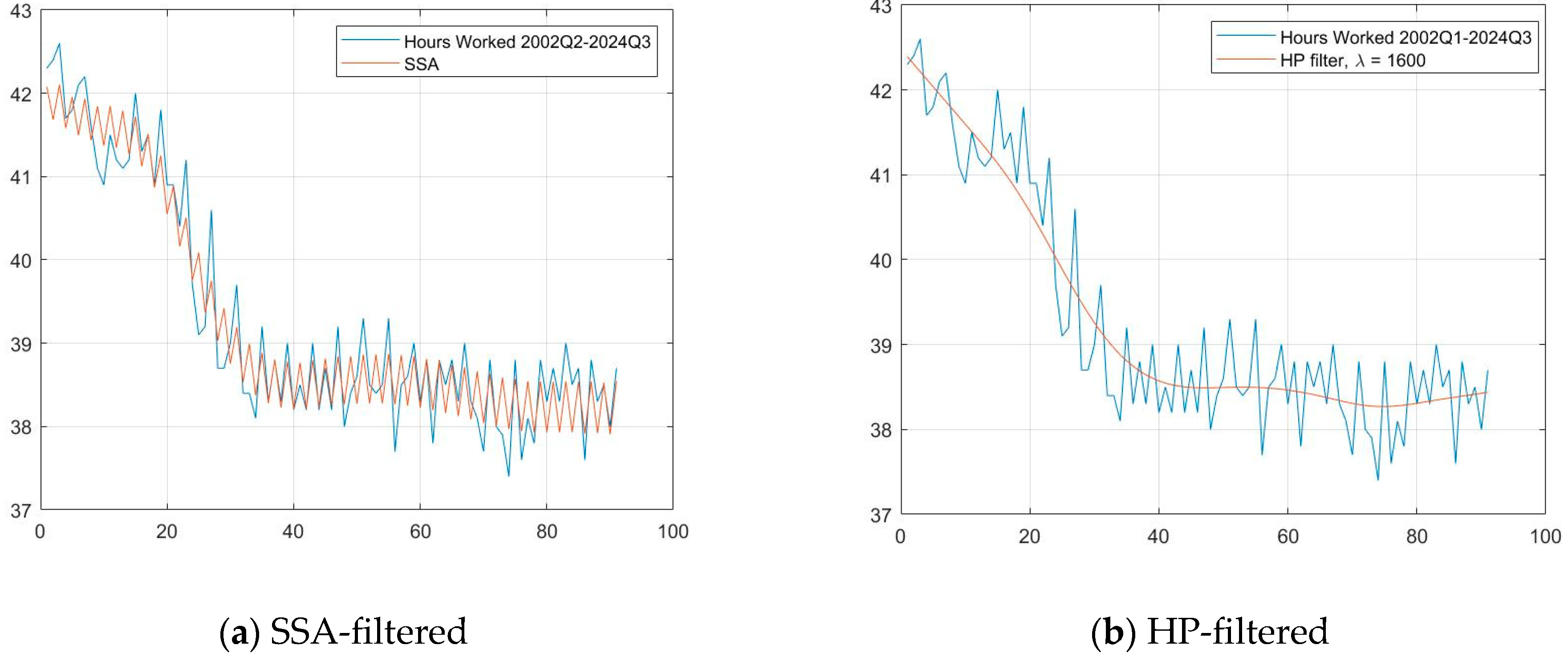
- We used quarterly data for our analysis, 2002Q1–2024Q3. This data interval is based on the availability of labour data, the time series of which starts from 2002Q1.
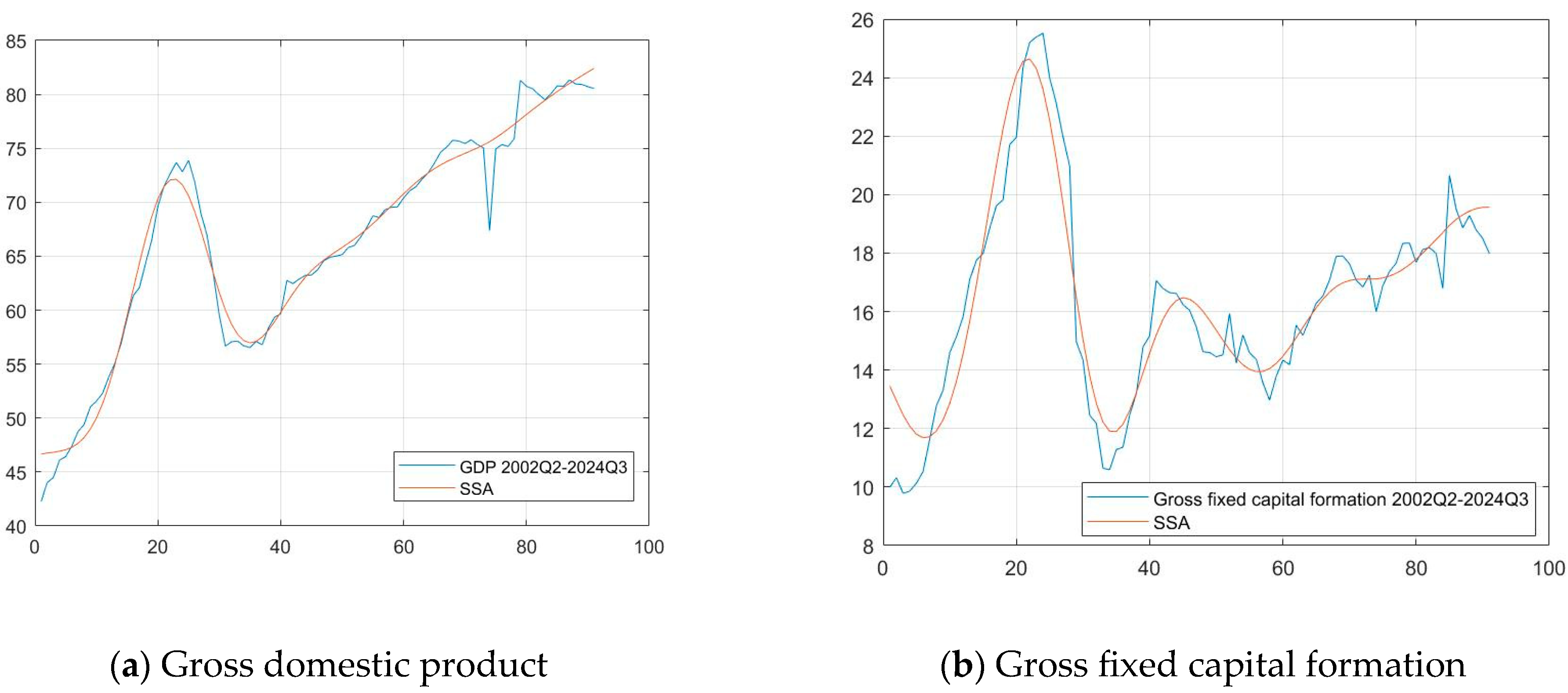
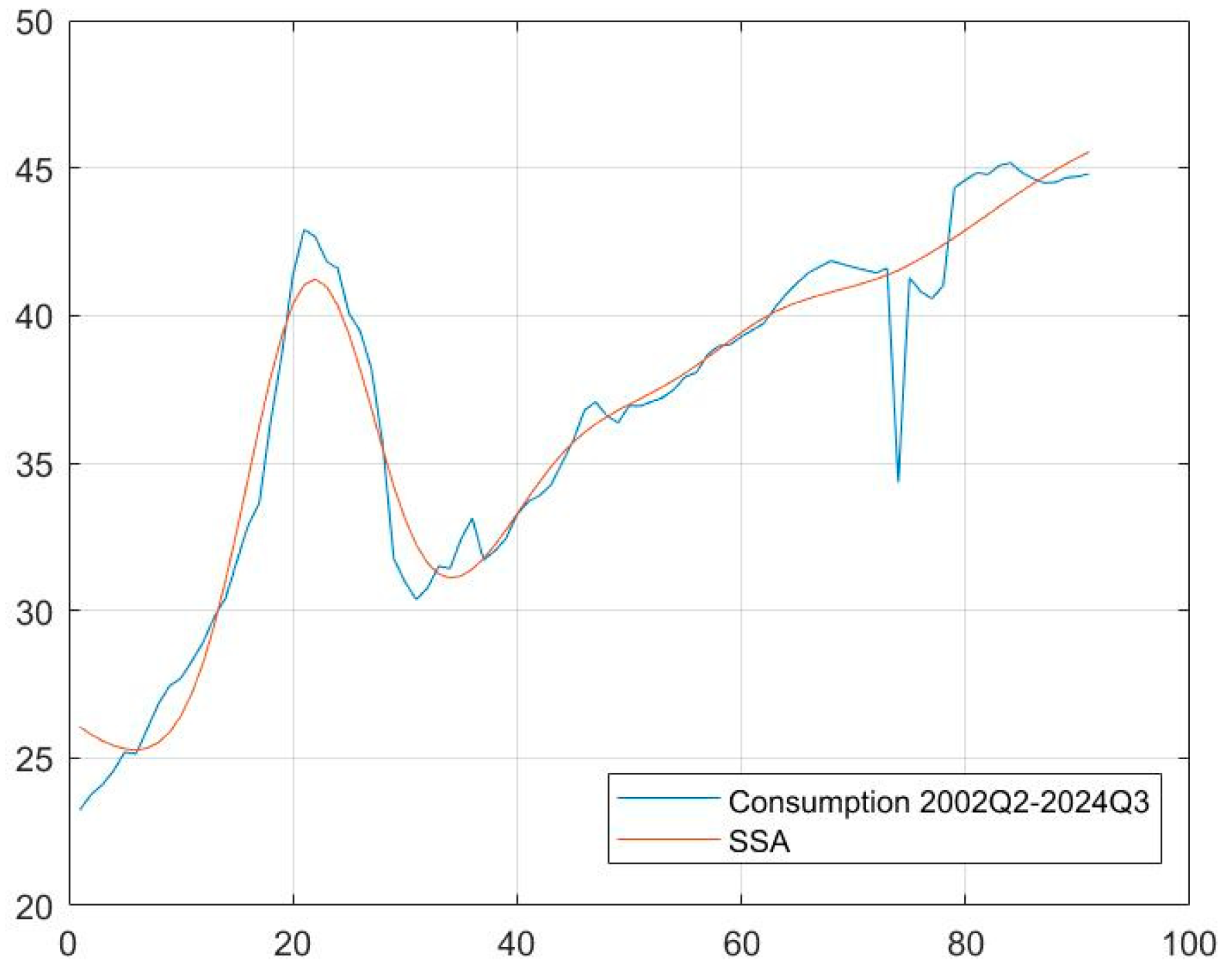
- These four indicators were selected for comparison with Dynare results because they are characterised as the main components of the output (see Equation (6)) and the utility of the household (see Equation (1)). Furthermore, these indicators obtained a strong correlation with the output according to the Dynare results obtained (see Section 5.1).
5. Results
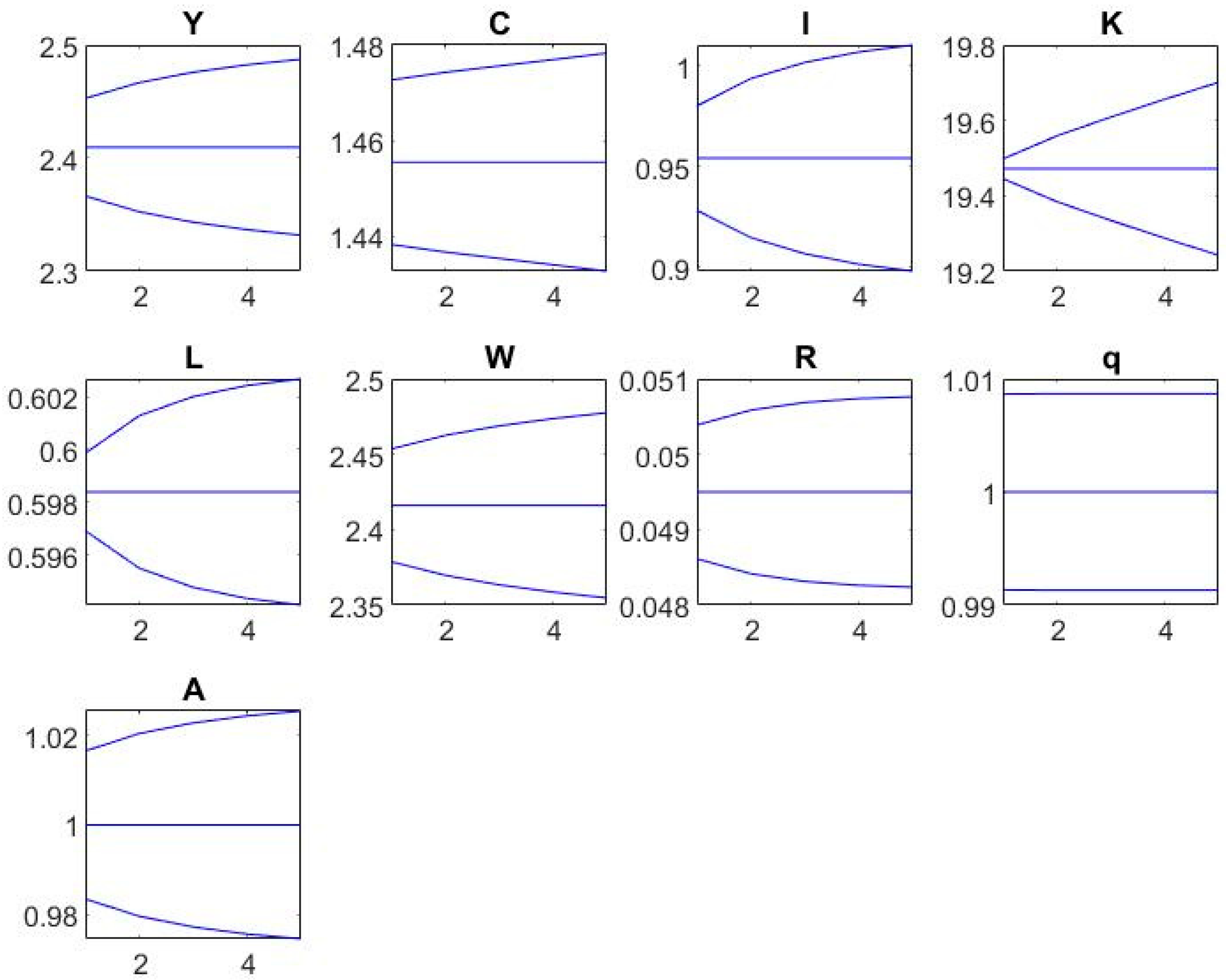
5.1. Dynare Results
- Solution of the steady state of the model. In general, the steady state describes the behaviour of endogenous variables in the long run. The steady-state values are expressed as log-linear approximations since DSGE models do not have an analytical solution.
- Theoretical moments (mean, standard deviation, and variance) describe the ‘average level’ of endogenous variables and deviations from it.
- Correlation matrix.
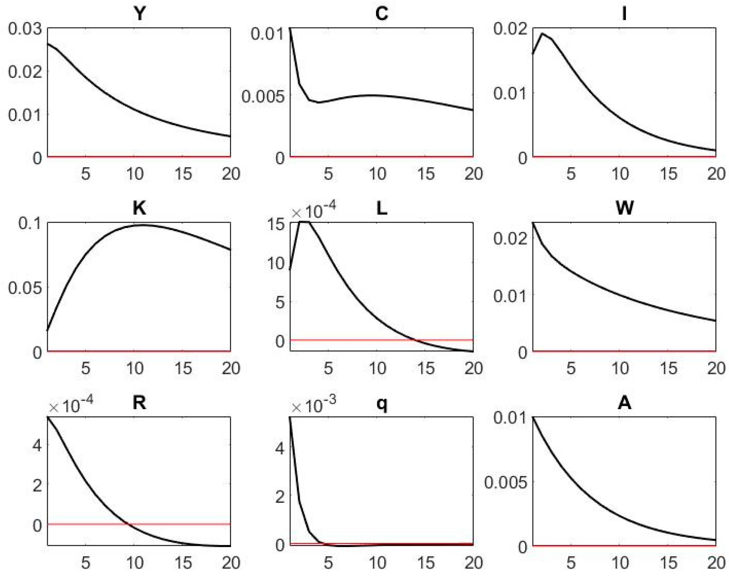
- Impulse response function (IRF) plots.
- Output (‘Y’) and investment (‘I’): 0.9650;
- Output (‘Y’) and wage (‘W’): 0.9904;
- TFP (‘A’) and output (‘Y’): 0.9592;
- TFP (‘A’) and investment (‘I’): 0.9816.
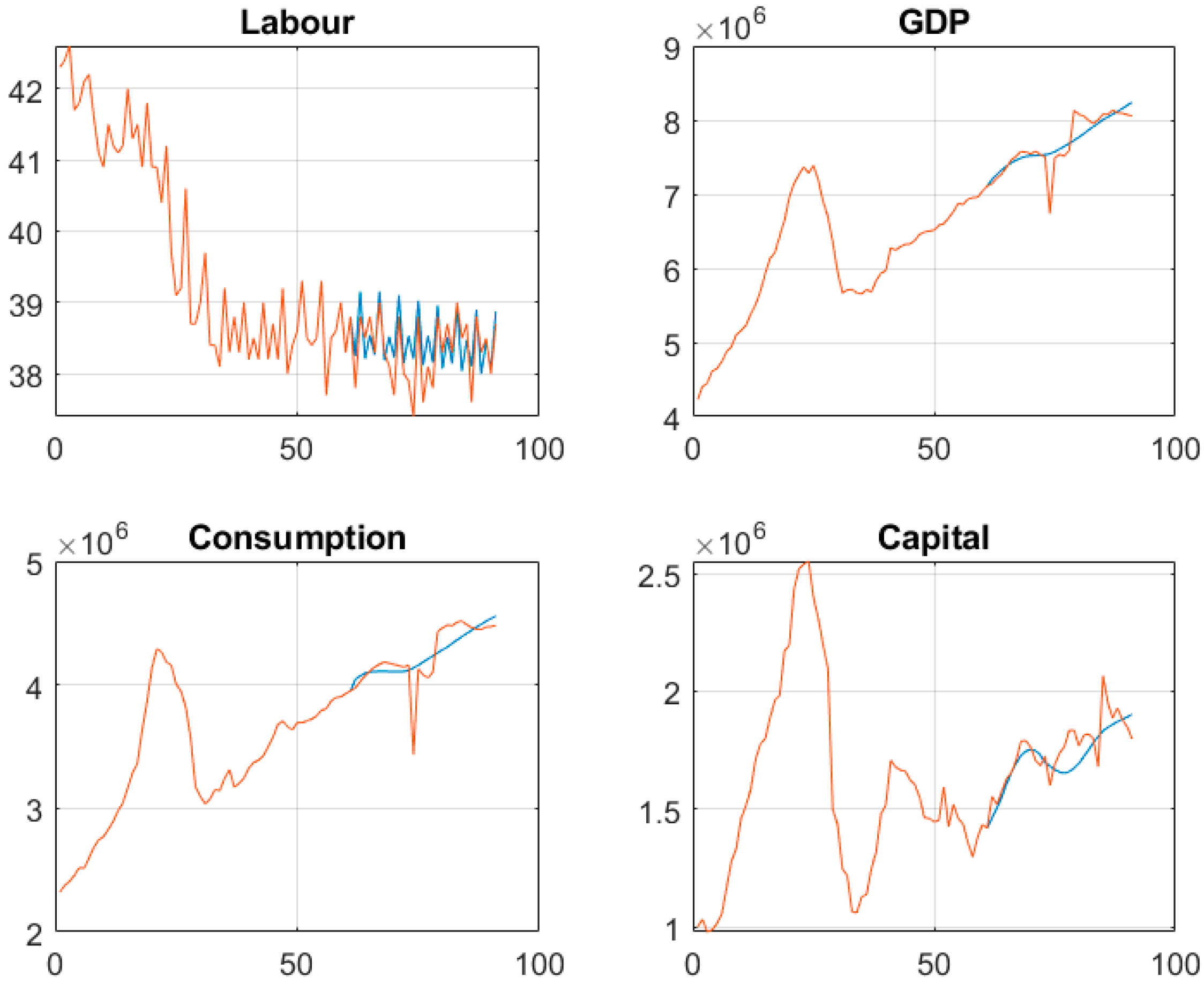
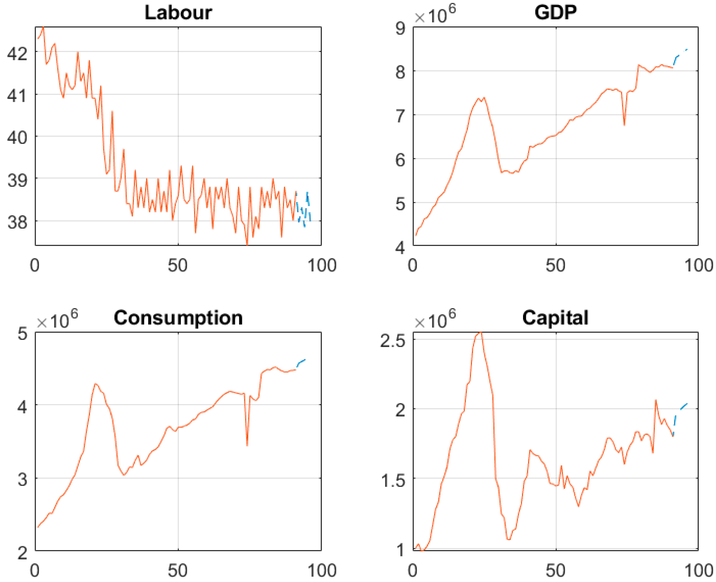
5.2. SSA-Filtered Data Results
5.3. Forecasts
- Labour: 0.74%.
- GDP: 1.46%.
- Consumption: 2.35%.
- Capital: 3.56%.
6. Discussion
7. Conclusions
Author Contributions
Funding
Institutional Review Board Statement
Informed Consent Statement
Data Availability Statement
Conflicts of Interest
Abbreviations
| CV | Coefficient of variation |
| DSGE | Dynamic Stochastic General Equilibrium |
| EU | European Union |
| Eq | Equation |
| FA | Fundamental Analysis |
| HP filter | Hodrick–Prescott filter |
| IRF | Impulse Response Function |
| GDP | Gross Domestic Product |
| KLT | Karhunen–Loeve transform |
| LV | Latvia |
| Log | Logarithmic |
| MAPE | Mean Absolute Percentage Error |
| NK | New Keynesian |
| Q | Quarter |
| RBC | Real Business Cycle |
| RE | Rational Expectations |
| thsd. | Thousand |
| TA | Technical Analysis |
| TFP | Total Factor Productivity |
| STDEV | Standard Deviation |
| SSA | Singular Spectrum Analysis |
| VAR | Variance |
References
- Adjemian. (2018). Understanding forecast methodology in Dynare. General DSGE modeling. Available online: https://forum.dynare.org/t/understanding-forecast-methodology-in-dynare/12566 (accessed on 10 January 2025).
- Becker, C., & Noone, C. (2008). Volatility and persistence of capital flows. Bank for International Settlements Press & Communications. [Google Scholar]
- Birol, Ö. H. (2015). What it means to be a new classical economist. Procedia–Social and Behavioral Sciences, 195, 574–579. [Google Scholar] [CrossRef]
- Bitāns, M., & Purviņš, V. (2012). The development of Latvia’s economy (1990–2004) (pp. 141–147). The Bank of Latvia XC. [Google Scholar]
- Bógalo, J., Poncela, P., & Senra, E. (2024). Understanding fluctuations through multivariate circulant singular spectrum analysis. Expert Systems with Applications, 251, 123827. [Google Scholar]
- Buss, G. (2017). Wage formation, unemployment and business cycle in Latvia (No. 2017/01). Latvijas Banka. [Google Scholar]
- Bušs, G., & Grüning, P. (2023). Fiscal DSGE model for Latvia. Baltic Journal of Economics, 23(1), 1–44. [Google Scholar] [CrossRef]
- Calvo, G. A. (1983). Staggered prices in a utility-maximizing framework. Journal of Monetary Economics, 12(3), 383–398. [Google Scholar] [CrossRef]
- Cherrier, B., Saïdi, A., & Sergi, F. (2023). Write your model almost as you would on paper and dynare will take care of the rest! SSRN Scholarly Paper. [CrossRef]
- Christiano, L. J., Eichenbaum, M. S., & Trabandt, M. (2018). On DSGE models. Journal of Economic Perspectives, 32(3), 113–140. [Google Scholar] [CrossRef]
- Coussin, M. (2022). Singular spectrum analysis for real-time financial cycles measurement. Journal of International Money and Finance, 120, 102532. [Google Scholar] [CrossRef]
- CSB. (2008). Quarterly national accounts inventory. Sources and Methods of Latvia. Central Statistical Bureau of Latvia. [Google Scholar]
- CSB. (2020). Historical facts in short. Central statistical bureau Republic of Latvia. Available online: https://www.csp.gov.lv/en/historical-facts-short (accessed on 20 March 2025).
- De Vroey, M. (2016). A history of macroeconomics from Keynes to Lucas and beyond. Cambridge University Press. [Google Scholar]
- Del Negro, M., & Schorfheide, F. (2013). DSGE model-based forecasting. In Handbook of economic forecasting (Vol. 2, pp. 57–140). Elsevier. [Google Scholar]
- Dynare. (2017). Dynare manual. Available online: https://archives.dynare.org/manual/index_32.html (accessed on 10 January 2025).
- EM. (2008). The national economy of Latvia: A macroeconomic review. Ministry of Economics Republic of Latvia.
- EM. (2024). Macroeconomic review of Latvia. Ministry of Economics Republic of Latvia. Available online: https://www.em.gov.lv/en/media/20010/download?attachment (accessed on 10 January 2025).
- Fernández-Villaverde, J., & Guerrón-Quintana, P. A. (2021). Estimating DSGE models: Recent advances and future challenges. Annual Review of Economics, 13(1), 229–252. [Google Scholar] [CrossRef]
- Ferroni, F., Fisher, J. D. M., & Melosi, L. (2024). Unusual shocks in our usual models. Journal of Monetary Economics, 147, 103598. [Google Scholar] [CrossRef]
- Ferroni, F., Grassi, S., & León-Ledesma, M. A. (2015). Fundamental shock selection in DSGE models. School of Economics Discussion Papers. [Google Scholar]
- Flotho, S. (2009). DSGE models–Solution strategies. Available online: https://www.macro.uni-freiburg.de/publications/data/research_flotho/dsge_models (accessed on 10 January 2025).
- Gastpar, M., Dragotti, P. L., & Vetterli, M. (2006). The distributed Karhunen–Loève transform. IEEE Transactions on Information Theory, 52(12), 5177–5196. [Google Scholar] [CrossRef]
- Golyandina, N. (2020). Particularities and commonalities of singular spectrum analysis as a method of time series analysis and signal processing. Wiley Interdisciplinary Reviews: Computational Statistics, 12(4), e1487. [Google Scholar]
- Golyandina, N., Nekrutkin, V., & Zhigljavsky, A. A. (2001). Analysis of time series structure: SSA and related techniques. CRC Press. [Google Scholar]
- Gomme, P., & Lkhagvasuren, D. (2013). Calibration and simulation of DSGE models. In Handbook of research methods and applications in empirical macroeconomics. Edward Elgar Publishing. [Google Scholar]
- Gu, J., Hung, K., Ling, B. W. K., Chow, D. H. K., Zhou, Y., Fu, Y., & Pun, S. H. (2024). Generalized singular spectrum analysis for the decomposition and analysis of non-stationary signals. Journal of the Franklin Institute, 361(6), 106696. [Google Scholar]
- Herbst, E. (2024). Forecasting with DSGE models. In Handbook of research methods and applications in macroeconomic forecasting (pp. 126–155). Edward Elgar Publishing. [Google Scholar]
- Hinkle, D. E., Wiersma, W., & Jurs, S. G. (2003). Applied statistics for the behavioral sciences. Houghton Mifflin. [Google Scholar]
- IMF. (2025). World economic outlook. Available online: https://www.imf.org/en/Publications/WEO (accessed on 20 March 2025).
- Iskrev, N. (2018). Calibration and the estimation of macroeconomic models. Banco de Portugal Economics and Research Department. [Google Scholar]
- Junior, C. J. C. (2016). Understanding DSGE models: Theory and applications. Vernon Press. [Google Scholar]
- Kehrig, M., Schneider, M., & Cosmin, I. (2014). What drives micro and macro volatility? VoxEU Column (Blog). [Google Scholar]
- Kydland, F. E., & Prescott, E. C. (1982). Time to build and aggregate fluctuations. Econometrica, 50(6), 1345–1370. [Google Scholar] [CrossRef]
- Long, J. B., & Plosser, C. I. (1983). Real business cycles. Journal of Political Economy, 91(1), 39–69. [Google Scholar]
- Lucas, R. E., Jr. (1976). Econometric policy evaluation: A critique. In Carnegie-rochester conference series on public policy (Vol. 1, pp. 19–46). North-Holland. [Google Scholar]
- LVPEAK. (2024). Latvijas produktivitātes ziņojums 2023. Available online: https://www.lvpeak.lu.lv/fileadmin/user_upload/lu_portal/lvpeak.lu.lv/LU_domnica_LV_PEAK/Latvijas_produktivitates_zinojums_2020/2023/2023_LPZ.pdf (accessed on 12 February 2025).
- Navarro, M. M., Young, M. N., Prasetyo, Y. T., & Taylar, J. V. (2023). Stock market optimization amidst the COVID-19 pandemic: Technical analysis, K-means algorithm, and mean-variance model (TAKMV) approach. Heliyon, 9(7), e17577. [Google Scholar] [CrossRef]
- OECD. (2024). OECD economic surveys: Latvia 2024. OECD Publishing. [Google Scholar] [CrossRef]
- Official Statistics Portal. (2025a). Gross domestic product from the expenditure approach (thousand euro). Available online: https://stat.gov.lv/en/statistics-themes/economy/gross-domestic-product-quarterly-data/tables/isp050c-gross-domestic (accessed on 13 January 2025).
- Official Statistics Portal. (2025b). Hours worked on average per week by professional status, sex. Available online: https://stat.gov.lv/en/statistics-themes/labour-market/employment/tables/nbl130c-hours-worked-average-week-professional (accessed on 13 January 2025).
- Ozolin̦a, V., & Pochs, R. (2013). Macroeconomic modelling and elaboration of the macro-econometric model for the Latvian economy: Scientific monograph. Riga Technical University. [Google Scholar]
- Polukoshko, S., Hilkevica, G., & Gonca, V. (2014). Non-stationary vibration studying based on singular spectrum analysis. Vibroengineering Procedia, 3, 133–138. [Google Scholar]
- Polukoshko, S., & Hofmanis, J. (2009). Use of ‘caterpillar’–SSA method for analysis and forecasting of industrial and economic indicators. Environment Technologies Resources. Proceedings of the International Scientific and Practical Conference, 2, 241–248. [Google Scholar] [CrossRef]
- Slanicay, M. (2014). Some notes on historical, theoretical, and empirical background of DSGE models. Review of Economic Perspectives, 14(2), 145–164. [Google Scholar] [CrossRef]
- Thornton, M. A. (2005, May 19–21). The Karhunen-Loeve transform of discrete MVL functions. 35th International Symposium on Multiple-Valued Logic (ISMVL’05) (pp. 194–199), Calgary, BC, Canada. [Google Scholar]
- Torres, J. L. (2016). Introduction to dynamic macroeconomic general equilibrium models. Vernon Press. [Google Scholar]
- Trading Economics. (2025a). Latvia consumer spending. Available online: https://tradingeconomics.com/latvia/consumer-spending (accessed on 12 February 2025).
- Trading Economics. (2025b). Latvia GDP constant prices. Available online: https://tradingeconomics.com/latvia/gdp-constant-prices (accessed on 12 February 2025).
- Trading Economics. (2025c). Latvia gross fixed capital formation. Available online: https://tradingeconomics.com/latvia/gross-fixed-capital-formation (accessed on 12 February 2025).
- Valadkhani, A. (2004). History of macroeconometric modelling: Lessons from past experience. Journal of Policy Modeling, 26(2), 265–281. [Google Scholar] [CrossRef]
- Villemot, S. (2023). Dynare: Macroeconomic modelling for all. Presented at the mathworks finance conference 2023. Available online: https://www.mathworks.com/content/dam/mathworks/mathworks-dot-com/company/events/conferences/mathworks-finance-conference/2023/dynare-macroeconomic-modeling-for-all.pdf (accessed on 10 January 2025).
- Yagihashi, T. (2020). DSGE models used by policymakers: A survey. Policy Research Institute, Ministry of Finance. [Google Scholar]
- Yun, T. (1996). Nominal price rigidity, money supply endogeneity, and business cycles. Journal of Monetary Economics, 37(2), 345–370. [Google Scholar] [CrossRef]
- Zhigljavsky, A. A. (2010). Singular spectrum analysis for time series: Introduction to this special issue. Statistics and Its Interface, 3(3), 255–258. [Google Scholar]

| Parameter | Notation | Value | Source |
|---|---|---|---|
| Capital elasticity | 0.40 | (Bušs & Grüning, 2023) | |
| Discount factor | 0.9995 | (Bušs & Grüning, 2023) | |
| Depreciation rate | 0.0490 | (Bušs & Grüning, 2023) | |
| Consumption preference | 0.60 | (EM, 2024) | |
| Investment adjustment cost | 0.40 | (Bušs & Grüning, 2023) | |
| TFP autoregressive parameter | 0.85 | (Bušs & Grüning, 2023) | |
| TFP standard deviation | 0.01 | (Junior, 2016) |
| Variable in the Model | Empirical Data | Measurement | Data Period | Source |
|---|---|---|---|---|
| Y (output) | Gross domestic product | thsd. euro, in 2020 prices, seasonally adjusted data | 2002Q1–2024Q3 | (Official Statistics Portal, 2025a) |
| C (consumption) | Household final consumption expenditure | thsd. euro, in 2020 prices, seasonally adjusted data | 2002Q1–2024Q3 | (Official Statistics Portal, 2025a) |
| K (capital) | Gross fixed capital formation | thsd. euro, in 2020 prices, seasonally adjusted data | 2002Q1–2024Q3 | (Official Statistics Portal, 2025a) |
| L (labour) | Hours worked on average per week | Hours worked (total, employees) | 2002Q1–2024Q3 | (Official Statistics Portal, 2025b) |
| Variable | Steady-State | Mean | STEV | VAR | Volatility | CV |
|---|---|---|---|---|---|---|
| ‘Y’ | 2.4096 | 2.4096 | 0.0649 | 0.0042 | 1.00 | 2.69% |
| ‘C’ | 1.4555 | 1.4555 | 0.0257 | 0.0007 | 0.40 | 1.77% |
| ‘I’ | 0.9541 | 0.9541 | 0.0434 | 0.0019 | 0.67 | 4.55% |
| ‘K’ | 19.4717 | 19.4717 | 0.4467 | 0.1995 | 6.88 | 2.29% |
| ‘L’ | 0.5984 | 0.5984 | 0.0033 | 0 | 0.05 | 0.55% |
| ‘W’ | 2.4161 | 2.4161 | 0.0548 | 0.003 | 0.84 | 2.27% |
| ‘R’ | 0.0495 | 0.0495 | 0.001 | 0 | 0.02 | 2.02% |
| ‘q’ | 1.0000 | 1.0000 | 0.0056 | 0 | 0.09 | 0.56% |
| ‘A’ | 1.0000 | 1.0000 | 0.019 | 0.0004 | 0.29 | 1.90% |
| ‘Y’ | ‘C’ | ‘I’ | ‘K’ | ‘L’ | ‘W’ | ‘R’ | ‘q’ | ‘A’ | |
|---|---|---|---|---|---|---|---|---|---|
| ‘Y’ | 1 | - | - | - | - | - | - | - | - |
| ‘C’ | 0.8966 | 1 | - | - | - | - | - | - | - |
| ‘I’ | 0.9650 | 0.7491 | 1 | - | - | - | - | - | - |
| ‘K’ | 0.7205 | 0.9070 | 0.5407 | 1 | - | - | - | - | - |
| ‘L’ | 0.8179 | 0.4785 | 0.9401 | 0.2501 | 1 | - | - | - | - |
| ‘W’ | 0.9904 | 0.9492 | 0.9195 | 0.7951 | 0.7304 | 1 | - | - | - |
| ‘R’ | 0.5650 | 0.1924 | 0.7312 | −0.1651 | 0.8702 | 0.4614 | 1 | - | - |
| ‘q’ | 0.5076 | 0.4437 | 0.4966 | 0.0359 | 0.4300 | 0.4991 | 0.6680 | 1 | - |
| ‘A’ | 0.9592 | 0.7655 | 0.9816 | 0.4974 | 0.9073 | 0.9204 | 0.7715 | 0.6523 | 1 |
| Variable | Notation | Calibrated Model (Dynare) | Log-Data (SSA) | ||||
|---|---|---|---|---|---|---|---|
| Mean | STDEV | VAR | Mean | STDEV | VAR | ||
| GDP | Y | 2.4096 | 0.0649 | 0.0042 | −0.0119 | 0.1583 | 0.0251 |
| Consumption | C | 1.4555 | 0.0257 | 0.0007 | 0.5813 | 0.1583 | 0.0251 |
| Capital | K | 19.4717 | 0.4467 | 0.1995 | 1.3846 | 0.1583 | 0.0251 |
| Labour | L | 0.5984 | 0.0033 | 0 | −0.0006 | 0.0336 | 0.0011 |
| Correlation Coefficients | Correlation Strength | |||
|---|---|---|---|---|
| Variables | Dynare | Log-Data SSA | Empirical Data | |
| Y and L | 0.8179 | −0.7074 | −0.64085 | Dynare: high negative Log-data: high negative Empirical data: moderate negative |
| Y and C | 0.8966 | 1 | 0.986729 | Dynare: very high Log-data: absolute Empirical data: very high |
| C and L | 0.4785 | −0.7074 | −0.60826 | Dynare: low positive Log-data: high negative Empirical data: moderate negative |
| K and L | 0.2501 | −0.7074 | −0.07629 | Dynare: low positive Log-data: high negative Empirical data: negligible |
| K and C | 0.9070 | 1 | 0.656115 | Dynare: very high positive Log-data: absolute Empirical data: moderate |
| K and Y | 0.7205 | 1 | 0.643251 | Dynare: high positive Log-data: absolute Empirical data: moderate |
| Indicator | Official Statistics Portal | SSA Forecast | Absolute Percentage Error |
|---|---|---|---|
| 2024Q4 | 2024Q4 | ||
| Gross domestic product | 8,148,036 | 8,287,853 | 1.72% |
| Household final consumption expenditure | 4,483,697 | 4,571,203 | 1.96% |
| Gross fixed capital formation | 1,758,754 | 1,962,917 | 11.61% |
| Hours worked on average per week | 38.3 | 37.96 | 0.89% |
Disclaimer/Publisher’s Note: The statements, opinions and data contained in all publications are solely those of the individual author(s) and contributor(s) and not of MDPI and/or the editor(s). MDPI and/or the editor(s) disclaim responsibility for any injury to people or property resulting from any ideas, methods, instructions or products referred to in the content. |
© 2025 by the authors. Licensee MDPI, Basel, Switzerland. This article is an open access article distributed under the terms and conditions of the Creative Commons Attribution (CC BY) license (https://creativecommons.org/licenses/by/4.0/).
Share and Cite
Hilkevics, S.; Semakina, V. A Comparative Analysis of the Calibrated DSGE Model and SSA Method Results on the Latvian Economy. Economies 2025, 13, 94. https://doi.org/10.3390/economies13040094
Hilkevics S, Semakina V. A Comparative Analysis of the Calibrated DSGE Model and SSA Method Results on the Latvian Economy. Economies. 2025; 13(4):94. https://doi.org/10.3390/economies13040094
Chicago/Turabian StyleHilkevics, Sergejs, and Valentina Semakina. 2025. "A Comparative Analysis of the Calibrated DSGE Model and SSA Method Results on the Latvian Economy" Economies 13, no. 4: 94. https://doi.org/10.3390/economies13040094
APA StyleHilkevics, S., & Semakina, V. (2025). A Comparative Analysis of the Calibrated DSGE Model and SSA Method Results on the Latvian Economy. Economies, 13(4), 94. https://doi.org/10.3390/economies13040094