Modeling Semiarid River–Aquifer Systems with Bayesian Networks and Artificial Neural Networks

Abstract

In semiarid areas, precipitations usually appear in the form of big and brief floods, which affect the aquifer through water infiltration, causing groundwater temperature changes. These changes may have an impact on the physical, chemical and biological processes of the aquifer and, thus, modeling the groundwater temperature variations associated with stormy precipitation episodes is essential, especially since this kind of precipitation is becoming increasingly frequent in semiarid regions. In this paper, we compare the predictive performance of two popular tools in statistics and machine learning, namely Bayesian networks (BNs) and artificial neural networks (ANNs), in modeling groundwater temperature variation associated with precipitation events. More specifically, we trained a total of 2145 ANNs with different node configurations, from one to five layers. On the other hand, we trained three different BNs using different structure learning algorithms. We conclude that, while both tools are equivalent in terms of accuracy for predicting groundwater temperature drops, the computational cost associated with the estimation of Bayesian networks is significantly lower, and the resulting BN models are more versatile and allow a more detailed analysis.

1. Introduction

Rivers of small basins have a limited thermal capacity and are very sensitive to transient thermal disturbances [1], especially those originated from storm episodes. In semiarid areas, precipitations are characterized by a high space-time variability with strong stormy events [2], which affect the aquifer through water infiltration [3], causing groundwater temperature changes [4,5,6]. Groundwater temperature variations have an impact on physical, chemical, and biological processes, including solubility of gases in groundwater, geochemical reaction rates, microbial respiration rates or pathogen propagation [7,8,9]. Since groundwater is a common source of drinking water and irrigation supply, especially in semiarid areas, the identification of the type of precipitation is essential for the proper management of these water bodies, and becomes crucial regarding the fact that the extension of semiarid areas is likely to increase in the future [10].

Groundwater temperature is also a matter of study in other disciplines. For instance, from the renewable energy viewpoint, there is an increasing interest in groundwater temperature due to its potential use as heat pump systems [11,12]. Since the temperature of groundwater is relatively constant, it can be used as a source of geothermal energy for heating in winter and cooling in summer. Moreover, heat is a natural tracer broadly used to typify and quantify surface water–groundwater exchange due to its easiness at measuring [6,13,14,15,16,17,18]. Many works started using water temperature measurements to assess the vertical flows [15,19,20,21] combined with hydraulic data [22,23,24], hydrochemical [25,26], and isotopic [27,28] to get a better interpretation. Therefore, the prediction of groundwater temperature is of widespread interest.

Modeling and predicting the groundwater behavior is a complex task due to its nonlinear nature and the high number of factors involved. This task has been addressed using a wide variety of approaches in the last decades, such as time series, stochastic methods [29], Markov chain Monte Carlo methods [30] or, more recently, machine learning methods, including support vector machines, artificial neural networks or Bayesian networks.

Artificial neural networks (ANNs) have been widely used in hydrology-related areas. An exhaustive review about the applications of ANNs in hydrology can be found in [31] and [32]. The potential of ANNs in forecasting the groundwater level fluctuation has been shown in many studies: Ref. [33] show the superior performance of ANN in groundwater level predictions. The authors of [34] compared the performance of seven different ANN configurations in terms of model prediction efficiency using a single well, whereas [35] took into account nearby wells and climatic parameters and [36] used this methodology to predict groundwater levels in individual wells with one month lead. The reviews [37,38] are of special interest; the former summarizes the methods, input data and conclusions from 67 studies using ANNs, Adaptative neuro-fuzzy inference system, genetic programming or support vector machine from groundwater level modeling, while the latter analyzes the advantages and drawbacks of the use of input selection, different divisions of the data into training, testing and validation subsets, structure and architecture of the model as well as procedures of model calibration and performance evaluation criteria of ANNs used in 216 journal papers published between 1999 and 2007.

The efficacy of ANN in predicting groundwater behavior has been proved in different studies: Ref. [39] proposed a Bayesian training method to predict salinity levels in the River Murray, highlighting the importance of introducing the uncertainty in the ANNs; the proposed method was more robust in real-time scenarios allowing the computation of predictions limits as indicators of the quality of the forecasts. The authors of [40] compared the performance of different ANN models using short length records and show the effectiveness of ANN at predicting monthly groundwater level while [34] compared the performance of seven different ANN configurations in terms of model prediction efficiency. The authors of [41] used the gR4J conceptual model to represent initial catchment conditions in Bayesian ANNs in monthly streamflow forecasting, obtaining much more precise forecast distributions. In relation to other methods, ANNs have shown better accuracy than models based on genetic programming [42] in the forecasting of surface air temperature. Moreover, Ref. [43] showed that ANNs outperform traditional quantile regression techniques at predicting regional flood quantiles, whereas [44] proposed support vector machines and adaptive neuro-fuzzy inference system as more accurate approaches than ANN models. However, Ref. [45] found similar accuracy in prediction of river water temperature among step-wise linear regression, random forest, extreme Gradient Boosting, feed-forward neural networks and two types of recurrent neural networks.

On the other hand, Bayesian networks (BN) [46] provide a framework to integrate both quantitative and qualitative data (field data, results, domain expert knowledge, etc.) as well as to deal with the uncertainty inherent in the groundwater system. The authors of [47] showed that BNs can hold the behavior of a numerical groundwater model and evaluate its descriptive and predictive capability. BNs have been used mainly as a support in decision-making processes. In this way, Ref. [48] proposed BNs to support resource managers of the Hydrogeological Unit Eastern Mancha in their decisions and [49] proposed an Object-Oriented Bayesian network to support water resource management decision-making, simulating the impact of possible water management actions on the water system. The authors of [50] assessed the sustainability of social, economic, and environmental values within coastal lakes making use of BNs, Ref. [51] coupled a BN to an evolutionary multi-objective optimization process to analyze a strategy in the negotiations between the Copenhagen Energy and the farmers regarding compensation payment to encourage the reduction of pesticide application in agricultural areas. The authors of [52] developed a Decision Support System based on Dynamic Bayesian Networks for assessing the impacts in an over-exploited aquifer system caused by different Climate Change scenarios. The authors of [53] used BNs to model extreme river discharges in Europe using only geographical properties of catchments; the proposed model was as accurate as other large-scale hydrological models in simulating mean annual maximum of daily discharges being able to create basic flood scenarios at ungauged locations. The authors of [54] improved the capability of BNs for uncertainty estimation by developing a framework for incorporating the uncertainties associated with parameters, input and structures into BNs, and evaluated its relevance in hydrologic forecasting. In addition, Ref. [55] improved the efficiency of the learning of the hierarchical BN by using an incremental data selection algorithm to update the training BN when modeling the flow rate values for small rivers.

In this work, we compare the efficiency of BNs and ANNs in modeling groundwater behaviors. In particular, we are interested in modeling the groundwater temperature variations associated with stormy precipitation episodes. To do so, we have carried out a comparative study, in which all possible configurations of ANNs with one to four layers, as well as a sample of ANNs with 5 layers, have been trained and their predictive performance compared in terms of 6 different metrics. In addition, we have trained and evaluated three different BNs using different structure learning algorithms: naive Bayes, tree augmented network and hill-climbing. The remaining of the paper is organized as follows. Section 2 is devoted to the methodological aspects of the paper. In particular, we describe the study area, data source and data pre-processing in Section 2.1 and Section 2.2; we briefly introduce ANNs and BNs in Section 2.3; and propose scenarios of change in Section 2.4. The performance of the models is analyzed in Section 3, and the results discussed in Section 4. The paper ends with conclusions in Section 5.

2. Material and Methods

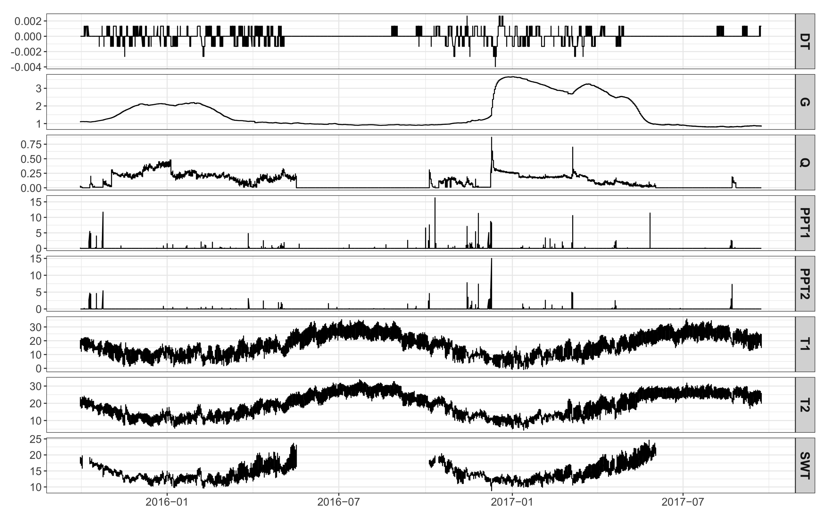
2.1. Study Area and Data Description

The study area (Figure 1) is located in the Andarax river (Southeastern Iberian Peninsula), in a temporal stream reach [56]. This area has some characteristics of a typical semiarid climate, including mild temperatures in the winter and long, dry and warm summers. Precipitation tends to be approximately 200 mm/year [57] and occurs in the form of convective storm systems [58,59], with up to 70% of the annual precipitation taking place over 25% of the rainy days [60]. The hydrology is conditioned by the special rainfall regime, which, as a Mediterranean river, is distinguished by rain and snow and has a swift hydrologic response [61].

The river flows over some Quaternary alluvial deposits (number 5 in Figure 1) that form a small and highly permeable aquifer [62]. A loamy and sandy-loamy formation number 6 in Figure 1 with low permeability [63] is situated on both sides of the alluvial materials [62,64], disconnecting them from the limestone and dolomites (number 8 in Figure 1) that make up the carbonated aquifer system of the Sierra de Gádor range [65]. Downstream is the Plio-Quarternary aquifer, made up of fluvial-deltaic, sandy-loamy conglomerates of continental origin (number 9 in Figure 1) [66] and in connection with the alluvial aquifer.

Since we are interested in modeling the groundwater temperature variations associated with stormy precipitation episodes, the variables considered for the model are those that change over time. Therefore, some other factors that influence groundwater behavior but are constant, such as the geological characteristics of the catchment, were not considered as they should not influence the groundwater temperature variations. The data used in this study were extracted from a control network made up of sampling points of air temperature and precipitation at two meteorological stations; surface water temperature and flow level at the gauging station; and groundwater temperature and piezometric level (Figure 1,

Table 1. Description of variables used in the models of this study. Data were measured hourly.

Variables	Abbreviation
Groundwater temperature, measured as the difference of two consecutive time steps	DT
Groundwater table	G
Flow volume	Q
Precipitation at Station 1	PPT1
Precipitation at Station 2	PPT2
Air temperature at Station 1	T1
Air temperature at Station 2	T2
Surface water temperature	SWT

). All the measurements were obtained at hourly intervals from October 2015 to September 2017 (Figure 2). Precipitation and water flow level data come from two meteorological stations and one gauging station of the Ministry of the Environment and Territorial Planning of the Regional Government of Andalusia, situated in the subsystem IV of the province of Almeria-River basin of the Andalusian Mediterranean Watersheds (Figure 1). For the piezometric level and temperature data, HOBO U20-001-02 pressure and temperature data loggers were used: two for air temperature, one in the river for surface water temperature, and another to measure the groundwater temperature (8 meters) (Figure 1). The place where the groundwater data logger is installed is situated over the alluvial at a short distance from the surface water. Air and water temperature was measured in °C, groundwater and flow level in meters, and precipitation in mm.

2.2. Data Pre-Processing

Raw groundwater temperature data were used to compute the groundwater temperature change ($DT$), which represents the difference in temperature between two consecutive time steps. More precisely, given two consecutive time steps, t and $t+1$, $DT=T_{t+1}-T_t$, where $T_{t+1}$ is the groundwater temperature at time $t+1$ and $T_t$ is the groundwater temperature at time t.

On the other hand, the remaining raw data measures were shifted based on the observed lag between the response variable (groundwater temperature change) and each predictive variable. The lags represent the delay between a change in a variable and its corresponding response in the groundwater temperature. In order to do that, the cross-correlation between the response and the predictive variables was computed.

Table 2. Observed lag (in hours) between the groundwater temperature and the predictive variables.

Predictive Variable	Lag (in Hours)
Groundwater table (G)	0
Flow volume (Q)	48
Precipitation at Station 1 (PPT1)	72
Precipitation at Station 2 (PPT2)	70
Air temperature at Station 1 (T1)	5
Air temperature at Station 2 (T2)	5
Surface water temperature (SWT)	5

shows the observed lag, used to shift the time series.

After shifting the time series, the initial 17,352 observations were filtered to keep only those in which precipitations events occurred. This process removed nearly 98% of the instances, yielding a dataset of 383 observations.

Next, an exploratory analysis was carried out to find redundant variables. Since severe collinearity was found between variables T1 and T2 (with variance inflation factors equal to 14.31 and 15.43, respectively, correlation coefficient equal to 0.9626 and a p-value under 0.001 in the Bartlett’s test of sphericity), a Principal Component Analysis was performed to obtain a new variable (T) that picks up the information of T1 and T2. To sum up, the data pre-processing yielded a dataset of 383 observations taking values over 7 variables. Figure 3 shows the histograms of the six predictive variables used to model the response variable (DT).

Finally, since our goal is to determine when the temperature in the aquifer decreases ($DT<0$), the variable DT was discretized into two classes (D = ‘temperature drop’ and N = ‘no temperature drop’), with 100 and 283 observations in each class, respectively. We have used the raw (continuous) predictive variables to train the ANNs. On the other hand, given that the software we have used for estimating the BNs only handles discrete or Gaussian variables, and the predictive variables involved in this study are not Gaussian, we have discretized them into equal frequency interval classes by the function $equal\_freq$ from the R package funModelling [67]. We have tried to split the variables in as many classes as possible, taking 40 interval classes for variables G, SWT and T and 16, 22 and 27 for PPT1, PPT2, and Q, respectively, since the high skewness of these variables causes many empty interval classes when they are split in more intervals.

2.3. Artificial Neural Networks and Bayesian Networks

An artificial neural network (ANN) is a structure formed of several layers with nodes arranged in each one. The first layer, called input layer, consists of the input variables for the problem. The last layer, called output layer, consists of the values predicted by the ANN, constituting the model output. Between the input and output layers, there are one or more hidden layers whose nodes are fully connected to those in the previous and next layers but not to those in the same layer. Figure 4 shows an example of an ANN with one hidden layer and three nodes in it.

The connection link between nodes i and j has an associated weight, $W_{ij}$, which represents the connection strength between both nodes. Besides, each node has associated a threshold or bias that must be exceeded in order to activate it. If a node is activated, its output is computed as the value of a so-called activation function, with respect to the product of the vector of inputs and weights associated with the node, minus the threshold. The role of the activation function can range from simply activating the node to transforming input signals to output signals.

Once the number of layers and nodes in each layer is fixed, as well as the activation function to be used, the training process, or learning, consists of finding the optimal weights and thresholds which minimize the error in the ANN output. The activation function can be chosen from a wide range of functions (the most commonly used are the logistic, hyperbolic tangent, ReLu, and Softmax functions) and the training process from a set of learning algorithms available in the literature. However, the hardest task when deciding the architecture of the ANN is to decide the number of hidden layers and the number of nodes in each layer because there is no procedure to determine both attributes and, thus, they are usually determined ad hoc. The chosen number of hidden layers can affect significantly the performance of the ANN: too few nodes may lead to poor approximations whereas too many nodes are likely to overfit the training data.

Bayesian networks (BN) offer an alternative procedure to avoid this issue. A BN [46,68] is a statistical multivariate probabilistic graphical model described by two components: the structure of the network and the conditional distributions of each node given its parents. The structure of the network consists of a directed acyclic graph (DAG), where each variable is represented by a node and the presence of an edge linking two nodes indicates the existence of statistical dependence between them. Figure 5 shows an example of the structure of a BN with five variables. This structure allows to analyze which variables have an effect on the target variables without the need for numerical calculations since the network structure encodes the conditional independence relations between the variables according to the d-separation criterion [69].

Moreover, the network structure encodes a factorization over the joint distribution of all the variables, which, for the network in Figure 5 is

$$P(x_1,\dots ,x_5)=p\left(x_1\right)·p\left(x_2\right)·p\left(x_3\right|x_1,x_2)\left(x_4\right|x_2)·p\left(x_5\right|x_3).$$

Hence, a BN is fully specified just by giving a conditional distribution for each variable given its parents.

The structure of a BN can be learned by hand (from expert knowledge) or from data, using any structure learning algorithm. See [70] for a thorough review on structure learning algorithms and available software tools. A commonly used score-based algorithm is the Hill-Climbing (HC) search [71], which, briefly speaking, starts from a DAG with no edges and then adds, deletes, and reverses one at a time in order to increase the network score. For BN classifiers, one can also choose fixed or restricted structures, including the Naive Bayes (NB) [72,73] and Tree Augmented Network (TAN) [73] structures. The former is the simplest structure, in which the variable of interest (called the class) is the parent of the remaining predictive variables, which are independent of each other given the class (Figure 6, left). This independence assumption is relaxed in the TAN structure, since it expands the NB structure by allowing each predictive variable to have one more parent besides the class (Figure 6, right). In general, there are several possible TAN structures for a set of variables so, in order to choose among them, a maximum weight spanning tree containing the predictive variables is constructed, using the mutual information between the linked variables, conditioned on the class, as the weight of each edge [73].

To compare the performance of the classifiers based on ANNs and BNs, we have trained the two most commonly used feed-forward back-propagation neural networks: multilayer perceptron (MLP) [74] and radial basis function networks (RBFN) with the dynamic decay adjustment (DDA) algorithm [75]. The activation function used was also the most commonly used in the bibliography for binary classification, this is the logistic (or sigmoid) activation. Although the use of only one hidden layer is more common, to study in depth the classification skill of the ANNs, we have considered all the possible configurations of nodes from one up to four layers and, due to the high computational cost, a random sample of node configurations for ANN with five layers was drawn. In total, 2.145 ANNs were trained and evaluated. The R package RSNNS [76] was used to build the ANNs.

In the case of BN, we have chosen the simplest structure (NB), the tree-augmented network (TAN) structure and the hill-climbing (HC) algorithm for structure learning. The R package bnlearn [77] was used to learn the parameters from data, using the maximum likelihood estimate (MLE) and Bayesian parameter estimation, and to learn the network structure, in the case of TAN and HC. Classification is carried out by the Bayesian networks as a prediction task in which the predicted class c of the target variable DT is computed as the one maximizing the posterior distribution of DT given the observed values of the predictive variables:

$$c=argmaxP\left(c\right|x_1,\dots ,x_n)\mathrm{with} c\in {\mathrm{\Omega }}_{DT}.$$

To evaluate the performance of the different classifiers, the k-fold cross-validation technique [78] was used, with k = 5, and as the accuracy criteria, we have computed the following measures:

• Classification ACCURACY: ratio of the number of correct predictions to the total number of predictions;
• RECALL or sensitivity: true positive rate, computed as

  $$Recall=\frac{TruePositive}{TruePositive+FalseNegative}$$
• PRECISION: ratio of the correctly classified positives to the total classified instances:

  $$Precision=\frac{TruePositive}{TruePositive+FalsePositive}$$
• F-SCORE: balance between precision and recall by computing the harmonic mean;
• G-MEAN: geometric mean of the recall and 1−False Positive rate, which tries to measure the equilibrium between the performance on both, classifying the majority and the minority classes;
• AUC: area under the ROC curve, which measures the ability of the classifier to distinguish between both classes.

2.4. Scenarios of Change

Of special interest is the analysis of different scenarios to study how some changes in the predictive variables influence the behavior of the response variable. The study area shows typical characteristics of a semi-arid climate, with precipitations being around 200 mm/year [57], reaching up to 700 mm/year in the highest peaks. Commonly, precipitations appear as stormy episodes [59], where 70% of the annual precipitation takes place over hardly 25% of the rainy days [60]. This kind of rainfall is usually associated with convective storm phenomena [58]. On the other hand, Mediterranean rivers have a character markedly associated with rainfall and snow, showing an immediate hydrological response [61]. The special precipitation regime directly conditions the hydrological regime in the study area.

Both, ANNs and BNs are able to obtain the predicted class c of the target variable given known values of the regressors. Moreover, BNs are able to return not only the predicted class but also the full probability distribution of a variable of interest thanks to its probabilistic nature, which allows to identify to which extent changes in the regressors have an impact on the response variable. In other words, once we know which variables ($X_E$) have a direct bearing on the target variable ($X_T$), the distribution $p\left(x_T\right|x_E)$ can be used as a measurement of the likelihood of $X_T$ given each possible scenario of $X_E$. This probability distribution can be computed by means of algorithms that make use of the factorization encoded by the network structure [79,80]. There are a number of efficient exact and approximate inference algorithms, such as Variable elimination [81] or Penniless propagation [82], providing a powerful combination of predictive, diagnostic, and explanatory reasoning [83].

Based on the meteorological and hydrological characteristics of the study area, we are interested in the posterior probability distribution of DT when the precipitation events are abundant (i.e., $PPT1\ge 5$ mm/hour or $PPT2\ge 5$ mm/hour) and when they are poor (i.e., $PPT1<1$ mm/hour or $PPT2<1$ mm/hour). To do so, we learnt a new BN, with the predictive variables $PPT1$ and $PPT2$ being discretized into the values Low (L), for values in the interval class $[0,1)$, Moderate (M) for values in the interval class $[1,5)$ and High (H) for values in the interval class $[5,30)$. The hill-climbing algorithm was used to learn the model structure. The R package gRain [84] was used to compute the posterior probability distribution of the response variable.

3. Results

3.1. Predictive Accuracy Comparison between ANNs and BNs

The goal of the built models is to classify the behavior of the groundwater, measured as the difference of temperature ($DT$) and labeled depending on whether the temperature decreases or not, between two consecutive time steps (hours).

Table 3. Performance comparison between ANNs and BNs as classifiers. $HL$: hidden layers. Numbers shown in parentheses in best configuration indicate the number of nodes in each hidden layer.

Network	Best Configuration	ACCURACY	AUC	G-MEAN	PRECISION	RECALL	FSCORE
MLP (1 HL)	5	$0.8628$	$0.8023$	$0.7769$	$0.8503$	$0.7500$	$0.7500$
MLP (2 HL)	(3,4)	$0.9018$	$0.8691$	$0.7711$	$0.8552$	$0.6000$	$0.6667$
MLP (3 HL)	(4,4,4)	$0.9085$	$0.8735$	$0.7650$	$0.7824$	$0.6500$	$0.6842$
MLP (4 HL)	(4,3,1,4)	$0.9086$	$0.8493$	$0.3100$	$0.9167$	$0.5000$	$0.6667$
MLP (5 HL)	No discrimination skill
RBFN with DDA algorithm		$0.8535$	$0.7910$	$0.8068$	$0.7778$	$0.7000$	$0.7368$
Naive Bayes		$0.8824$	$0.8171$	$0.8036$	$0.8945$	$0.9825$	$0.9573$
TAN		$0.6709$	$0.6643$	$0.6587$	$0.8506$	$0.7018$	$0.7767$
HC		$0.8652$	$0.7900$	$0.7663$	$0.8798$	$0.9298$	$0.9217$

displays the average metrics resulting from the cross-validation. In the case of ANN, it is shown the best configuration of nodes for each number of hidden layers. Given a certain number of hidden layers, the best configuration represents the configuration of nodes that yield the highest area under the ROC curve (AUC). This measure has been chosen to summarize the classification performance because it shows the ability of the model at distinguishing between classes.

Among 590 randomly sampled MLP with five hidden layers, none of them could classify properly the positive class (D=Temperature drop) and neither could 50.08% of the MLP with four hidden layers (649 networks). This might be due to the limited sample size available for the classification task. In BNs, the best scores were obtained using the Bayesian parameter estimation for the Naive Bayes structure and the Maximum Likelihood parameter estimation for the HC structure.

Table 3 shows high AUC values, indicating a good level of performance of all the models with exception of the TAN model. MLP with three hidden layers gives the best score in both accuracy and AUC, and BN-based models score higher than RBF in these two metrics. RBF and Naive Bayes classifiers attained the best G-mean. In general, ANN classifiers obtained lower results in RECALL and F-SCORE than BN classifiers, indicating that BN classifiers are more robust than ANN classifiers when a huge amount of data is not available.

An important advantage of BNs is that the computational cost is dramatically reduced, compared with ANNs. Besides, BNs do not require a specification of the number of layers and the configuration of nodes in each layer in advance. This is not an insignificant question because the precision of the classification can vary in an important way. For example, in our dataset, the G-MEAN of the classification given by the MLP with three layers and node configuration $(6,5,5)$ is $0.850109032$, whereas the same MLP, with four layers and node configuration $(2,1,3,2)$ yield a G-MEAN of $0.154010708$; this is more than five times lower than the previous one. The variability between the other metrics can also be important depending on the configuration of the nodes: MLP with configuration $(4,2,5)$ almost doubles the RECALL of the classifier MLP with configuration $(3,6)$ (0.96 and 0.578947368, respectively) and the FSCORE of the MLP with three hidden layers and node configuration $(4,2,5)$ is 52.6% higher than the FSCORE of the MLP with two hidden layers and node configuration $(3,6)$.

Classifiers based on RBF with DDA algorithm do not present this problem but classifiers based on BNs yield higher or similar values in all the performance metrics. Moreover, BNs allow to analyze to which extent changes in the predictive variables have an impact on the response variable thanks to the computation of the conditional probability of the target variable given its parents in the network as we show in the next subsection.

3.2. Evidence Propagation in Bayesian Networks

In this study, the quantitative component of the BNs was used to identify the drops in the temperature of the aquifer (variable $DT$) caused by changes in the precipitation. More specifically, we are interested in obtaining the posterior probability distribution of DT when the precipitation events are abundant, moderate and poor. To do so, we built a new BN, with variables $PPT1$ and $PPT2$ discretized in three intervals, instead of 16 and 22 intervals, respectively, used in the classification problem. We used the hill-climbing algorithm for the structure learning to analyze the relationships obtained between the variables. Figure 7 shows the DAG of the model learned to perform the probabilistic update.

It can be noted that three out of the six predictive variables are not connected in the network structure, which means that they do not have any effect on the target variable. Therefore, only variable $PPT2$ was used as evidence to obtain the posterior probability distribution of $DT$. The other three predictive variables are connected to $DT$ as in the naive Bayes structure. Therefore, they are independent of the other variables given the target variable, $DT$.

Table 4. Performance of the BN used for the propagation task. The measures are the average metrics resulting from the 5-fold cross-validation.

ACCURACY	AUC	G-MEAN	PRECISION	RECALL	FSCORE
0.8809	0.8071	0.7841	0.8871	0.9474	0.931

shows the performance metrics of this classifier. These metrics indicate a good performance of the classifier and are higher than those reported by HC in the comparison of BNs and ANNs (Table 3).

Table 5. Propagation of evidence in $PPT2$. States of variables DT: D: temperature drops; N: temperature does not drop. States of variable $PPT2$: L: low; M: moderate; H: high.

Evidence on PPT2	Posterior Probability Distribution of DT
	D	N
L	0.1737	0.8263
M	0.3192	0.6809
H	0.8333	0.1667

and Figure 8 show the behavior of the groundwater temperature depending on the intensity of the precipitation: light precipitations (<1 mm) hardly cause a change in the temperature, whereas the probability of a drop in the groundwater temperature when the precipitation is moderate (1–5 mm) increases from 26.1% to 32%. When precipitations are greater than 5 mm/h at the meteorological station 2, the probability of a drop in the temperature of the aquifer is 83%.

4. Discussion

The rivers of the small basins have a limited thermal capacity and are very sensitive to transient thermal disturbances [1], revealing a vulnerability in the case of any disruption [85], especially with storm episodes that affect the aquifer through water infiltration [3]. The infiltration and flow of the river are directly associated with the precipitations, but the way in which they take place conditions the infiltration of water in the aquifer [4,5]. The arrival of the water to the aquifer causes temperature changes [6], with the most extreme temperatures being associated with intense water infiltration. It is necessary to understand this behavior, especially in areas of potentially high risk of waste discharge or presence of pollutants, since episodes of quick aquifer recharge may affect the dissolution, precipitation, and mobilization of substances, which could imply a potential risk in terms of groundwater pollution. The proposed methodology might be useful to anticipate these events, and can be applied to other aquifer systems (detritial and carbonate), whose results will depend on their environmental characteristics and particularities.

While the excellent performance of MLP as classifiers is unquestionable, BNs perform better at classifying the positive class (temperature drops), scoring much higher on RECALL (true positive rate) and F-SCORE than ANNs. Therefore, classifiers based on NB or HC structures are both precise and robust in the sense that they do not miss a significant number of instances, saving computational cost and avoiding the decision about the configuration of hidden layers and nodes. Furthermore, BNs offer two advantages to improve the understanding of the problem: the structure of the BN and the probability distribution of the target variable.

The structure of the BN offers a framework of the problem that allows the identification of the variables with an impact on the target variable through the statistical dependency denoted by the edges of the graph. In this sense, the structure of the BN in Figure 7 reveals that precipitations at the meteorological station 1 have no significant effect on the temperature of the groundwater. According to [86], small variations in temperature appear in alluvial groundwater due to precipitations, which become increased after storms. In our case, the use of the structure of the BN highlights the relevance of the distance between the rainfall episode and the aquifer.

On the other hand, the evidence propagation operation allows to determine which variables (or which values of the variables) have a significant impact on the target variable. The propagation analysis in our study shows that precipitation intensities above 5mm/h at the meteorological station 2 cause a large increase in the probability of a drop of temperature, which indicates a fast infiltration of water to the aquifer [87].

5. Conclusions

Bayesian networks constitute an appropriate methodology to reach a better understanding of the system and the relation between storm episodes and the groundwater. The experiments carried out in this paper show that, in general, both ANNs and BNs perform well as classifiers, with BNs showing better performance skills at classifying the positive class. Moreover, BNs show other advantages over ANNs. The computational cost associated with the estimation of BN models is significantly lower, and the resulting model is more versatile. In addition, the BN structure (in the case of HC) is informative about the predictive variables that have an impact on the target variable. Furthermore, BNs facilitate the analysis of different scenarios using the evidence propagation operation, where the likelihood of the outcomes resulting from instantiating the observable variables can be easily computed, which lets us assess to what extent changes in the values of the predictors modify the target variable. These features of the BN might be useful to ensure the proper management of resources.

References

1. Gu, C.; Anderson, W.P., Jr.; Colby, J.D.; Coffey, C.L. Air-stream temperature correlation in forested and urban headwater streams in the Southern Appalachians. Hydrol. Process. 2015, 29, 1110–1118. [Google Scholar] [CrossRef]
2. Thornes, J.B. Catchment and Channel Hydrology. In Geomorphology of Desert Environments; Springer: Berlin/Heidelberg, Germany, 1994; pp. 257–287. [Google Scholar] [CrossRef]
3. Russo, S.L.; Taddia, G.; Dabove, P.; Abdin, E.C.; Manzino, A.M. Effectiveness of time-series analysis for thermal plume propagation assessment in an open-loop groundwater heat pump plant. Environ. Earth Sci. 2018, 77, 1–11. [Google Scholar] [CrossRef]
4. O’Connor, M.T.; Moffett, K.B. Groundwater dynamics and surface water-groundwater interactions in a prograding delta island, louisiana, USA. J. Hydrol. 2015, 524, 15–29. [Google Scholar] [CrossRef]
5. Subyani, A.M. Use of chloride-mass balance and environmental isotopes for evaluation of groundwater recharge in the alluvial aquifer, wadi tharad, western saudi arabia. Environ. Geol. 2004, 46, 741–749. [Google Scholar] [CrossRef]
6. Stonestrom, D.A.; Constantz, J. Heat as a Tool for Studying the Movement of Ground Water near Streams; US Department of the Interior, US Geological Survey: Charleston, SC, USA, 2003; Volume 1260. [Google Scholar]
7. Figura, S.; Livingstone, D.M.; Kipfer, R. Forecasting groundwater temperature with linear regression models using historical data. Groundwater 2015, 53, 943–954. [Google Scholar] [CrossRef]
8. Tissen, C.; Benz, S.A.; Menberg, K.; Bayer, P.; Blum, P. Groundwater temperature anomalies in central Europe. Environ. Res. Lett. 2019, 14, 104012. [Google Scholar] [CrossRef] [Green Version]
9. Agudelo-Vera, C.; Avvedimento, S.; Boxall, J.; Creaco, E.; de Kater, H.; Di Nardo, A.; Djukic, A.; Douterelo, I.; Fish, K.E.; Iglesias Rey, P.L.; et al. Drinking water temperature around the globe: Understanding, policies, challenges and opportunities. Water 2020, 12, 1049. [Google Scholar] [CrossRef] [Green Version]
10. United Nations. Earth Summit: Convention on Desertification. In Proceedings of the ON t.p.: United Nations Conference on Environment and Development, Rio de Janeiro, Brazil, 3–14 June 1992; United Nations: New York, NY, USA, 1994. [Google Scholar]
11. Russo, S.L.; Taddia, G.; Gnavi, L.; Verda, V. Neural network approach to prediction of temperatures around groundwater heat pump systems. Hydrogeol. J. 2014, 22, 205–216. [Google Scholar] [CrossRef]
12. Rock, G.; Kupfersberger, H. 3D modeling of groundwater heat transport in the shallow Westliches Leibnitzer Feld aquifer, Austria. J. Hydrol. 2018, 557, 668–678. [Google Scholar] [CrossRef]
13. Kalbus, E.; Reinstorf, F.; Schirmer, M. Measuring methods for groundwater-surface water interactions: A review. Hydrol. Earth Syst. Sci. 2008, 10, 873–887. [Google Scholar] [CrossRef] [Green Version]
14. Anibas, C.; Fleckenstein, J.H.; Volze, N.; Buis, K.; Verhoeven, R.; Meire, P.; Batelaan, O. Transient or steady-state? Using vertical temperature profiles to quantify groundwater-surface water exchange. Hydrol. Process. 2009, 23, 2165–2177. [Google Scholar] [CrossRef]
15. Keery, J.; Binley, A.; Crook, N.; Smith, J. Temporal and spatial variability of groundwater–surface water fluxes: Development and application of an analytical method using temperature time series. J. Hydrol. 2007, 336, 1–16. [Google Scholar] [CrossRef]
16. Langston, G.; Hayashi, M.; Roy, J. Quantifying groundwater-surface water interactions in a proglacial moraine using heat and solute tracers. Water Resour. Res. 2013, 49, 5411–5426. [Google Scholar] [CrossRef]
17. Rau, G.; Andersen, M.S.; McCallum, A.; Acworth, R. Analytical methods that use natural heat as a tracer to quantify surface water–groundwater exchange, evaluated using field temperature records. Hydrogeol. J. 2010, 18, 1093–1110. [Google Scholar] [CrossRef]
18. Ren, J.; Cheng, J.; Yang, J.; Zhou, Y. A review on using heat as a tool for studying groundwater–surface water interactions. Environ. Earth Sci. 2018, 77, 1–13. [Google Scholar] [CrossRef]
19. Goto, S.; Yamano, M.; Kinoshita, M. Thermal response of sediment with vertical fluid flow to periodic temperature variation at the surface. J. Geophys. Res. Solid Earth 2005, 110, B01106. [Google Scholar] [CrossRef]
20. Jensen, J.K.; Engesgaard, P. Nonuniform Groundwater Discharge across a Streambed: Heat as a TracerAll rights reserved. No part of this periodical may be reproduced or transmitted in any form or by any means, electronic or mechanical, including photocopying, recording, or any information storage and retrieval system, without permission in writing from the publisher. Vadose Zone J. 2011, 10, 98–109. [Google Scholar] [CrossRef]
21. Taniguchi, M. Evaluation of vertical groundwater fluxes and thermal properties of aquifers based on transient temperature-depth profiles. Water Resour. Res. 1993, 29, 2021–2026. [Google Scholar] [CrossRef]
22. Hatch, C.; Fisher, A.; Revenaugh, J.; Constantz, J.; Ruehl, C. Quantifying surface water–groundwater interactions using time series analysis of streambed thermal records: Method development. Water Resour. Res. 2006, 42, W10410. [Google Scholar] [CrossRef] [Green Version]
23. Irvine, D.; Briggs, M.A.; Lautz, L.; Gordon, R.; McKenzie, J.M.; Cartwright, I. Using diurnal temperature signals to infer vertical groundwater-surface water exchange. Groundwater 2017, 55, 10–26. [Google Scholar] [CrossRef] [PubMed]
24. Vogt, T.; Hoehn, E.; Schneider, P.; Freund, A.; Schirmer, M.; Cirpka, O. Fluctuations of electrical conductivity as a natural tracer for bank filtration in a losing stream. Adv. Water Resour. 2010, 33, 1296–1308. [Google Scholar] [CrossRef]
25. Lamontagne, S.; Leaney, F.W.; Herczeg, A. Groundwater–surface water interactions in a large semi-arid floodplain: Implications for salinity management. Hydrol. Process. Int. J. 2005, 19, 3063–3080. [Google Scholar] [CrossRef]
26. Westhoff, M.; Bogaard, T.; Savenije, H. Quantifying the effect of in-stream rock clasts on the retardation of heat along a stream. Adv. Water Resour. 2010, 33, 1417–1425. [Google Scholar] [CrossRef]
27. Cranswick, R.H.; Cook, P.; Lamontagne, S. Hyporheic zone exchange fluxes and residence times inferred from riverbed temperature and radon data. J. Hydrol. 2014, 519, 1870–1881. [Google Scholar] [CrossRef]
28. Xie, Y.; Cook, P.; Shanafield, M.; Simmons, C.; Zheng, C. Uncertainty of natural tracer methods for quantifying river–aquifer interaction in a large river. J. Hydrol. 2016, 535, 135–147. [Google Scholar] [CrossRef]
29. Bierkens, M. Modeling water table fluctuations by means of a stochastic differential equation. Water Resour. Res. 1998, 34, 2485–2499. [Google Scholar] [CrossRef]
30. Steinschneider, S.; Polebitski, A.; Brown, C.; Letcher, B.H. Toward a statistical framework to quantify the uncertainties of hydrologic response under climate change. Water Resour. Res. 2012, 48, W11525. [Google Scholar] [CrossRef]
31. ASCE Task Committee on Application of Artificial Neural Networks in Hydrology. Artificial neural networks in Hydrology. I: Preliminary concepts. J. Hydrol. Eng. 2000, 5, 115–123. [Google Scholar] [CrossRef]
32. ASCE Task Committee on Application of Artificial Neural Networks in Hydrology. Artificial Neural Networks in Hydrology. II: Hydrologic applications. J. Hydrol. Eng. 2000, 5, 124–137. [Google Scholar] [CrossRef]
33. Coppola, E., Jr.; Szidarovszky, F.; Poulton, M.; Charles, E. Artificial neural network approach for predicting transient water levels in a multilayered groundwater system under variable state, pumping, and climate conditions. J. Hydrol. Eng. 2003, 8, 348–360. [Google Scholar] [CrossRef]
34. Daliakopoulos, I.N.; Coulibaly, P.; Tsanis, I.K. Groundwater level forecasting using artificial neural networks. J. Hydrol. 2005, 309, 229–240. [Google Scholar] [CrossRef]
35. Nayak, P.C.; Rao, Y.S.; Sudheer, K. Groundwater level forecasting in a shallow aquifer using artificial neural network approach. Water Resour. Manag. 2006, 20, 77–90. [Google Scholar] [CrossRef]
36. Krishna, B.; Satyaji Rao, Y.; Vijaya, T. Modelling groundwater levels in an urban coastal aquifer using artificial neural networks. Hydrol. Process. Int. J. 2008, 22, 1180–1188. [Google Scholar] [CrossRef]
37. Rajaee, T.; Ebrahimi, H.; Nourani, V. A review of the artificial intelligence methods in groundwater level modeling. J. Hydrol. 2019, 572, 336–351. [Google Scholar] [CrossRef]
38. Maier, H.R.; Jain, A.; Dandy, G.C.; Sudheer, K.P. Methods used for the development of neural networks for the prediction of water resource variables in river systems: Current status and future directions. Environ. Model. Softw. 2010, 25, 891–909. [Google Scholar] [CrossRef]
39. Kingston, G.B.; Lambert, M.F.; Maier, H.R. Bayesian training of artificial neural networks used for water resources modeling. Water Resour. Res. 2005, 41, W12409. [Google Scholar] [CrossRef] [Green Version]
40. Coulibaly, P.; Anctil, F.; Aravena, R.; Bobée, B. Artificial neural network modeling of water table depth fluctuations. Water Resour. Res. 2001, 37, 885–896. [Google Scholar] [CrossRef]
41. Humphrey, G.B.; Gibbs, M.S.; Dandy, G.C.; Maier, H.R. A hybrid approach to monthly streamflow forecasting: Integrating hydrological model outputs into a Bayesian artificial neural network. J. Hydrol. 2016, 540, 623–640. [Google Scholar] [CrossRef]
42. Ramesh, K.; Anitha, R.; Ramalakshmi, P. Prediction of Lead Seven Day Minimum and Maximum Surface Air Temperature using Neural Network and Genetic Programming. Sains Malays. 2015, 44, 1389–1396. [Google Scholar] [CrossRef]
43. Aziz, K.; Rahman, A.; Fang, G.; Shrestha, S. Application of artificial neural networks in regional flood frequency analysis: A case study for Australia. Stoch. Environ. Res. Risk Assess. 2014, 28, 541–554. [Google Scholar] [CrossRef]
44. Gong, Y.; Zhang, Y.; Lan, S.; Wang, H. A Comparative Study of Artificial Neural Networks, Support Vector Machines and Adaptive Neuro Fuzzy Inference System for Forecasting Groundwater Levels near Lake Okeechobee, Florida. Water Resour. Manag. 2016, 30, 375–391. [Google Scholar] [CrossRef]
45. Feigl, M.; Lebiedzinski, K.; Herrnegger, M.; Schulz, K. Machine-learning methods for stream water temperature prediction. Hydrol. Earth Syst. Sci. 2021, 25, 2951–2977. [Google Scholar] [CrossRef]
46. Jensen, F.V.; Nielsen, T.D. Bayesian Networks and Decision Graphs; Springer: Berlin/Heidelberg, Germany, 2007. [Google Scholar]
47. Fienen, M.N.; Masterson, J.P.; Plant, N.G.; Guitierrez, B.T.; Thieler, E.R. Bridging groundwater models and decision support with a Bayesian network. Water Resour. Res. 2013, 49, 6459–6473. [Google Scholar] [CrossRef] [Green Version]
48. de Santa Olalla, F.M.; Dominguez, A.; Ortega, F.; Artigao, A.; Fabeiro, C. Bayesian networks in planning a large aquifer in Easter Mancha, Spain. Environ. Model. Softw. 2007, 22, 1089–1100. [Google Scholar] [CrossRef]
49. Molina, J.; Bromley, J.; García-Aróstegui, J.; Sullivan, C.; Benavente, J. Integrated water resources management of overexploited hydrogeological systems using Object-Oriented Bayesian Networks. Environ. Model. Softw. 2010, 25, 383–397. [Google Scholar] [CrossRef] [Green Version]
50. Ticehurst, J.L.; Newham, L.T.H.; Rissik, D.; Letcher, R.A.; Jakeman, A.J. A Bayesian network approach for assessing the sustainability of coastal lakes in New South Wales, Australia. Environ. Model. Softw. 2007, 22, 1129–1139. [Google Scholar] [CrossRef]
51. Farmani, R.; Henriksen, H.J.; Savic, D. An evolutionary Bayesian belief network methodology for optimum management of groundwater contamination. Environ. Model. Softw. 2009, 24, 303–310. [Google Scholar] [CrossRef]
52. Molina, J.L.; Pulido-Velázquez, D.; García-Aróstegui, J.L.; Pulido-Velázquez, M. Dynamic Bayesian Networks as a Decision Support tool for assessing Climate Change impacts on highly stressed groundwater systems. J. Hydrol. 2013, 479, 113–129. [Google Scholar] [CrossRef] [Green Version]
53. Paprotny, D.; Morales-Nápoles, O. Estimating extreme river discharges in Europe through a Bayesian network. Hydrol. Earth Syst. Sci. 2017, 21, 2615–2636. [Google Scholar] [CrossRef] [Green Version]
54. Zhang, X.; Liang, F.; Yu, B.; Zong, Z. Explicitly integrating parameter, input, and structure uncertainties into Bayesian Neural Networks for probabilistic hydrologic forecasting. J. Hydrol. 2011, 409, 696–709. [Google Scholar] [CrossRef]
55. Wu, Y.; Xu, W.; Yu, Q.; Feng, J.; Lu, T. Hierarchical Bayesian network based incremental model for flood prediction. In MultiMedia Modeling; Kompatsiaris, I., Huet, B., Mezaris, V., Gurrin, C., Cheng, W.H., Vrochidis, S., Eds.; Springer International Publishing: Cham, Switzerland, 2019; pp. 556–566. [Google Scholar]
56. Navarro-Martínez, F.; Sánchez-Martos, F.; García, A.S. Identification of groundwater-surface water interaction in the upper basin of the Andarax river by joint use of chemical parameters and the 234U /238U isotopic ratio. Geogaceta 2018, 63, 39–42. [Google Scholar]
57. Esteban-Parra, M.J.; Rodrigo, F.S.; Castro-Diez, Y. Spatial and temporal patterns of precipitation in spain for the period 1880–1992. Int. J. Climatol. 1998, 18, 1557–1574. [Google Scholar] [CrossRef]
58. Alonso-Sarria, F.; López-Bermúdez, F.; Conesa-García, C. Synoptic Conditions Producing Extreme Rainfall Events along the Mediterranean Coast of the Iberian Peninsula. In Dryland Rivers: Hydrology and Geomorphology of Semi-Arid Channels; John Wiley and Sons: Hoboken, NJ, USA, 2002. [Google Scholar]
59. Riesco Martín, J.; Mora García, M.; de Pablo Dávila, F.; Rivas Soriano, L. Regimes of intense precipitation in the Spanish Mediterranean area. Atmos. Res. 2014, 137, 66–79. [Google Scholar] [CrossRef]
60. Martin-Vide, J. Spatial distribution of a daily precipitation concentration index in peninsular spain. Int. J. Climatol. 2004, 24, 959–971. [Google Scholar] [CrossRef]
61. Martín-Rosales, W.; Pulido-Bosch, A.; Vallejos, A.; Gisbert, J.; Andreu, J.M.; Sánchez-Martos, F. Hydrological implications of desertification in southeastern Spain. Hydrol. Sci. J. 2007, 52, 1146–1161. [Google Scholar] [CrossRef] [Green Version]
62. Voermans, F.; Baena Pérez, J. Memoria y Hoja Geológica de Alhama de Almería (1:50.000). In MAGNA (1044); Instituto Geológico y Minero de España: Madrid, Spain, 1983. [Google Scholar]
63. ITGE. Atlas Hidrogeológico de Andalucía; Technical Report; Instituto Tecnológico Geominero de España: Madrid, Spain, 1998; p. 216. [Google Scholar]
64. Velando Muñoz, F.; Navarro Vázquez, D. Memoria y Hoja Geológica de Gérgal (1:50.000). In MAGNA (1029); Instituto Geológico y Minero de España: Madrid, Spain, 1979. [Google Scholar]
65. Martin-Rojas, I.; Somma, R.; Delgado, F.; Estévez, A.; Iannace, A.; Perrone, V.; Zamparelli, V. Triassic continental rifting of pangaea: Direct evidence from the alpujarride carbonates, betic cordillera, SE spain. J. Geol. Soc. 2009, 166, 447–458. [Google Scholar] [CrossRef]
66. Sanchez Martos, F.; Bosch, A.P.; Calaforra, J.M. Hydrogeochemical processes in an arid region of europe (almeria, SE spain). Appl. Geochem. 1999, 14, 735–745. [Google Scholar] [CrossRef]
67. Casas, P. funModeling: Exploratory Data Analysis and Data Preparation Tool-Box Book; 2020; R Package Version 1.9.4. Available online: https://CRAN.R-project.org/package=funModeling (accessed on 4 October 2021).
68. Castillo, E.; Gutiérrez, J.M.; Hadi, A.S. Expert Systems and Probabilistic Network Models; Springer: New York, NY, USA, 1997. [Google Scholar]
69. Pearl, J. Probabilistic Reasoning in Intelligent Systems; Morgan-Kaufmann: San Mateo, CA, USA, 1988. [Google Scholar]
70. Scanagatta, M.; Salmerón, A.; Stella, F. A survey on Bayesian network structure learning from data. Prog. Artif. Intell. 2019, 8, 425–439. [Google Scholar] [CrossRef]
71. Russell Stuart, J.; Norvig, P. Artificial Intelligence: A Modern Approach; Prentice Hall: Hoboken, NJ, USA, 2009. [Google Scholar]
72. Duda, R.O.; Hart, P.E.; Stork, D.G. Pattern Classification; Wiley Interscience: Hoboken, NJ, USA, 2001. [Google Scholar]
73. Friedman, N.; Geiger, D.; Goldszmidt, M. Bayesian Network Classifiers. Mach. Learn. 1997, 29, 131–163. [Google Scholar] [CrossRef] [Green Version]
74. Haykin, S. Neural Networks: A Comprehensive Foundation; Prentice Hall: Hoboken, NJ, USA, 1998. [Google Scholar]
75. Berthold, M.R.; Diamond, J. Boosting the performance of rbf networks with dynamic decay adjustment. Adv. Neural Inf. Process. 1995, 7, 8. [Google Scholar]
76. Bergmeir, C.N.; Benítez Sánchez, J.M. Neural Networks in R Using the Stuttgart Neural Network Simulator: RSNNS; American Statistical Association: Boston, MA, USA, 2012. [Google Scholar]
77. Scutari, M. Learning Bayesian Networks with the bnlearn R Package. J. Stat. Softw. Artic. 2010, 35, 1–22. [Google Scholar] [CrossRef] [Green Version]
78. Stone, M. Cross-validatory choice and assessment of statistical predictions. J. R. Stat. Soc. Ser. B Methodol. 1974, 36, 111–133. [Google Scholar] [CrossRef]
79. Madsen, A.L.; Jensen, F.V. Lazy propagation in junction trees. In Proceedings of the 14th Conference on Uncertainty in Artificial Intelligence, Madison, WI, USA, 24–26 July 1998; pp. 362–369. [Google Scholar]
80. Shenoy, P.P.; Shafer, G. Axioms for probability and belief functions propagation. In Uncertainty in Artificial Intelligence, 4; Shachter, R., Levitt, T., Lemmer, J., Kanal, L., Eds.; North Holland: Amsterdam, The Netherlands, 1990; pp. 169–198. [Google Scholar]
81. Zhang, N.L.; Poole, D. Exploiting causal independence in Bayesian network inference. J. Artif. Intell. Res. 1996, 5, 301–328. [Google Scholar] [CrossRef] [Green Version]
82. Cano, A.; Moral, S.; Salmerón, A. Lazy evaluation in Penniless propagation over join trees. Networks 2002, 39, 175–185. [Google Scholar] [CrossRef] [Green Version]
83. Chee, Y.E.; Wilkinson, L.; Nicholson, A.E.; Quintana-Ascensio, P.F.; Fauth, J.E.; Hall, D.; Ponzio, K.J.; Rumpff, L. Modelling spatial and temporal changes with GIS and Spatial and Dynamic Bayesian Networks. Environ. Model. Softw. 2016, 82, 108–120. [Google Scholar] [CrossRef]
84. Højsgaard, S. Graphical Independence Networks with the gRain Package for R. J. Stat. Softw. 2012, 46, 1–26. [Google Scholar] [CrossRef] [Green Version]
85. Bogan, T.; Mohseni, O.; Stefan, H.G. Stream temperature-equilibrium temperature relationship. Water Resour. Res. 2003, 39, 1245. [Google Scholar] [CrossRef] [Green Version]
86. Foulquier, A.; Malard, F.; Barraud, S.; Gibert, J. Thermal influence of urban groundwater recharge from stormwater infiltration basins. Hydrol. Process. Int. J. 2009, 23, 1701–1713. [Google Scholar] [CrossRef]
87. Mishkin, F.S.; Schmidt-Hebbel, K. Does Inflation Targeting Make a Difference? Doc. Trab. Banco Cent. Chile; Working Paper 12876; NBER Working Paper Series; NBER: Cambridge, MA, USA, 2007. [Google Scholar] [CrossRef]
Figure 1. Location of the sampling points of the different variables used in this study along the Andarax river. 1: Groundwater variables; 2: Surface water variables; 3: Weather stations; 4: River; 5: Alluvial sands and gravels. Detritic aquifer; 6: Marls and sands. Impermeable; 7: Metapelitic rocks. Impermeable; 8: Limestones and Dolomites. Carbonate aquifer; 9: Conglomerates, sands and silts, Detritic aquifers.
Mathematics 10 00107 g001
Figure 2. Time series of the variables used in this study. The measurements are taken hourly, from October 2015 to September 2017. DT: difference of groundwater temperature (target variable); G: groundwater table; Q: flow volume; PPT1: precipitation at station 1; PPT2: precipitation at station 2; T1: air temperature at station 1; T2: air temperature at station 2; SWT: surface water temperature.
Mathematics 10 00107 g002
Figure 3. Histogram of the predictive variables used in this study. G: groundwater table; PPT1: precipitation at station 1; PPT2: precipitation at station 2; Q: flow volume; SWT: surface water temperature; T: air temperature.
Mathematics 10 00107 g003
Figure 4. An example of an ANN with one hidden layer.
Mathematics 10 00107 g004
Figure 5. An example of a BN with five variables.
Mathematics 10 00107 g005
Figure 6. Examples of DAGs in a Bayesian network with 4 predictive variables (X) and one class variable (C). Left: a naive Bayes (NB) model. Right: a tree-augmented network (TAN) model.
Mathematics 10 00107 g006
Figure 7. Structure of the BN, resulting from the hill-climbing algorithm.
Mathematics 10 00107 g007
Figure 8. Posterior probability distribution of the difference in temperature depending on the intensity of precipitations in station 2. States of variables DT: D: temperature drops; N: temperature does not drop. States of variable P P T 2 : L: low; M: moderate; H: high.
Mathematics 10 00107 g008