En-AR-PRNS: Entropy-Based Reliability for Configurable and Scalable Distributed Storage Systems

Abstract

Storage-as-a-service offers cost savings, convenience, mobility, scalability, redundant locations with a backup solution, on-demand with just-in-time capacity, syncing and updating, etc. While this type of cloud service has opened many opportunities, there are important considerations. When one uses a cloud provider, their data are no longer on their controllable local storage. Thus, there are the risks of compromised confidentiality and integrity, lack of availability, and technical failures that are difficult to predict in advance. The contribution of this paper can be summarized as follows: (1) We propose a novel mechanism, En-AR-PRNS, for improving reliability in the configurable, scalable, reliable, and secure distribution of data storage that can be incorporated along with storage-as-a-service applications. (2) We introduce a new error correction method based on the entropy (En) paradigm to correct hardware and software malfunctions, integrity violation, malicious intrusions, unexpected and unauthorized data modifications, etc., applying a polynomial residue number system (PRNS). (3) We use the concept of an approximation of the rank (AR) of a polynomial to reduce the computational complexity of the decoding. En-AR-PRNS combines a secret sharing scheme and error correction codes with an improved multiple failure detection/recovery mechanism. (4) We provide a theoretical analysis supporting the dynamic storage configuration to deal with varied user preferences and storage properties to ensure high-quality solutions in a non-stationary environment. (5) We discuss approaches to efficiently exploit parallel processing for security and reliability optimization. (6) We demonstrate that the reliability of En-AR-PRNS is up to 6.2 times higher than that of the classic PRNS.

1. Introduction

Reliable storage is key for computer systems. Various factors can decrease its reliability and safety: hardware and software malfunctions, integrity violation, unexpected and unauthorized data modifications, data loss, malicious intrusions, falsifications, denial of access, etc.

Multi-cloud storage systems can use both static and dynamic approaches to scaling (Gomathisankaran et al., 2011) [1], (Chervyakov et al., 2019) [2], (Tchernykh et al., 2018) [3], (Tchernykh et al., 2016) [4], (Tchernykh et al., 2020) [5], and (Varghese and Buyya, 2018) [6]. Distributed cloud storage systems are well suited for high-volume data (Tchernykh et al., 2020) [5], (Nachiappan et al., 2017) [7], (Tan et al., 2018) [8], (Sharma et al., 2016) [9], (Li et al., 2016) [10], and (Baker et al., 2015) [11]. They provide a flexible deployment environment for creating the right-sized storage based on capacity, cost, and performance needs. Cloud storage can be adapted to data volume, velocity, variety, and veracity, which is a challenge for traditional storage systems. Modern data storage systems are distributed geographically to reduce disruptions to data centers caused by seismic, hydrogeological, electrical, technogenic, and other catastrophes.

Tchernykh et al. (2019) [12] presented heterogeneous multi-cloud storage based on secret separation schemes (SSS) with data recovery. The authors evaluated its performance, examining the overall coding/decoding speed and data access speed using actual cloud storage providers. A data distribution method with fully homomorphic encryption (FHE) was introduced by Chen and Huang (2013) [13]; however, it has high computational complexity, redundancy, and low reliability. Chervyakov et al. (2019) [14] presented cloud storage based on the redundant residual number system (RRNS). It overcomes several issues of the above approach; however, SSS based on RRNS has a low data coding and decoding speed (Tchernykh et al., 2019 [12]).

The advantage of RRNS is that it has properties of error correction codes, homomorphic encryption (HE), and SSS. It is a non-positional system with no dependence between its shares (i.e., residues). Thus, an error in one share is not propagated to other shares. Therefore, isolation of the faulty residues allows for fault tolerance and facilitates error detection and correction.

Chervyakov et al. (2019) [2] used the Asmuth–Bloom algorithm making the SSS asymptotically ideal. It is effective but inefficient for distributed storage, since it requires redundancy as large as the Shamir scheme. Tchernykh et al. (2018) [3] estimated the risks of cloud conspiracy, DDoS attacks, and errors of cloud providers to find the appropriate moduli and the number of controls and working moduli.

Here, we adapted this approach for a polynomial residue number system (PRNS) to control the computational security of distributed storage. By selecting PRNS moduli, we could also minimize the computational costs associated with the coding–decoding operations. Since they are modular, we had to consider moduli that were irreducible polynomials over the binary field. Parallel execution could be performed as a series of smaller calculations broken down from an overall single, large calculation with horizontal and vertical scalability.

To reduce the decoding complexity from RRNS to a binary representation, Chervyakov et al. (2019) [2] introduced the concept of an approximation of the rank of a number for RRNS (AR-RRNS). This reduces the number of calculated projections and replaces computationally complex long integer division by taking the least significant bits. An approximation of the rank for PRNS (AR-PRNS) was studied by Tchernykh et al. (2019) [15] to avoid the most resource-consuming operations of finding residue from division by a large polynomial. The authors compared the speeds of data coding and decoding of PRNS and RRNS. They also provided a theoretical analysis of data redundancy and mechanisms to configure parameters to cope with different objective preferences.

The contribution of this paper is multifold:

• We propose a novel entropy-based mechanism for improving the reliability of distributed data storage;
• An En-AR-PRNS scheme is proposed that combines the SSS and error correction codes with multiple failure detection/recovery mechanisms. It can detect and correct more errors than the state-of-the-art threshold-based PRNS;
• A theoretical analysis is presented providing the basis for the dynamic storage configuration to deal with varied user preferences and storage properties to ensure high-quality solutions in a non-stationary environment;
• The concept of an AR of the polynomial to improve decoding speed is applied;
• Approaches to efficiently exploit parallel processing to provide fast high-quality solutions for security, reliability, and performance optimization needed in the non-stationary cloud environment are classified.

This paper is organized as follows: Section 2 reviews distributed clouds storage systems and reliability mechanisms. Section 3 introduces notations, basic concepts, and the main properties of the PRNS with error detection mechanisms. Section 4 introduces parameters to configure reliability, data redundancy, coding, and decoding speeds. Section 5 describes the rank of the PRNS number, its approximation, and provides proof of their main properties. Section 6 focuses on a novel En-AR-PRNS entropy-based algorithm to localize and correct errors. Section 7 demonstrates the reliability improvement by analyzing the probability of information loss and the number of detected and corrected errors. Section 8 discusses approaches to efficiently exploit parallel processing for security, reliability, and performance optimization needed in a non-stationary environment. Section 9 presents the conclusion and future work.

2. Related Work

2.1. Security and Privacy

The principal objective of information security is to protect the confidentiality, integrity, and availability of a computer system, named the CIA triad, to prevent data from unauthorized access, use, disclosure, disruption, modification, etc., whether in storage, processing, or transit. Another related direction of extensive study is fault-tolerance, which is the ability to continue operating without interruption when one or more of its components fail, whether due to the fact of failures that are deliberate or not as well as accidents and threats (Srisakthi and Shanthi, 2015) [16].

Confidentiality usually refers to keeping important information secret, which cannot be obtained even by the cloud provider. Data integrity means keeping data unchanged during storage and transmission, ensuring its accuracy and consistency throughout the life cycle. Availability stands for the service being available to the user at any time regardless of hardware, software, or user faults. Privacy implies that there is no unauthorized access to user data. It is centered around proper data handling during collecting, storing, processing, managing, and sharing.

In geographically distributed data centers, cloud providers store several copies of the same data to minimize the impact of natural disasters, fires, floods, technological accidents, etc. However, this solution increases the high costs of storage, backups, and disaster recovery plans. Deliberate threats refer to malicious attempts by an insider or unauthorized person to access information, software cracking, interception, falsification, forgery, etc.

The Cloud Security Alliance announced increased unauthorized access to the information in the clouds (Hubbard and Sutton, 2010) [17]. To reduce this risk, SSS, together with error correction codes, are used. Threads can be reduced by protection systems based on the concept of proactive security (Tchernykh et al., 2018) [18] that incorporates weighted SSS. Data are divided into shares of different sizes, dependent on the reliability of the storage. The secret can be reconstructed even when several shares are modified or unavailable.

2.2. Reliability

Over the past decades, many approaches to ensure reliability have been proposed. The most known are data replication, secret separation schemes (SSS), redundant residual number systems (RRNS), erasure codes (ECs), regenerating codes (RCs), etc. [1,2,3,14,19,20,21,22,23].

Data replication provides for the storage of the same data in multiple locations to improve data availability, accessibility, system resilience, and reliability. This approach becomes expensive with the growing amount of stored data (Ghemawat et al., 2003) [19]. One typical use of data replication is for disaster recovery to ensure that an accurate backup exists in the case of a catastrophe, hardware failure, or a system breach where data are compromised.

Secret Sharing Schemes (SSS) refer to methods for dividing data and distributing shares of the secret between participants in such a way that it can be reconstructed only when a sufficient number of shares are combined (Shamir, Blackly, etc.). They are suitable for securely distributed storage systems (Gomathisankaran et al., 2011) [19]. Asmuth and Bloom (1983) [24] and Mignotte (1982) [25] proposed asymptotically perfect SSS based on RNS.

In RNS, a number is represented by residues—remainders under Euclidean division of the number by several pairwise coprime integers called the moduli. Due to the original number being divided into smaller numbers, operations are carried out independently and concurrently, providing fast computations.

An RRNS is obtained from RNS by adding redundant residues, which bring multiple-error detection and correction capability (Celesti et al., 2016) [14]. With $r$ redundant moduli, it can detect $r$ and correct $r/2$ errors using projection methods. However, the number of necessary projections grows exponentially with increasing $r$. Significant optimization is required for practical efficiency.

Erasure code (EC) converts $p$ length data and produces $s$ length data ($s$>$p$) so that the original message can be recovered from a subset of $s$ characters. An efficient implementation of EC is $O\left(p·{\log }_{2}p\right)$ complexity (Lin, et al. 2014) [26].

Regenerating codes are designed for providing reliability and efficient repair (reconstruction) of lost coded fragments in distributed storage systems. They overcome the limitations of the traditional codes mentioned above, significantly reducing the traffic (repair-bandwidth) required for repairing. Furthermore, it has reasonable tradeoffs between storage and repair bandwidth (Dimakis et al., 2010) [22]. A special pseudorandom number generator is required to effectively implement RC (Liu et al., 2015) [27].

3. Polynomial Residue Number System

PRNS is used in areas such as digital signal processing (Skavantzos and Taylor, 1991) [28], symmetric block encryption (Chu and Benaissa, 2013) [29], cryptography (Parker and Benaissa, 1995) [30], homomorphic encryption (Chervyakov et al., 2015) [31], wireless sensor networks (Chang et al., 2015) [32], etc. It can support parallel, carry-free, high-speed arithmetic. PRNS over $GF\left(2^m\right)$ was introduced by (Halbutogullari and Koc, 2000) [33]. Contrary to RRNS, where each modulo is a coprime number, PRNS moduli are irreducible polynomials. The Chinese remainder theorem (CRT) is also applied.

3.1. Basic Definitions

The original data, $A$, can be represented by the polynomial $A_P\left(x\right)$ over $GF\left(2^m\right)$ of the form $A_P\left(x\right)={\displaystyle \sum }_{i=0}^{m-1}{f}_i·x^i$, for $f_i\in \left\{0,1\right\}$, where the highest exponent of the variable $x$ is called the degree of the polynomial. For example, $A=243={11110011}_2.$ Hence, $A_P\left(x\right)=x^7+x^6+x^5+x^4+x+1$ with a degree of seven.

The PRNS modulo is an n-tuple of irreducible polynomials over the binary field. We denote this n-tuple: $m_1\left(x\right)$,$m_2\left(x\right)$, …, $m_n\left(x\right)$, where n is the number of moduli and k = n − r is the number of working moduli. d_i is the degree of the polynomial $m_i\left(x\right)$.

Let $\widehat{M}\left(x\right)={\displaystyle \prod }_{i=1}^n{m}_i\left(x\right)$ be the polynomial of degree $\widehat{D}=\mathrm{deg}\widehat{M}\left(x\right)={\displaystyle \sum }_{i=1}^n{d}_i$ that determines the full range $\left[0,\widehat{M}\left(x\right)\right)$of PRNS and $M\left(x\right)={\displaystyle \prod }_{i=1}^k{m}_i\left(x\right)$ be the polynomial with degree $D=\mathrm{deg}M\left(x\right)={\displaystyle \sum }_{i=1}^k{d}_i$ that defines the dynamic range $\left[0, M\left(x\right)\right)$ of PRNS.

For a unique residue representation of an arbitrary element from $GF\left(2^m\right)$, $D$ should be greater or equal to $m$ and $\mathrm{deg}{A}_P\left(x\right)<D$. In PRNS, $A_P\left(x\right)$ is represented by an n-tuple of residues $A_{PRNS}$, as follows:

$$A_P\left(x\right)\stackrel{PRNS}{\to }{A}_{PRNS}=\left(a_1\left(x\right), a_2\left(x\right),\dots ,a_n\left(x\right)\right)$$

where $a_i\left(x\right)={\left|A_P\left(x\right)\right|}_{m_i\left(x\right)}$ is the residue of the division of the polynomial $A_P\left(x\right)$ by $m_i\left(x\right), \mathrm{for} i=1,2,\dots ,n$.

To convert the residual representation to a polynomial one, the following CRT extension is used:

$$A_P\left(x\right)={\left|{{\displaystyle \sum }}_{i=1}^k{a}_i\left(x\right)·O_i\left(x\right)·M_i\left(x\right)\right|}_{M\left(x\right)},$$

(1)

where $O_i\left(x\right)={\left|M_i^{-1}\left(x\right)\right|}_{m_i\left(x\right)}$ and $M_i\left(x\right)=M\left(x\right)/m_i\left(x\right)$. The quantities $O_i\left(x\right)$ are known as the multiplicative inverses of $M_i\left(x\right)$ by modulo $m_i\left(x\right)$ such that $\left(O_i\left(x\right)·M_i\left(x\right)\right)\mathrm{mod} m_i\left(x\right)=1$.

Throughout the paper, we introduce notations related to main topics such as PRNS, SSS, cloud storage, coding–decoding, error detection and correction, entropy, and reliability. To facilitate understanding, we summarize the main notations in Table 1.

Table 1. Main notations.

$A$	Original Data
$A_P\left(x\right)$	$\mathrm{polynomial} \mathrm{representation} \mathrm{of} A$
$n$	number of moduli
$r$	number of control moduli
$k$	number of working moduli
$m_i\left(x\right)$	$i$-th polynomial modulo
$d_i$	$\mathrm{degree} \mathrm{of} m_i\left(x\right)$
$M\left(x\right)={\displaystyle \prod }_{i=1}^k{m}_i\left(x\right)$	$\mathrm{dynamic} \mathrm{range} \left[0, M\left(x\right)\right)$
$\widehat{M}\left(x\right)={\displaystyle \prod }_{i=1}^n{m}_i\left(x\right)$	$\mathrm{full} \mathrm{range} \left[0, \widehat{M}\left(x\right)\right)$
$\hspace{1em}\hspace{1em}{\widehat{M}}_i\left(x\right)=\widehat{M}\left(x\right)/m_i\left(x\right)$	orthogonal basis
${\widehat{O}}_i\left(x\right)={\left|{\widehat{M}}_i^{-1}\left(x\right)\right|}_{m_i\left(x\right)}$	orthogonal basis weight
$D=\mathrm{deg}M\left(x\right)={\displaystyle \sum }_{i=1}^k{d}_i$	$\mathrm{degree} \mathrm{of} M\left(x\right)$
$\widehat{D}=\mathrm{deg}\widehat{M}\left(x\right)={\displaystyle \sum }_{i=1}^n{d}_i$	$\mathrm{degree} \mathrm{of} \widehat{M}\left(x\right)$
$A_{PRNS}$	$\mathrm{tuple} \mathrm{of} \mathrm{residues} \mathrm{of} A_P\left(x\right)$
$E_{PRNS}$	tuple of errors
$E_P\left(x\right)$	polynomial representation of an error
${\overline{A}}_{PRNS}=A_{PRNS}+E_{PRNS}$	$\mathrm{tuple} \mathrm{of} \mathrm{residues} \mathrm{of} A_P\left(x\right)$ with errors
$a_i\left(x\right)={\left|A_P\left(x\right)\right|}_{m_i\left(x\right)}$	$\mathrm{residue} \mathrm{of} \mathrm{the} \mathrm{division} \mathrm{of} \mathrm{polynomial} A_P\left(x\right)$$\mathrm{by} m_i\left(x\right), \mathrm{for} i=1, 2,\dots ,n$
$r_A\left(x\right)$	rank
$R_A\left(x\right)$	approximation of the rank
$H\left(x\right)$	entropy
$V_P^l\left(x\right)$	$l$-th $\mathrm{candidate} \mathrm{of} A_P\left(x\right)$ recovered from residues
$V_{PRNS}^l$	$\mathrm{tuple} \mathrm{of} \mathrm{residues} \mathrm{to} \mathrm{recover} V_P^l\left(x\right)$
$H_W^l=H\left(V_{PRNS}^l\right)$	$\mathrm{entropy} \mathrm{of} l$-th candidate
$H_T^l$	$\mathrm{hamming} \mathrm{distance} \mathrm{between} V_{PRNS}^l$$\mathrm{and} \mathrm{vector} {\overline{A}}_{PRNS}$
$T_D$	total denial of access time
$V_D$	decoding speed
$V_{D\_AR\_PRNS}$	AR_PRNS decoding speed
$V_C$	coding speed
$L$	data volume
$L_{\overline{I }}$	data volume that can be leaked without security violation
${\mathrm{Pr}}_i$	$\mathrm{probability} \mathrm{of} \mathrm{error} \mathrm{of} i$-th residue
${\mathrm{P}}_r$	probability of information loss
$I$	tuple of residues without errors
$\overline{I}$	tuple of residues with errors

3.2. Error Detection

PRNS error detection methods are similar to RRNS methods. Adding redundant moduli, we divided the whole representation range into the legitimate (dynamic) range and illegitimate range (Chu and Benaissa, 2013) [29]. An error occurs when the conversion result falls into an illegitimate range.

First, PRNS with the irreducible polynomial k-tuple $m_1\left(x\right)$, $m_2\left(x\right)$, …, $m_k\left(x\right),$ which satisfies ${\displaystyle \sum }_{i=1}^k{d}_i\ge m,$ is defined. Then, one additional polynomial modulo, $m_n\left(x\right)$ with the degree $d_n\ge d_i$, for $i=1,2,\dots ,k$, where $n=k+1$, is added. With the added modulo, $m_n$, the whole representation range becomes $\widehat{M}\left(x\right)={\displaystyle \prod }_{i=1}^n{m}_i\left(x\right)$ with a degree $\widehat{D}=\mathrm{deg}\widehat{M}\left(x\right)={\displaystyle \sum }_{i=1}^n{d}_i$. An error is detected if polynomials with a degree greater or equal to $D$and smaller than $\widehat{D}$ have the illegitimate range.

The proof is as follows:

Let $A_P\left(x\right)$ be represented in redundant PRNS as $A_{PRNS}=\left(a_1\left(x\right),a_2\left(x\right),\dots ,a_n\left(x\right)\right)$ with the legitimate range of the degree being no higher than $D$.

Let us assume that an error occurs in the $i$-th residue:

$${\overline{A}}_{PRNS}=\left(a_1\left(x\right),\dots ,{\overline{a}}_i\left(x\right),\dots ,a_n\left(x\right)\right).$$

The ${\overline{A}}_{PRNS}$ can be represented as a sum of $A_P\left(x\right)$ and the error $E_P\left(x\right)$ as follows:

$${\overline{A}}_{PRNS}=A_{PRNS}+E_{PRNS}\left(x\right),$$

$${\overline{A}}_{PRNS}=\left(a_1\left(x\right),\dots ,a_i\left(x\right),\dots ,a_n\left(x\right)\right)+\left(0,\dots ,e_i\left(x\right),\dots , 0\right).$$

Since $A_P\left(x\right)$ is an element over $GF\left(2^m\right)$, its degree is smaller or equal to $D-1$; thus, $A_P\left(x\right)$ has a legitimate range. Now, let us convert $E_{PRNS}\left(x\right)$ from PRNS back to the polynomial representation using (1) with a full range:

$$E_P\left(x\right)={\left|e_i\left(x\right)·{\widehat{O}}_i\left(x\right)·{\widehat{M}}_i\left(x\right)\right|}_{\hat{M}\left(x\right)}={\left|e_i\left(x\right)·{\widehat{O}}_i\left(x\right)\right|}_{m_i\left(x\right)}·{\hat{M}}_i\left(x\right),$$

where ${\hat{M}}_i\left(x\right)=\hat{M}\left(x\right)/m_i\left(x\right)$ and ${\widehat{O}}_i\left(x\right)={\left|{\hat{M}}_i^{-1}\left(x\right)\right|}_{m_i\left(x\right)}$.

The degree of ${\hat{M}}_i\left(x\right)$is $\widehat{D}-d_i$ and the degree of ${\left|e_i\left(x\right)·{\widehat{O}}_i\left(x\right)\right|}_{m_i\left(x\right)}$ can be any number from $0$ to $d_i-1$. Hence, the degree of $E_P\left(x\right)$, which we denote as $D_E=\mathrm{deg}{E}_P\left(x\right)$, ranges from $\left(\widehat{D}-d_i\right)$ to $\left(\widehat{D}-1\right)$.

Since $\widehat{D}-d_i\ge D$, the following condition is true: if $\mathrm{deg}{\overline{A}}_P\left(x\right)<D$ then ${\overline{A}}_P\left(x\right)$ is correct, otherwise, ${\overline{A}}_P\left(x\right)$ is not correct.

4. Polynomial Residue Number System

4.1. Coding Speed

For performance analysis, we used an VM Intel Xeon^® E5-2673 v.3, 2 GB of RAM, 16 GB SSD hard drive provided by Microsoft Azure [15]. It had $2^{30}$ bit operations per second, on average, according to the Geekbench Browser site [34].

The PRNS coding complexity was $O\left(k·d\right)$ (Chervyakov et al., 2016) [35]. Hence, the calculation of the remainder of the division required roughly$k·d$ bit operations.

To obtain a polynomial of degree $D-1$, we performed finding the remainder of the division by PRNS moduli $n$ times. Hence, the total number of the bit operations was $n·k·d$.

The size of the original data was represented by $D=k·d$ bits. The number of $D$ in 1 Mb was $2^{23}/D=2^{23}/\left(k·d\right)$. Therefore, to code 1 Mb of data, $2^{23}·n·k·d/\left(k·d\right)=2^{23}·n$ bit operations were required.

The coding speed, $V_C$, in MB/s can be calculated by the formula:

$$V_C=\frac{2^{30}·k}{2^{23}·n}=\frac{k·2^7}{n}.$$

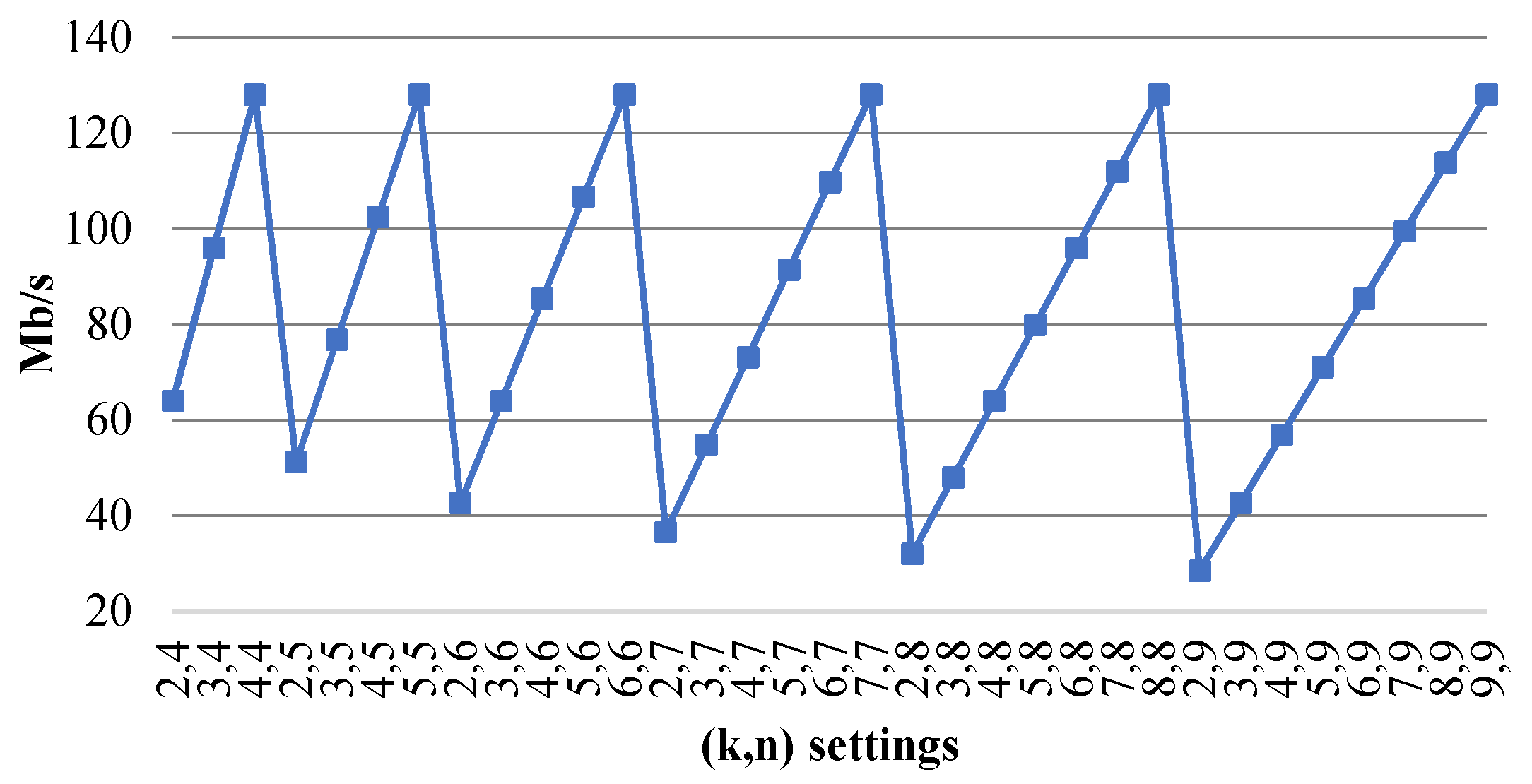
Figure 1 shows that the coding speed, $V_C$, versus $\left(k,n\right)$ parameters was a saw type. Picks were achieved for the schemes $\left(n, n\right)$, and minimums were achieved for $\left(2, n\right)$. The user can select the required parameters to obtain the required speed.

Figure 1. $V_C$ of a sPRNS versus $\left(k,n\right)$.

Figure 2 shows the coding speed, $V_C$, (Mb/s) of PRNS and RRNS. We can see that the coding speed of PRNS was higher than RRNS for all parameters.

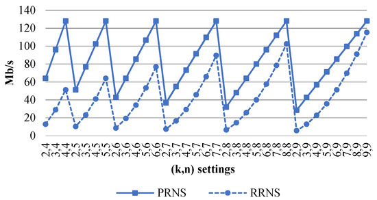
Figure 2. The $V_C$ of a PRNS and an RRNS versus $\left(k,n\right)$.

The PRNS operations on$GF\left(2^m\right)$ did not require the transfer of values from the lowest to the highest term. Consequently, the time complexity of the division remainder decreased compared to the arithmetic operations of RRNS performed over $GF\left(2^m\right)$.

4.2. PRNS Decoding Speed with Data Errors

To correct the $\lfloor r/2\rfloor$ errors with $r$ extra moduli, we used the projection method. To compute a projection, CRT with algorithmic complexity $O\left(D^2\right)$ required roughly $D^2=k^2·d^2$ bit operations. Since the number of projections was $C_n^{k+\lfloor \frac{r}{2}\rfloor }$, to detect and localize an error, we needed $C_n^{k+\lfloor \frac{r}{2}\rfloor }·k^2·d^2$ bit operations.

Hence

$$2^{23}·\frac{C_n^{k+\lfloor \frac{r}{2}\rfloor }·k^2·d^2}{k·d}=2^{23}·C_n^{k+\lfloor \frac{r}{2}\rfloor }·d·k$$

bit operations were required to code 1 Mb with the worst-case decoding speed, $V_D$.

$$V_D=\frac{2^{30}}{2^{23}·C_n^{k+\lfloor \frac{r}{2}\rfloor }·d·k}=\frac{2^7}{C_n^{k+\lfloor \frac{r}{2}\rfloor }·d·k}.$$

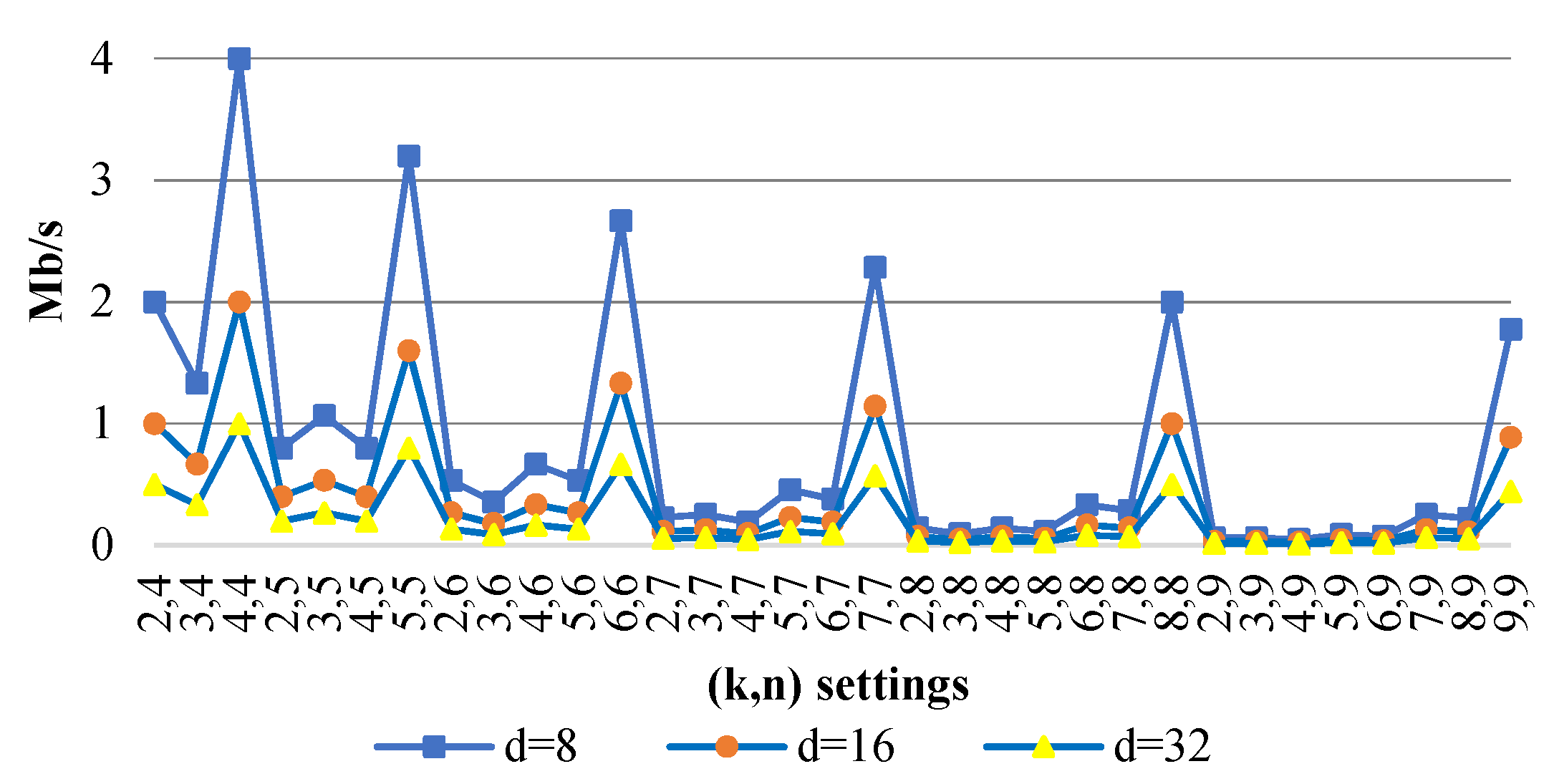
Figure 3 shows the data decoding speed, $V_D$, varying PRNS parameters for $d=\left\{8, 16, 32\right\}$.

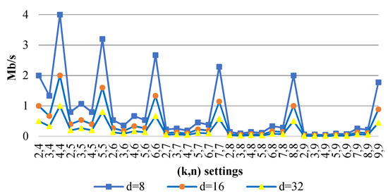
Figure 3. $V_D$ of a PRNS (Mb/s) versus $\left(k,n\right)$ for $d=\left\{8, 16, 32\right\}$.

We can see that the computational complexity of PRNS, when an error was localized, was higher than that of RRNS. Hence, the PRNS decoding speed was less than for RRNS.

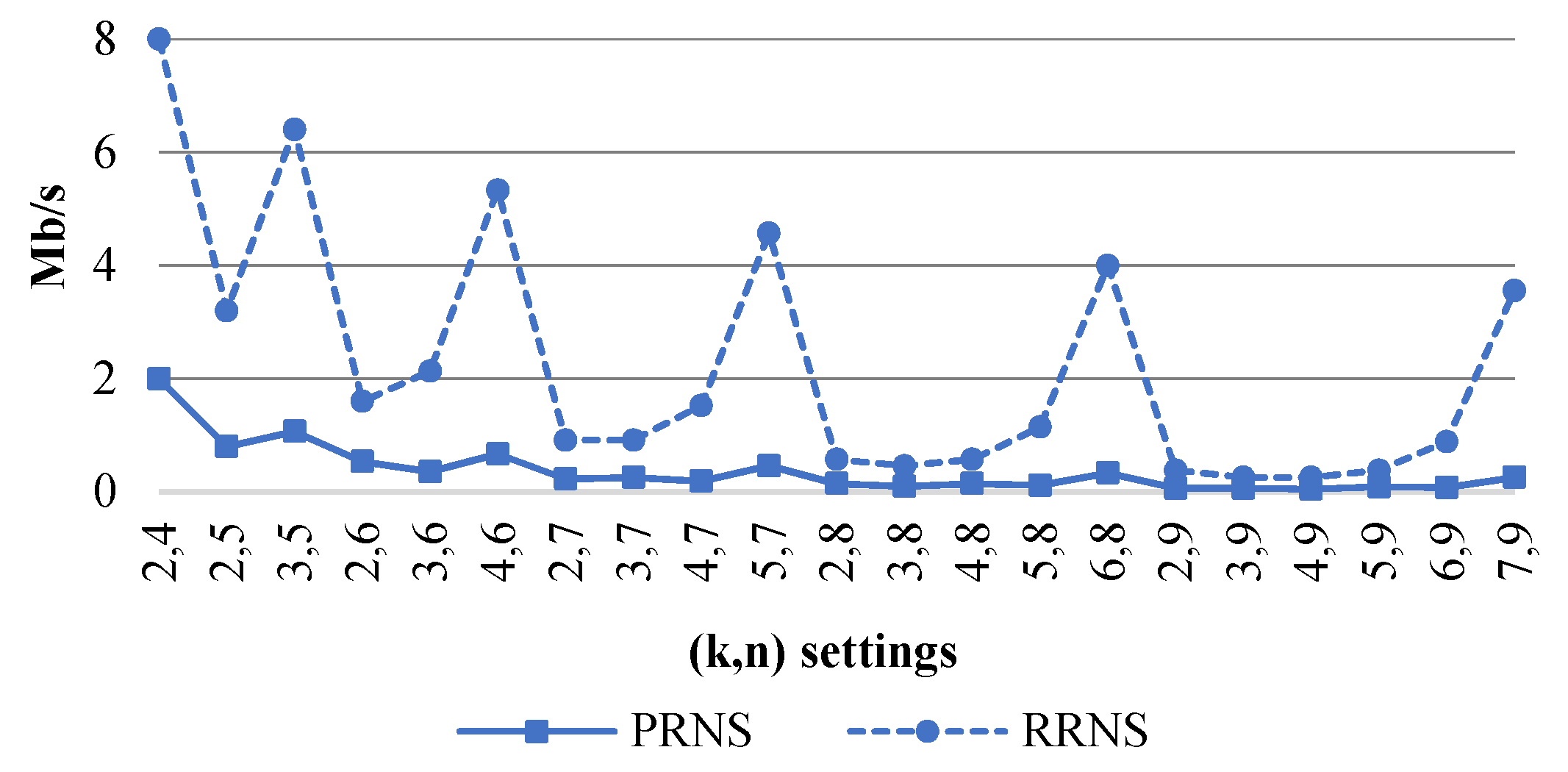
Figure 4 shows the PRNS and RRNS decoding speeds, $V_D$ (Mb/s), of the worst-case scenario with the maximum number of errors.

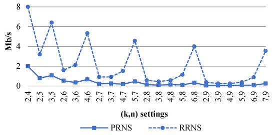
Figure 4. $V_D$ of a PRNS and an RRNS with the maximum number of errors versus $\left(k,n\right)$ for $d=8$.

The approximation of the rank of the PRNS number was used to increase this speed (Section 5).

4.3. Data Redundancy

To prevent system operation disruption in the case of technical failures, disasters, and cyber-attacks by maintaining a continuity of service data redundancy is very important.

The input polynomial is $A_P\left(x\right)$, where $\mathrm{deg} A_P\left(x\right)<D$. Hence, the total input volume approximately equals $D$. The number of bits needed for residues is equal to $\widehat{D}$ in the worst case. The data redundancy degradation is the ratio of the coded data size to the original minus 1:

$$R=\frac{\widehat{D}}{D}-1.$$

Let us select $m_i\left(x\right)$ so that $a_i\left(x\right)$ uses at most $d_1=d_2=\dots =d_n=d$ bits or one word. Hence, the redundancy is roughly $n/k-1$.

$$R=\frac{\widehat{D}}{D}-1=\frac{n·d}{k·d}-1=\frac{n-k}{k}.$$

Figure 5 shows the redundancy versus the PRNS parameters. We can see that the minimum values are for $\left(n,n\right)$, where $n=4, 5,\dots ,9$. These values are less than those of the Bigtable system $\left(\lceil \left(n+1\right)/3\rceil ,n\right)$.

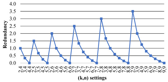
Figure 5. Data redundancy versus PRNS settings $\left(k,n\right)$.

PRNS reduces data redundancy compared to numerical RNS, because the degree of the polynomial (residue) is strictly less than the degree of the divisor. We demonstrate this in the following example.

Example 1.

Let us consider a ($4,4$) scheme with PRNS. Let the moduli be  $m_1\left(x\right)=x^8+x^4+x^3+x+1$, $m_2\left(x\right)=x^8+x^4+x^3+x^2+1$, $m_3\left(x\right)=x^8+x^5+x^3+x+1$, and $m_4\left(x\right)=x^8+x^5+x^3+x^2+1$. In this case, the dynamic range is:

$$\begin{gathered} M\left(x\right)={\displaystyle \prod }_{i=1}^4{m}_i\left(x\right)=x^{32}+x^{26}+x^{24}+x^{23}+x^{21}+ \\ {x}^{19}+x^{18}+x^{16}+x^{11}+x^{10}+x^9+x^5+x^4+x^2+1 \end{gathered}$$

Let $A_P\left(x\right)=x^{31}+x^{16}+x^{15}+x^{14}+1$, and it has 32 bits. $A_P\left(x\right)$has the following representation:

$$A_P\left(x\right)\stackrel{PRNS}{\to }{A}_{PRNS}=\left(a_1\left(x\right), a_2\left(x\right), a_3\left(x\right), a_4\left(x\right)\right),$$

where $a_1\left(x\right)={\left|A\left(x\right)\right|}_{m_1\left(x\right)}=x^7+x^4+x^3$, $a_2\left(x\right)={\left|A\left(x\right)\right|}_{m_2\left(x\right)}=x^7+x^5+x^4+x^3$, $a_3\left(x\right)={\left|A\left(x\right)\right|}_{m_3\left(x\right)}=x^7+x^4+x^3+x+1$, $a_4\left(x\right)={\left|A\left(x\right)\right|}_{m_4\left(x\right)}=x^7+x^6+x^3+x$, $a_1\left(x\right)$, $a_2\left(x\right)$, $a_3\left(x\right)$, and $a_4\left(x\right)$ are seventh-degree polynomials of 8 bits.

Therefore, the redundancy degradation is $4\times \frac{8}{32}-1=0$.

5. Approximation of the Rank of the PRNS Number

5.1. Rank

Reducing the computational complexity of the decoding algorithm is of the utmost interest. One possible approach is to approximate the value of the AR [15].

In CRT, the rank $r_A\left(x\right)$ of $A_{PRNS}$ is determined by Equation (2). It is used to restore $A_P\left(x\right)$ from residues:

$$A_P\left(x\right)={{\displaystyle \sum }}_{i=1}^k{M}_i\left(x\right)·O_i\left(x\right)·a_i\left(x\right)-r_A\left(x\right)·M\left(x\right)$$

(2)

Hence, $r_A\left(x\right)=\lfloor {{\displaystyle \sum }}_{i=1}^k\frac{O_i\left(x\right)}{m_i\left(x\right)}{a}_i\left(x\right)\rfloor , M\left(x\right)={{\displaystyle \prod }}_{i=1}^k{m}_i\left(x\right), M_i\left(x\right)=\frac{M\left(x\right)}{m_i\left(x\right)}$ and $O_i\left(x\right)={\left|M_i^{-1}\left(x\right)\right|}_{m_i\left(x\right)}$ for all $i=1,2,\dots ,k.$

$r_A\left(x\right)$ is the quotient of dividing ${{\displaystyle \sum }}_{i=1}^k{M}_i\left(x\right)·O_i\left(x\right)·a_i\left(x\right)$ by $M\left(x\right)$ in PRNS representation. Its calculation includes an expensive operation of the Euclidean division. Instead of computing the rank $r_A\left(x\right)$, we calculate an approximation of the rank, $R_A\left(x\right)$, based on the approximate method and modular adder, which decreases the complexity:

$$R_A\left(x\right)=\lfloor {{\displaystyle \sum }}_{i=1}^k{b}_i\left(x\right)a_i\left(x\right)/x^N\rfloor ,$$

(3)

where$b_i\left(x\right)=\lceil O_i\left(x\right)·x^N/m_i\left(x\right)\rceil .$

This method reduces the number of projections and replaces the computationally complex operation of the division of polynomials with the remainder by taking the division of a polynomial by the monomial $x^N$. The complexity is reduced from $O\left(D^2\right)$ to $O\left(D·\log D\right)$.

Theorem 1 shows that $R_A\left(x\right)$ and $r_A\left(x\right)$ are equal. It provides the theoretical basis for our approach.

Theorem 1.

If $N=\underset{i\in \overline{1,n}}{\max }\mathrm{deg}{m}_i\left(x\right)$, then $r_A\left(x\right)=R_A\left(x\right)$.

The proof is described in Appendix A.

The algorithmic complexity of the rank of $r_A\left(x\right)$ based on the Theorem 1 is $O \left(d·\log k\right)$. Since the coefficients $b_i\left(x\right)$ are of degree $d$, we can compute $A$ efficiently and reduce the computational complexity of the decoding from $O\left(D^2\right)$ down to $O \left(D·\log D\right).$ Computation of ${{\displaystyle \sum }}_{i=1}^k{M}_i\left(x\right)·O_i\left(x\right)·a_i\left(x\right)$ can be performed in parallel with the computation of $R_A\left(x\right)$.

5.2. AR-PRNS Decoding Speed with Data Errors

In the previous section, we described finding the error using AR to increase the decoding speed.

To detect and localize $\lfloor r/2\rfloor$ errors using the syndrome method, it is necessary to pre-compute a table consisting of $\lfloor r/2\rfloor ·d$ possible syndromes (rows). The maximum number of bit errors is $\lfloor r/2\rfloor ·d$. Each syndrome indicates the localization of errors. To find the syndrome in the table by binary search, we need ${\log }_2(\lfloor r/2\rfloor ·d)·r·d$ bit operations. To code 1 Mb, we need

$$2^{23}\left({\log }_2\left(\lfloor r/2\rfloor ·d\right)·r·d+\lfloor r/2{\rfloor }^2·d^2\right)/\left(k·d \right)=2^{23}·\left({\log }_2\left(\lfloor r/2\rfloor ·d\right)·r+\lfloor r/2{\rfloor }^2·d\right)/k$$

bit operations. Therefore, the AR-PRNS decoding speed in the worst case is

$$V_{D\_AR\_PRNS}=\frac{2^{30}·k}{2^{23}·\left({\log }_2\left(\lfloor \frac{r}{2}\rfloor ·d\right)·r+\lfloor r/2{\rfloor }^2·d\right)}=\frac{2^7·k}{{\log }_2\left(\lfloor \frac{r}{2}\rfloor ·d\right)·r+\lfloor r/2{\rfloor }^2·d}.$$

To detect and correct at least one error, $k$ has to satisfy the inequality $k\le n-2$.

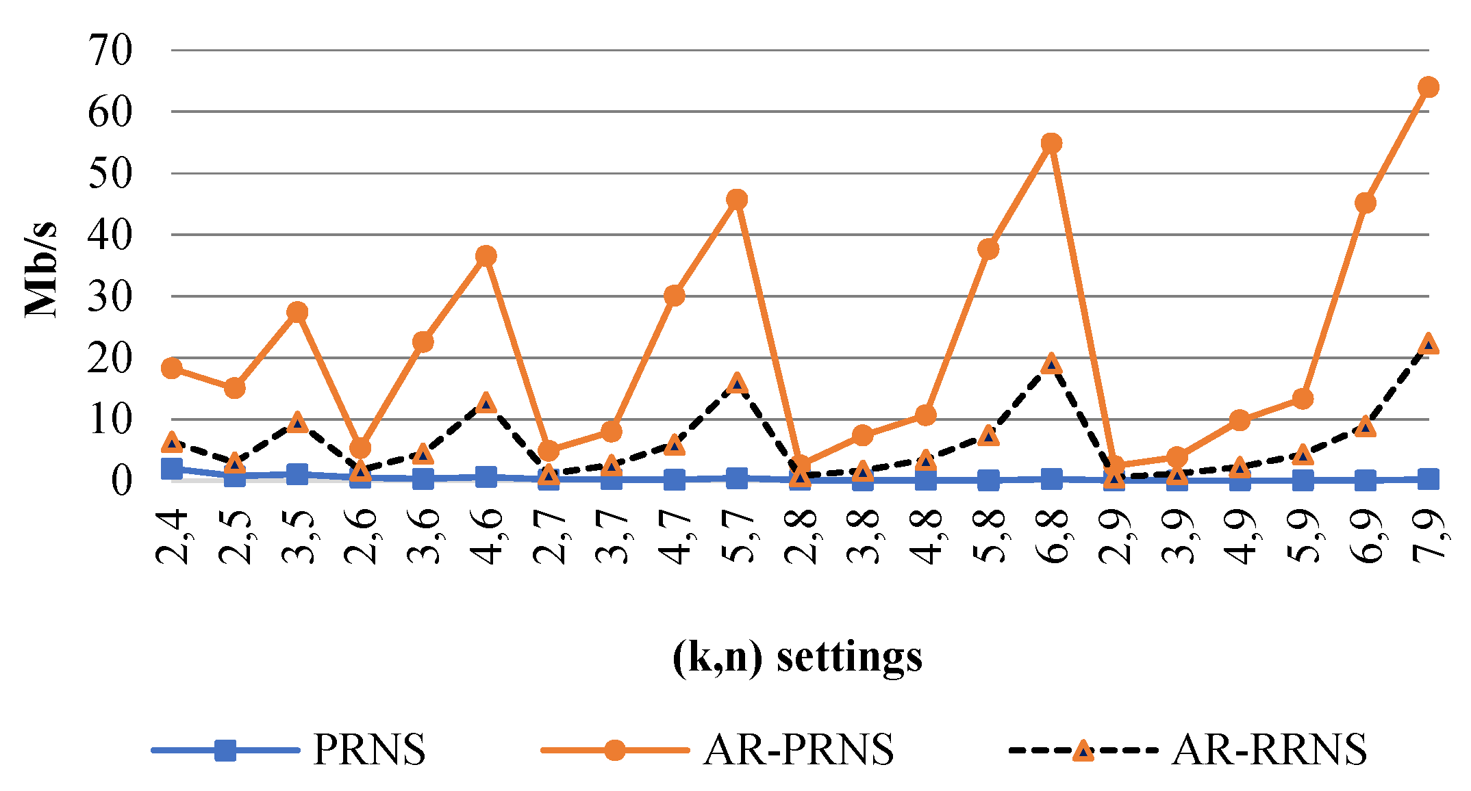
Figure 6 shows the decoding speeds of PRNS, AR-RRNS, and AR-PRNS depending on the parameters that satisfy this condition. We can see that AR-PRNS outperformed the others by almost three times.

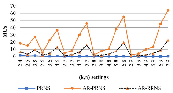
Figure 6. The decoding speed (Mb/s) of a PRNS, AR-PRNS, and AR-RRNS versus the settings $\left(k,n\right)$ in the worst-case scenario with the maximum number of errors for $d=8$.

6. Entropy Polynomial Error Correction Code

We propose a novel En-AR-PRNS method for data decoding that uses AR for decoding speed improvement and entropy for reliability improvement. We show that the entropy concept in PRNS can correct more errors than a traditional threshold-based PRNS.

First, ${{\displaystyle \sum }}_{i=1}^n{\widehat{M}}_i\left(x\right)·{\hat{O}}_i\left(x\right)·a_i\left(x\right)$ can be represented in the form:

$${{\displaystyle \sum }}_{i=1}^n{\widehat{M}}_i\left(x\right)·{\hat{O}}_i\left(x\right)·a_i\left(x\right)=A_P\left(x\right)+r_A\left(x\right)·\hat{M}\left(x\right),$$

(4)

Assume that an error has the following form:

$$E_P\left(x\right)\stackrel{PRNS}{\to }{E}_{PRNS}=\left(e_1\left(x\right),e_2\left(x\right),\dots ,e_n\left(x\right)\right).$$

Then, instead of $A_{PRNS}$, we have ${\overline{A}}_{PRNS}=A_{PRNS}+E_{PRNS}$.

Using (4), we have:

$${{\displaystyle \sum }}_{i=1}^n{\widehat{M}}_i\left(x\right)·{\hat{O}}_i\left(x\right)·(a_i\left(x\right)+e_i\left(x\right))=A_P\left(x\right)+E_P\left(x\right)+r_A\left(x\right)·\widehat{M}\left(x\right)+r_E\left(x\right)·\hat{M}\left(x\right)$$

Without loss of generality, we assume that moduli are in ascending order, i.e., $\mathrm{deg}{m}_1\le \mathrm{deg}{m}_2\le \dots \le \mathrm{deg}{m}_n$.

Since $k$ moduli are included in the dynamic range and $r$ is redundant (control moduli), where $k+r=n$, $\mathrm{deg}{A}_P\left(x\right)<D=\mathrm{deg}{{\displaystyle \prod }}_{i=1}^k{m}_i\left(x\right)={{\displaystyle \sum }}_{i=1}^k{d}_i.$ Since an error is of the form $E\left(x\right)=\beta \left(x\right){\hat{M}}_I\left(x\right)$, where ${\hat{M}}_I\left(x\right)={{\displaystyle \prod }}_{i\in I }{m}_i\left(x\right)$, $\beta \left(x\right)$ is a nonzero polynomial, and $I$ is the tuple of residues without errors.

If $I$ is not an empty tuple and $\mathrm{deg}{\hat{M}}_I\left(x\right)\ge {{\displaystyle \sum }}_{i=1}^k{d}_i$, then an error can be detected, since $\mathrm{deg}{E}_P\left(x\right)\ge {{\displaystyle \sum }}_{i=1}^k{d}_i$.

6.1. Entropy in PRNS

According to CRT, $A_P\left(x\right)$ is a polynomial over the binary field of degree less than $D={{\displaystyle \sum }}_{i=1}^k{d}_i$. Therefore, $A_P\left(x\right)$ can have $2^D$ different values. Following Kolmogorov (1965) [36] and Ivanov et al. (2019) [37], we can state that the entropy of $A_P\left(x\right)$ is equal to:

$$H\left(A_P\left(x\right)\right)={\log }_2{2}^D=D={{\displaystyle \sum }}_{i=1}^k{d}_i,$$

(5)

If $i\in \left[1,n\right]$ and $a_i\left(x\right)={\left|A_P\left(x\right)\right|}_{m_i\left(x\right)}$, then the entropy of $a_i\left(x\right)$ is equal to $d_i$:

$$H\left(a_i\left(x\right)\right)=d_i$$

(6)

Hence, the residue $a_i\left(x\right)$ carries some information of $A$. If the entropy $d_i=0$, the residue does not carry information about $A_P\left(x\right)$. In another extreme, if $d_i=D$, the residue equals to $A_P\left(x\right)$. From Equation (5) and Equation (6), it follows that:

$${{\displaystyle \sum }}_{i\in I}{d}_i\ge {{\displaystyle \sum }}_{i=1}^k{d}_i.$$

(7)

If Equation (7) is satisfied, the amount of known information is greater than or equal to the initial information. Hence, we can restore $A_P\left(x\right)$, where $I$ is a tuple of residues without error.

From the information theory point of view, the entropy of the residue $a_i\left(x\right)$ can be viewed as a measure of how close it is to the minimal entropy case. Hence, it measures the amount of information that $a_i\left(x\right)$ carries from $A_P\left(x\right)$. The maximal entropy corresponds to a non-coding–non-secure case.

Using an entropy-based approach, we can verify the obtained result for its correctness using the following theorem.

Theorem 2.

Let $m_1\left(x\right), m_2\left(x\right),\dots ,m_n\left(x\right)$be the PRNS moduli n-tuple, ${\overline{A}}_P\left(x\right)\stackrel{PRNS}{\to }{\overline{A}}_{PRNS}=\left({\overline{a}}_1\left(x\right),{\overline{a}}_2\left(x\right),\dots ,{\overline{a}}_n\left(x\right)\right)$, where $r$control moduli,$k=n-r$, and $\overline{I}$is a tuple of residues with an error. If

$${{\displaystyle \sum }}_{i\in \overline{I}}{d}_i\le {{\displaystyle \sum }}_{i=1}^r{d}_{k+i},$$

(8)

an error can be detected.

Proof. 

Let us consider two cases: when there is an error and when there is no error.

Case 1. If $\overline{I}$ is an empty tuple, then there are no errors and $A_P\left(x\right)$ can be calculated using (1).

Case 2. If $\overline{I}$ is not an empty tuple and it satisfies the condition (8), then we show that $\mathrm{deg}{\overline{A}}_P\left(x\right)>\mathrm{deg}{A}_P\left(x\right)$, where ${\overline{A}}_P\left(x\right)=A_P\left(x\right)+E_P\left(x\right)$. Due to the fact that $E_P\left(x\right)=\beta \left(x\right){{\displaystyle \prod }}_{i\in I}{m}_i\left(x\right),$ where $\beta \left(x\right)\ne 0$, we have:

$$\mathrm{deg}{E}_P\left(x\right)=\mathrm{deg}\beta \left(x\right)+{{\displaystyle \sum }}_{i\in I}{d}_i,$$

(9)

Given that ${{\displaystyle \sum }}_{i\in I}{d}_i={{\displaystyle \sum }}_{i=1}^n{d}_i-{{\displaystyle \sum }}_{i\in \overline{I}}{d}_i$, then Equation (9) takes the following form:

$$\mathrm{deg}{E}_P\left(x\right)=\mathrm{deg}\beta \left(x\right)+{{\displaystyle \sum }}_{i=1}^n{d}_i-{{\displaystyle \sum }}_{i\in \overline{I}}{d}_i,$$

(10)

Substituting the condition of the theorem ${{\displaystyle \sum }}_{i\in \overline{I}}{d}_i\le {{\displaystyle \sum }}_{i=1}^r{d}_{k+i}$ into Equation (10), we obtain that $\mathrm{deg}{E}_P\left(x\right)$ satisfies the following inequality:

$$\mathrm{deg}{E}_P\left(x\right)\ge \mathrm{deg}\beta \left(x\right)+{{\displaystyle \sum }}_{i=1}^n{d}_i-{{\displaystyle \sum }}_{i=1}^r{d}_{k+i},$$

(11)

Because ${{\displaystyle \sum }}_{i=1}^n{d}_i-{{\displaystyle \sum }}_{i=1}^r{d}_{k+i}={{\displaystyle \sum }}_{i=1}^k{d}_i$, then Equation (11) takes the following form:

$$\mathrm{deg}{E}_P\left(x\right)\ge \mathrm{deg}\beta \left(x\right)+{{\displaystyle \sum }}_{i=1}^k{d}_i.$$

(12)

Given that $\mathrm{deg}\beta \left(x\right)\ge 0$, then from the inequality (12), it follows $\mathrm{deg}{E}_P\left(x\right)\ge {{\displaystyle \sum }}_{i=1}^k{d}_i$. Because $\mathrm{deg}{A}_P\left(x\right)<{{\displaystyle \sum }}_{i=1}^k{d}_i$ and $\mathrm{deg}{\overline{A}}_P\left(x\right)=\mathrm{deg}E\left(x\right)\ge {{\displaystyle \sum }}_{i=1}^k{d}_i$, an error is detected. The theorem is proved. □

Example 2.

(see Appendix B) considers the case when the degrees of control moduli are less than the degrees of working moduli so that we can find an error in the remainder of the division by the working moduli.

Example 3 considers the case when one control modulo is used. We can detect two errors unlike one error in the traditional PRNS.

Example 3.

Let PRNS moduli tuple be $m_1\left(x\right)=x^2+x+1$, $m_2\left(x\right)=x^3+x+1$, $m_3\left(x\right)=x^3+x^2+1$, and $m_4\left(x\right)=x^6+x+1$, where $k=3$, $r=1,$and $n=3+1=4$. The dynamic range of PRNS is $M\left(x\right)=x^8+x^6+x^5+x^4+x^3+x^2+1$and $\widehat{M}\left(x\right)=x^{14}+x^{12}+x^{11}+x^{10}+x^7+x^6+x^2+x+1$.

Let $A_P\left(x\right)=x^7\stackrel{PRNS}{\to }\left(x, 1, 1, x^2+x\right)$. We consider three cases in which errors occurred on two shares.

Case A. If errors occurred in $a_1\left(x\right)$and $a_2\left(x\right)$, then the error vector had the following form: $E_{PRNS}=\left(1,1, 0,0\right).$

$${\overline{A}}_{PRNS}=A_{PRNS}+E_{PRNS}=\left(x+1, 0, 1, x^2+x\right).$$

Because ${{\displaystyle \sum }}_{j\in {\overline{I}}_A}{d}_j=d_1+d_2=\mathrm{deg}{m}_1\left(x\right)+\mathrm{deg}{m}_2\left(x\right)=5$and ${{\displaystyle \sum }}_{i=1}^r{d}_{k+i}=d_4=\mathrm{deg}{m}_4\left(x\right)=6$, the condition of Theorem 2 (see Equation (8)) is satisfied, and errors can be detected.

Case B. If errors occurred in $a_1\left(x\right)$and $a_3\left(x\right)$, then the error vector is $E_{PRNS}=\left(1,0, 1,0\right)$; hence, ${\stackrel{=}{A}}_{PRNS}=A_{PRNS}+E_{PRNS}=\left(x+1, 1, 0, x^2+x\right)$. Because ${{\displaystyle \sum }}_{j\in {\overline{I}}_B}{d}_j=d_1+d_3=\mathrm{deg}{m}_1\left(x\right)+\mathrm{deg}{m}_3\left(x\right)=5$and ${{\displaystyle \sum }}_{i=1}^r{d}_{k+i}=d_4=\mathrm{deg}{m}_4\left(x\right)=6$, the condition of Theorem 2 (see Equation (8)) is satisfied, and errors can be detected.

Case C. If an error occurred in $a_2\left(x\right)$and $a_3\left(x\right)$then the error vector is $E_{PRNS}=\left(0,1, 1,0\right)$and ${\tilde{A}}_{PRNS}=A_{PRNS}+E_{PRNS}=\left(x, 0,0, x^2+x\right)$. Because ${{\displaystyle \sum }}_{j\in {\overline{I}}_C}{d}_j=d_2+d_3=\mathrm{deg}{m}_2\left(x\right)+\mathrm{deg}{m}_3\left(x\right)=6$and ${{\displaystyle \sum }}_{i=1}^r{d}_{k+i}=d_4=\mathrm{deg}{m}_4\left(x\right)=6$, the condition of Theorem 2 (see Equation (8)) is satisfied, and an error can be detected.

Let us show how an error is detected.

First, we calculated the PRNS constants ${\widehat{M}}_i\left(x\right)=\widehat{M}\left(x\right)/m_i\left(x\right)$.

$${\widehat{M}}_1\left(x\right)=x^{12}+x^{11}+x^{10}+x^9+x^8+x^6+1, {\widehat{M}}_2\left(x\right)=x^{11}+x^7+x^5+x^2+1,$$

$${\widehat{M}}_3\left(x\right)=x^{11}+x^{10}+x^4+x+1, {\widehat{M}}_4\left(x\right)=x^8+x^6+x^5+x^4+x^3+x^2+1;$$

$${\left|{\widehat{M}}_1^{-1}\left(x\right)\right|}_{m_1\left(x\right)}=x+1, {\left|{\widehat{M}}_2^{-1}\left(x\right)\right|}_{m_2\left(x\right)}=x, {\left|{\widehat{M}}_3^{-1}\left(x\right)\right|}_{m_3\left(x\right)}=x,$$

$${\left|{\widehat{M}}_4^{-1}\left(x\right)\right|}_{m_4\left(x\right)}=x^5+x^2+x.$$

Third, we compute ${\overline{A}}_P\left(x\right)$, ${\stackrel{=}{A}}_P\left(x\right)$, and ${\tilde{A}}_P\left(x\right)$, using Equation (1).

$${\overline{A}}_P\left(x\right)=x^{13}+x^{12}+x^3+1, {\stackrel{=}{A}}_P\left(x\right)=x^{13}+x^{12}+x^{11}+x^8+x^6+x^5+x^2+1,$$

$${\tilde{A}}_P\left(x\right)=x^{11}+x^8+x^7+x^6+x^5+x^3+x^2.$$

Finally, we determine whether ${\overline{A}}_P\left(x\right)$, ${\stackrel{=}{A}}_P\left(x\right)$, and ${\tilde{A}}_P\left(x\right)$have errors.

Case A. Because $\mathrm{deg}{\overline{A}}_P\left(x\right)=13>\mathrm{deg}M\left(x\right)=8$, then ${\overline{A}}_P\left(x\right)$contains an error.

Case B. Because $\mathrm{deg}{\stackrel{=}{A}}_P\left(x\right)=13>\mathrm{deg}M\left(x\right)=8$, then ${\stackrel{=}{A}}_P\left(x\right)$contains an error.

Case C. Because $\mathrm{deg}{\tilde{A}}_P\left(x\right)=11>\mathrm{deg}M\left(x\right)=8$, then ${\tilde{A}}_P\left(x\right)$contains an error.

To detect an error, we use Theorem 2. To localize and correct the error, we modify the maximum likelihood decoding (MLD) method from Goh and Siddiqi (2008) [38].

6.2. MLD Modification

To correct errors, we need tuple $I$ residues, where ${{\displaystyle \sum }}_{i\in I}{d}_i>D$. One of the ways to select them from all correct residues is the MLD method.

In the process of localization and correction of errors, we calculate the tuple $V$ of possible candidates, ${\overline{A}}_P\left(x\right)$, satisfying the condition $\mathrm{deg}{\overline{A}}_P\left(x\right)<D$. Each of the possible ${\overline{A}}_P\left(x\right)$ is denoted by $V_P^l\left(x\right)$, that is:

$$V=\left\{V_P^1\left(x\right),V_P^2\left(x\right),\dots ,V_P^l\left(x\right),\dots ,V_P^{\lambda }\left(x\right)\right\}$$

where $\lambda$ is the total number of candidate ${\overline{A}}_P\left(x\right)$ that fall within the legitimate range, from which $A_P\left(x\right)$ is selected.

If their entropies equal $d_1=d_2=\dots =d_n$, then we can use the Hamming distance, $H_T^l$ (i.e., Hamming distance between $V_{PRNS}^l$ and vector ${\overline{A}}_{PRNS}$), of residues. $H_T^l$ is defined as the number of elements in which two vectors, $V_{PRNS}^l$ and ${\overline{A}}_{PRNS}$, differ.

But if we consider weighted error correction codes in which $d_1\ne d_2\ne \dots \ne d_n$, then the Hamming distance does not provide correct measurement, since residues carry a different amount of information about $A_P\left(x\right)$.

Let $m_1\left(x\right)$, $m_2\left(x\right)$,…, $m_n\left(x\right)$ be the PRNS moduli tuple:

$$V_P^l\left(x\right)\stackrel{PRNS}{\to }{V}_{PRNS}^l=\left(v_{l,1}\left(x\right),v_{l, 2}\left(x\right),\dots ,v_{l,n}\left(x\right)\right).$$

Let us calculate $H_W^l$ as the Hamming weight of $V_{PRNS}^l$ and ${\overline{A}}_{PRNS}$ using the following Algorithm 1.

Algorithm 1.$\mathrm{Calculation} H_W^l$.

Input:

${\overline{A}}_{PRNS}=\left({\overline{a}}_1\left(x\right),{\overline{a}}_2\left(x\right),\dots ,{\overline{a}}_n\left(x\right)\right)$

$V_{PRNS}^l=\left(v_{j,1}\left(x\right),v_{j, 2}\left(x\right),\dots ,v_{j,n}\left(x\right)\right)$

$h_E=\left(H\left(a_1^{\prime }\left(x\right)\right),H\left(a_2^{\prime }\left(x\right)\right),\dots ,H\left(a_n^{\prime }\left(x\right)\right)\right)$

Output$: H_W^l$.

$h\leftarrow \left(h_1,h_2,\dots ,h_n\right)$                $//$Hamming vector

for$i\leftarrow 1$to$n$

$\mathbf{if} v_{j, i}\left(x\right)={\overline{a}}_i\left(x\right)$ then

$h_i\leftarrow 0$

else

$h_i\leftarrow 1$

end if

end for

$\overline{h}\leftarrow \left({\overline{h}}_1,{\overline{h}}_2,\dots ,{\overline{h}}_n\right)$                   $//$Inverse of vector  $h$

for$i\leftarrow 1$to$n$

$\mathbf{if} h_i=0$ then

${\overline{h}}_i\leftarrow 1$            $//a_i\left(x\right)$ does not contain an error

else

${\overline{h}}_i\leftarrow 0$

end if

end for

$h_E\leftarrow \left(H\left({\overline{a}}_1\left(x\right)\right),H\left({\overline{a}}_2\left(x\right)\right),\dots ,H\left({\overline{a}}_n\left(x\right)\right)\right)\leftarrow \left(d_1,d_2,\dots ,d_n\right)$

$H_W^l\leftarrow H\left(V_{PRNS}^l\right) \leftarrow \overline{h}·h_E$

Return $H_W^l$

According to Algorithm 1, three steps are used to calculate $H_W^l$: First, similar to MLD, calculate the Hamming vector, $h=\left(h_1,h_2,\dots ,h_n\right)$, where $h_i\in \left\{0,1\right\}$. Second, calculate the inverse of the vector $h$, $\overline{h}=\left({\overline{h}}_1,{\overline{h}}_2,\dots ,{\overline{h}}_n\right)$, where ${\overline{h}}_i$ is equal to one if the remainder $a_i\left(x\right)$ does not contain an error, otherwise ${\overline{h}}_i$ is equal to zero. Third, calculate the amount of entropy, $H_W^l$, as a dot product of two vectors, $\overline{h}=\left({\overline{h}}_1,{\overline{h}}_2,\dots ,{\overline{h}}_n\right)$, and vectors consisting of the entropies of the remainders of the division, $a_i^{\prime }\left(x\right)$.

The idea is to calculate the amount of entropy, $H_W^l=H\left(V_{PRNS}^l\right)$, but not the number of errors, $H_T^l$, as in MLD. If the volume of correct data is greater than $D$, then according to Theorem 2, we can restore the value of $A_P\left(x\right)$.

Now, we can select $A_P\left(x\right)$ from all corrected $V_P^l\left(x\right)$. To this end, traditional MLD picks the candidate with the minimal Hamming distance. In our approach, the best candidate is the $V_P^l\left(x\right)$ with the maximal entropy, $H_W^l$.

Example 4.

Let PRNS moduli 4-tuple be $m_1\left(x\right)=x^2+x+1$, $m_2\left(x\right)=x^3+x+1$, $m_3\left(x\right)=x^3+x^2+1$, and $m_4\left(x\right)=x^6+x+1$, where $k=3$, $r=1,$and $n=k+r=4$.

Let the dynamic range $M\left(x\right)$and the full range of $\widehat{M}\left(x\right)$of PRNS be:

$$M\left(x\right)=x^8+x^6+x^5+x^4+x^3+x^2+1$$

and

$$\widehat{M}\left(x\right)=x^{14}+x^{12}+x^{11}+x^{10}+x^7+x^6+x^2+x+1$$

Let $A_P\left(x\right)=x^7\stackrel{PRNS}{\to }{A}_{PRNS}=\left(x, 1, 1, x^2+x\right)$and $E_{PRNS}=\left(1,0, 0,0\right)$, then ${\overline{A}}_{PRNS}=A_{PRNS}+E_{PRNS}=\left(x+1, 1, 1, x^2+x\right)$. There are three possible values of $V_P^l$that satisfy the condition $\mathrm{deg}{V}_P^l\left(x\right)<D={{\displaystyle \sum }}_{i=1}^k{d}_i$.

We present the calculation results in Table 2.

Table 2. $V$ with three candidates of $V_P^l\left(x\right)$.

$\mathit{j}$	${\mathit{V}}_{\mathit{P}}^{\mathit{l}}\left(\mathit{x}\right)\stackrel{\mathit{P}\mathit{R}\mathit{N}\mathit{S}}{\to }{\mathit{V}}_{\mathit{P}\mathit{R}\mathit{N}\mathit{S}}^{\mathit{l}}$	${\mathit{H}}_{\mathit{W}}^{\mathit{l}},$${\mathit{H}}_{\mathit{T}}^{\mathit{l}}$
1	$x^7\stackrel{PRNS}{\to }\left(x, 1, 1, x^2+x\right)$	$H_W^1=0+3+3+6=12$ $H_T^1=1+0+0+0=1$
2	$x^6+x^2+1\stackrel{PRNS}{\to }\left(x+1, 0, x+1, x^2+x\right)$	$H_W^2=2+0+0+6=8$ $H_T^2=0+1+1+0=2$
3	$x^7+x^6+x^5+x^4+x^3+x^2+x+1\stackrel{PRNS}{\to }\left(x+1, 1,1, x^5+x^4+x^3+x\right)$	$H_W^3=2+3+3+0=8$ $H_T^3=0+0+0+1=1$

If we use the MLD from Kolmogorov (1965) [36], then the tuple of possible recovering candidates $A_P\left(x\right)$ consists of two values $V_P^1\left(x\right)=x^7$ and $V_P^3\left(x\right)={{\displaystyle \sum }}_{i=0}^7{x}^i$ with the minimal Hamming distance. The proposed MLD modification for the error correction codes selects for maximal entropy. As we showed above, it allows us to determine the true result, $A_P\left(x\right)=V_P^1\left(x\right)=x^7\stackrel{PRNS}{\to }\left(x, 1, 1, x^2+x\right),$ unambiguously and correct the error. In classical PRNS, an error can be detected but not corrected.

7. Reliability

The detection of errors and failures in distributed storage and communication is mainly based on error correction codes, ECs, RCs, and modifications. In contrast to the existing methods, the PRNS method is simple and fast. However, it has one significant drawback: the limitation of detection and localization of errors. To overcome this limitation and increase the reliability, we propose an entropy-based approach to correct errors (see Section 6.1.).

Let ${\mathrm{Pr}}_i$ be the probability of error of data stored in the $i$-th cloud. It can be seen as the probability of unexpected and unauthorized modifications, falsifications, hardware and software failures, disk errors, integrity violations, denial of access or data loss, etc.

To correct errors, we have to take enough residues without errors. The data access structure is defined as a set of residues without errors allowing correct errors. It is defined as follows: ${\mathsf{\Gamma }}_{\mathit{En}-\mathit{AR}-\mathit{PRNS} }=\left\{I\right|{{\displaystyle \sum }}_{i\in I}{d}_i\ge D\}$.

Hence, the probability of information loss of an En-AR-PRNS is determined by (13).

$${\mathrm{Pr}}_{\mathit{En}-\mathit{AR}-\mathit{PRNS} }=1-{{\displaystyle \sum }}_{I\in \mathsf{\Gamma }}{{\displaystyle \prod }}_{i\in I}\left(1-{\mathrm{Pr}}_i\right){{\displaystyle \prod }}_{i\notin I}{\mathrm{Pr}}_i$$

(13)

To estimate the probability of $i$-th storage error (i.e., failure), ${\mathrm{Pr}}_i$, we used data from an analysis of the downtime of public cloud providers presented by CloudHarmony [12]. It monitors the health status of service providers by spinning up workload instances in public clouds and constantly pinging them. It does not present a complete insight into the types of failures due to the limited information obtained by monitoring; however, it serves as a valuable point of reliability analysis.

Table 3 describes the downtime, $T_D$ (in minutes per year), of eight cloud storage providers [39]. We calculated the ${\mathrm{Pr}}_i$ by the geometric probability definition (ratio of measures) ${\mathrm{Pr}}_i=T_D/525,600$, where $525,600=365\times 24\times 60$ is the number of minutes in a year. It included upload and download times (Tchernykh et al., 2018) [18].

Table 3. Characteristics of the clouds.

	Cloud	$$\begin{gathered} {\mathit{T}}_{\mathit{D}} \\ \left(\mathbf{min}\right) \end{gathered}$$	$\mathbf{P}{\mathbf{r}}_{\mathbf{i}}$	Speed (MB/s)		Latency (ms)
				Upload	Download
1	CenturyLink	1889	0.003594	3.04	4.56	277.25
2	IBM’s Cloud	1020	0.001941	3.51	4.05	80.42
3	Rackspace	770	0.001465	2.02	2.44	288.33
4	Digital Ocean	764	0.001454	5.08	5.82	87.50
5	Google	694	0.001320	2.68	4.23	201.58
6	Azure	649	0.001235	4.64	4.03	374.25
7	AWS	150	0.000285	2.63	2.9	281.17
8	Joyent	34	0.000065	2.13	3.11	390.83

Based on these probabilities, we can roughly estimate reliability by calculating the probability of information loss. In threshold PRNS, we lose data when at least $r+1$ storages have errors when we are not able to correct errors. In En-AR-PRNS, as we showed in Section 6, the entropy-based approach allows for correcting more errors.

Let us consider both approaches. Table 4 shows an example of data sharing in eight storages. Column $m_i\left(x\right)$ shows the eight moduli we used for coding, $H(a_i\left(x\right)$) is the entropy of obtained residues, and the Cloud column is the used storage.

Table 4. Data allocation based on PRNS.

i	${\mathit{m}}_{\mathit{i}}\left(\mathit{x}\right)$	$\mathit{H}\left({\mathit{a}}_{\mathit{i}}\left(\mathit{x}\right)\right)$	Cloud
1	$x^8+x^4+x^3+x+1$	8	CenturyLink
2	$x^8+x^4+x^3+x^2+1$	8	IBM’s Cloud
3	$x^8+x^5+x^3+x+1$	8	Rackspace
4	$x^8+x^5+x^3+x^2+1$	8	Digital Ocean
5	$x^8+x^5+x^4+x^3+1$	8	Google
6	$x^8+x^6+x^3+x^2+1$	8	Azure
7	$x^8+x^6+x^5+x+1$	8	AWS
8	$x^8+x^6+x^5+x^2+1$	8	Joyent

Due to the entropies and polynomial degrees being equal, the residues could be allocated based on the access speed, trustiness, etc., of the storages. In this case, the reliabilities of both the En-AR-PRNS and PRNS methods had no difference.

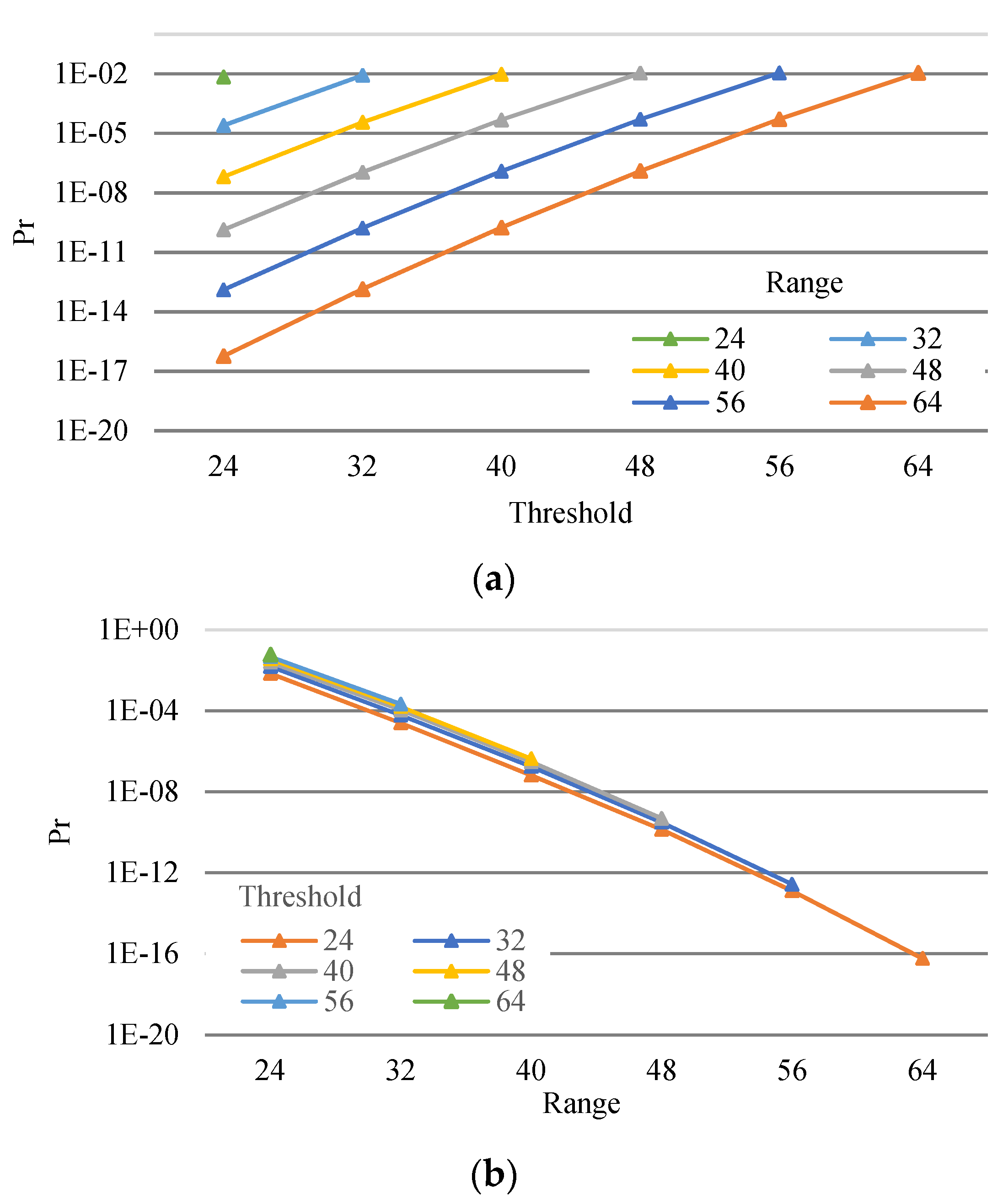
Figure 7 shows the probabilities of information loss. Figure 7a shows that this probability varied ranging from 24 (four storages) to 64 (eight storages) versus the threshold (dynamic range). Figure 7b shows this probability varying threshold from 24 to 64 versus the range.

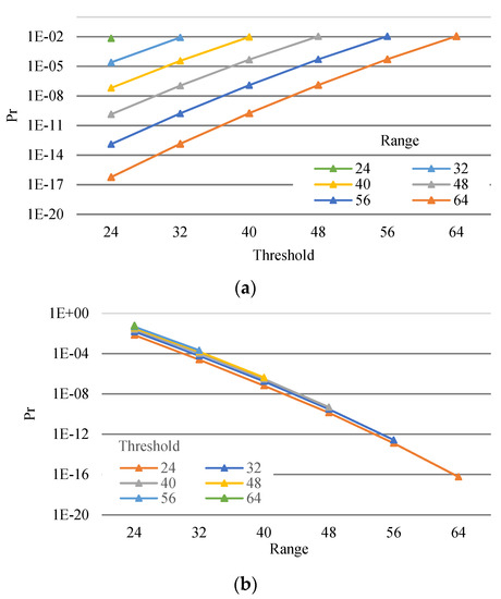
Figure 7. Probability of information loss of an En-AR-PRNS (a) and a PRNS (b).

We observed that:

• By reducing thresholds (i.e., increasing data redundancy), we reduced the probability of information loss (Figure 7a);
• By increasing the number of clouds (i.e., increasing the range), we reduced the probability of information loss (Figure 7a);
• Reduction in the information loss probability by increasing the range was approximately equal for all thresholds (see Figure 7b).

Example 5.

Let five cloud providers (i.e., Joyent, Azure, Google, Rackspace, and CenturyLink) be used for storage. The probabilities of errors and information loss were calculated using the data presented in [39] (see Table 5).

Table 5. Data allocation based on En-AR-PRNS.

$\mathit{i}$	${\mathit{m}}_{\mathit{i}}\left(\mathit{x}\right)$	$\mathit{H}\left({\mathit{a}}_{\mathit{i}}\left(\mathit{x}\right)\right)$	${\mathrm{Pr}}_{\mathit{i}}$	Cloud
1	$x^2+x+1$	2	0.003594	CenturyLink
2	$x^4+x+1$	4	0.001465	Rackspace
3	$x^4+x^3+1$	4	0.001320	Google
4	$x^4+x^3+x^2+x+1$	4	0.001235	Azure
5	$x^6+x+1$	6	0.000065	Joyent

Table 5 shows an example of the data sharing in these storage systems. The $m_i\left(x\right)$ column shows the five used moduli, the $H\left(a_i\left(x\right)\right)$ column shows the entropy of residues, and the Cloud column shows the storage provider.

Due to the fact that the entropies were different, we allocated the residue with the highest entropy, $H\left(a_i\left(x\right)\right)=6$, on storage with the lowest error probability, $i=5$. Then, we allocated three shares with entropy four on storages with the next smaller probabilities, $i=4, 3, 2$. Finally, we allocated the last share with entropy two on storage $i=1$.

For such an allocation, we used a PRNS with $k=3$ and $r=2$. The access structures ${\mathsf{\Gamma }}_{\mathit{En}-\mathit{AR}-\mathit{PRNS} }$ and ${\mathsf{\Gamma }}_{PRNS}$ included combinations of the residues (recovery cases) that could be used to recover original data.

${\mathsf{\Gamma }}_{PRNS}=${{1, 2, 3}, {1, 2, 4}, {1, 2, 5}, {1, 3, 4}, {1, 3, 5}, {1, 4, 5}, {2, 3, 4}, {2, 3, 5}, {2, 4, 5}, {3, 4, 5}, {1, 2, 3, 4}, {1, 2, 3, 5}, {1, 2, 4, 5}, {1, 3, 4, 5}, {2, 3, 4, 5}, {1, 2, 3, 4, 5}}.

${\mathsf{\Gamma }}_{\mathit{En}-\mathit{AR}-\mathit{PRNS} }=${{2, 5}, {3, 5}, {4, 5}} $\cup$ ${\mathsf{\Gamma }}_{PRNS}$.

${\mathsf{\Gamma }}_{\mathit{En}-\mathit{AR}-\mathit{PRNS} }$ had nineteen recovery cases and ${\mathsf{\Gamma }}_{PRNS}$ had sixteen cases. As we showed before, to restore data in a PRNS, we can have errors in two residues at most. In an En-AR-PRNS, we showed that, in some cases, we could restore data even with three residues have errors.

The probability of information loss calculated by (13) was ${\mathrm{Pr}}_{PRNS}=2.3\times {10}^{-8}$ and ${\mathrm{Pr}}_{\mathit{En}-\mathit{AR}-\mathit{PRNS} }=3.7\times {10}^{-9}$. Therefore, En-AR-PRNS improved the reliability of the storage by about $\frac{2.3·{10}^{-8}}{3.7·{10}^{-9}}\approx 6.2$ times using the same number of clouds with the same probability of errors for each provider.

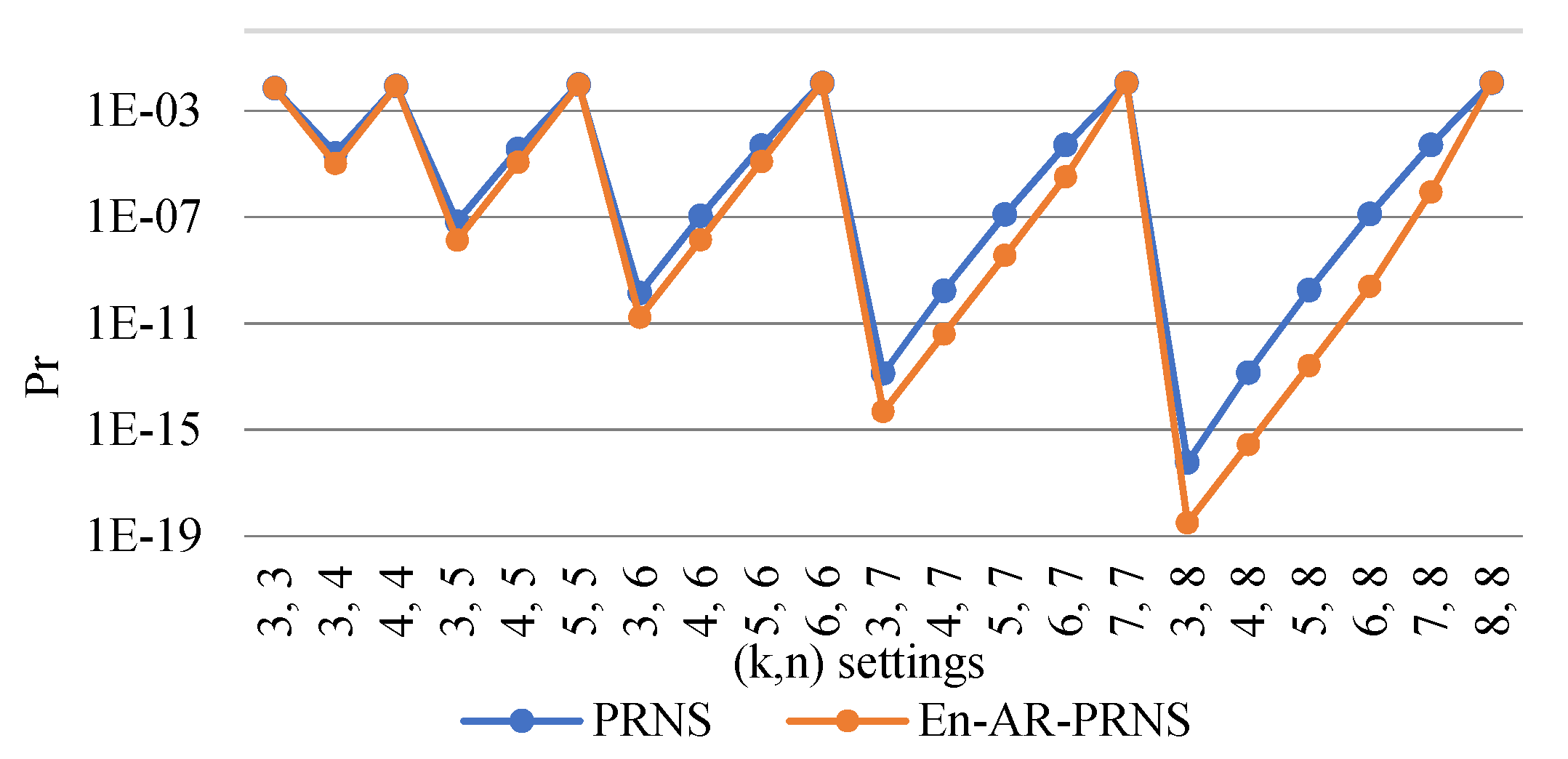
Now, let us compare the reliability of data storages based on PRNS and En-AR-PRNS with various $\left(k,n\right)$ settings. We defined the degree of residues as follows: $d_1=d_2=\dots =d_k=8$ and $d_{k+1}=d_{k+2}=\dots =d_n=16$. The probabilities of information loss of threshold PRNS and entropy-based PRNS on a logarithmic scale are presented in Figure 8.

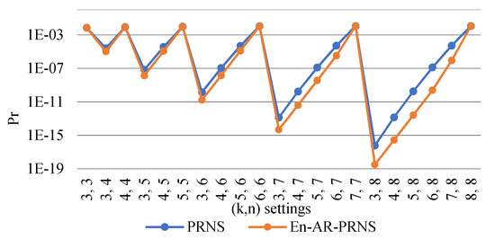
Figure 8. The probability of information loss of a threshold PRNS and an entropy-based PRNS.

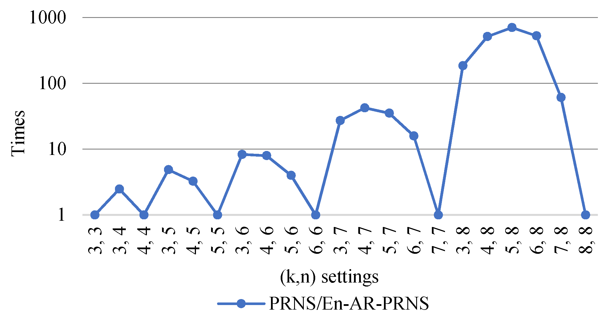
To show the advantage of an entropy-based approach, Figure 9 presents the reliability improvement of En-AR-PRNS over PRNS. We can see that the largest improvement was approximately eighty times for $\left(5, 8\right)$ settings. The top improvements were for $\left(3, 4\right), \left(3, 5\right), \left(3, 6\right), \left(4, 7\right), \mathrm{and} \left(5, 8\right)$.

Figure 9. Reliability improvement of En-AR-PRNS over PRNS.

We can conclude that for the same number of cloud providers, the probability of information loss for En-AR-PRNS was much lower than for PRNS.

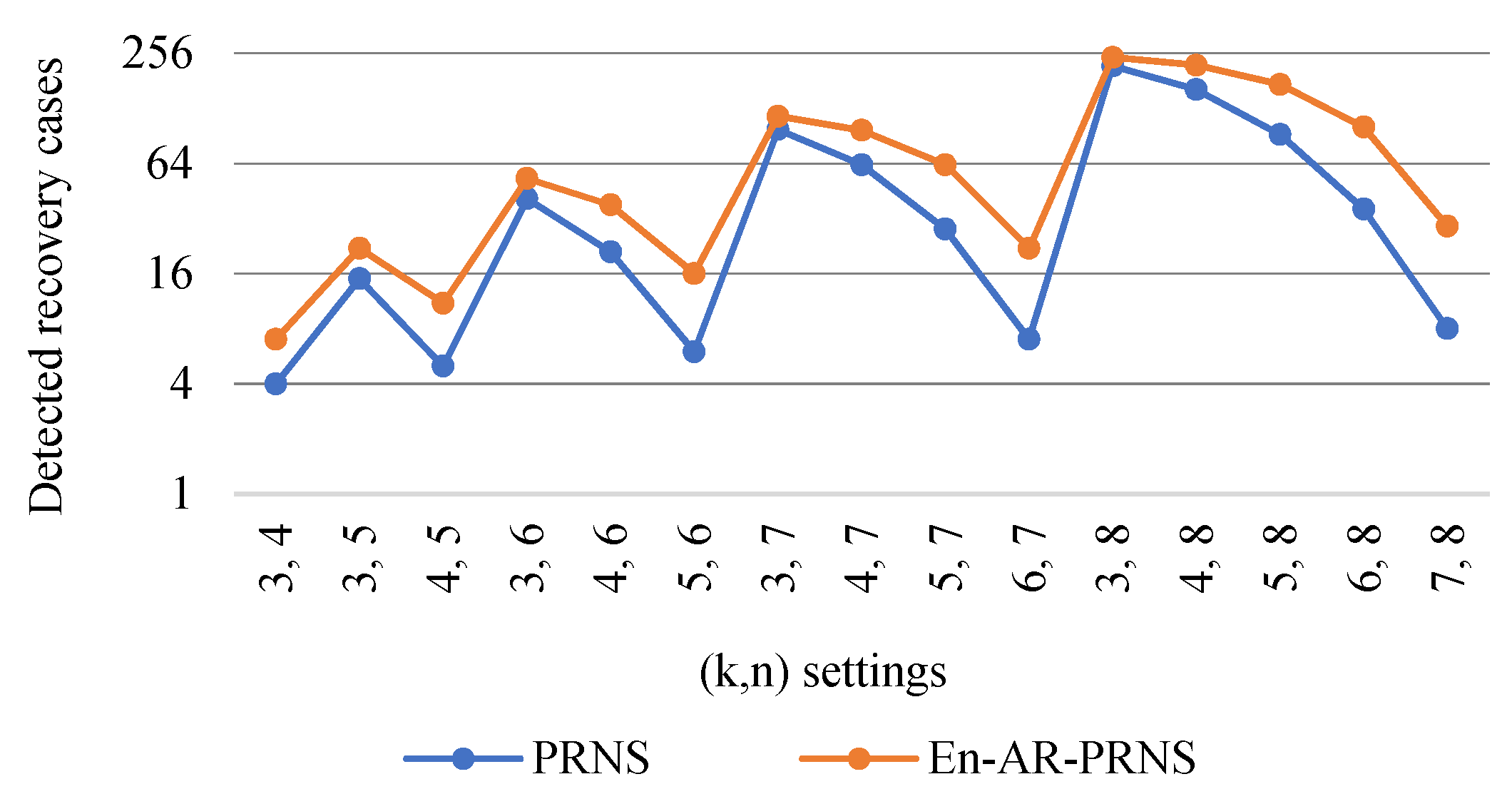
Now, we show how many recovery cases can be detected and corrected by both approaches.

Figure 10 shows the number of recovery cases found by an En-AR-PRNS and a PRNS. For instance, for $\left(3, 4\right)$ settings, the PRNS could detect only one error in shares $i=1, 2, 3, 4$. The En-AR-PRNS could detect the same errors and three more cases when detecting errors in two shares, for a total of seven cases.

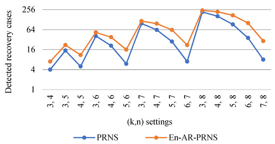
Figure 10. Number of recovery cases detected by the En-AR-PRNS and the PRNS.

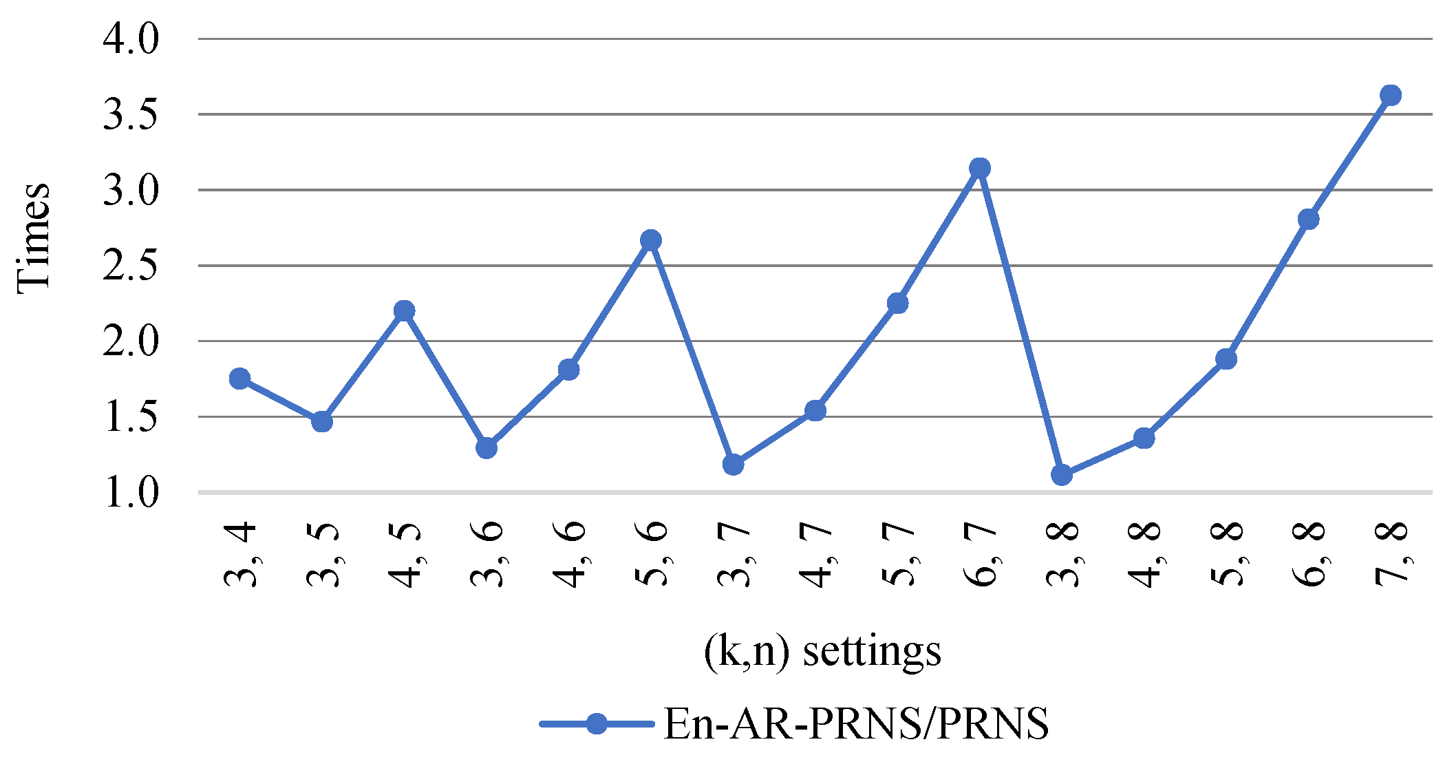
Figure 11 shows how many times the En-AR-PRNS outperformed the PRNS in error detection. We can see that for $\left(7, 8\right)$ settings, the En-AR-PRNS outperformed the PRNS by 3.6 times.

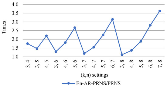
Figure 11. Improvement of number of recovery cases detected by En-AR-PRNS over PRNS.

An En-AR-PRNS detects and corrects more errors than classical methods in a PRNS. Table 6 shows the comparative analysis of the methods.

Table 6. Comparison of multiple residue digit error detection and correction algorithms.

Algorithm	Number of Errors Correctable	Number of Errors Detected	Output Domain	Method Locate and Corrected Error
[27]	$\le \lfloor r/2\rfloor$	$\le r$	Polynomial	Syndrome
[36]	$\le \lfloor r/2\rfloor$	$\le r$	Polynomial	Projection
new	$\ge \lfloor r/2\rfloor$	$\ge r$	Polynomial	En-AR-PRNS

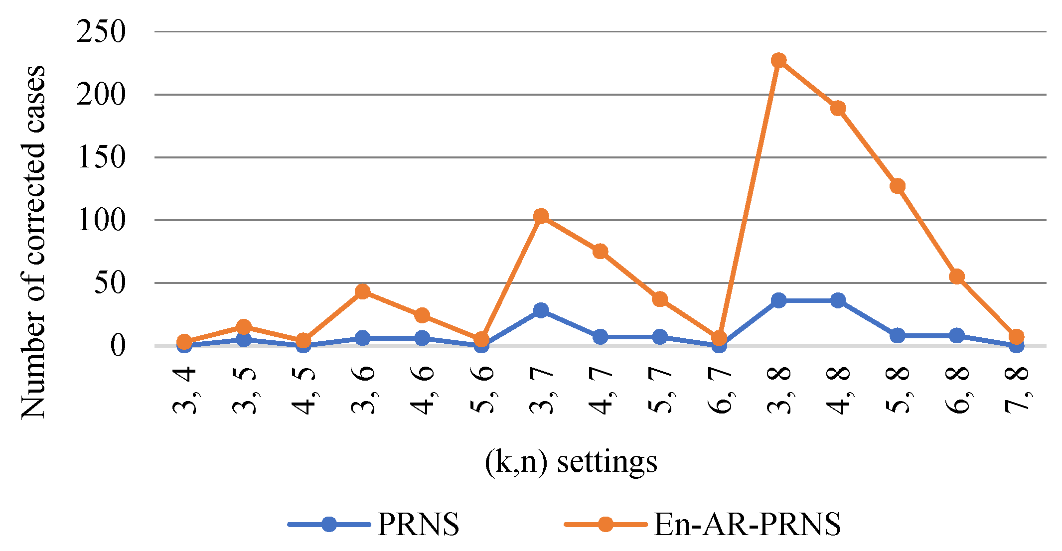
Figure 12 shows the number of recovery cases corrected by En-AR-PRNS and PRNS. We see that for $\left(3, 8\right)$ settings, the En-AR-PRNS corrected errors in 227 cases and PRNS in 36 cases.

Figure 12. Number of recovery cases corrected by En-AR-PRNS and PRNS.

Example 6 explains the results shown in Figure 12.

Example 6.

Let PRNS moduli 4-tuple be $m_1\left(x\right)=x^6+x+1$, $m_2\left(x\right)=x^6+x^3+1$, $m_3\left(x\right)=x^6+x^5+1$, and $m_4\left(x\right)=x^{12}+x^3+1$, where $k=3$, $r=1,$and $n=k+r=4$. The number of recovery cases found by PRNS is zero and by En-AR-PRNS it was three: $a_1\left(x\right)$, $a_2\left(x\right)$, and $a_3\left(x\right)$.

8. Discussion

The complexity of the presented algorithm motivates the usage of parallel computing. The inherent properties of PRNS attract much attention from both the scientific community and industry. Special interest is paid to the parallelization of the following algorithms:

• Coding: data conversion from conventional representation to PRNS;
• Decoding: data conversion from PRNS to conventional representation;
• Homomorphic computing: processing encrypted information without decryption;
• PRNS-based communication: transmitting shares;
• Computational intelligence: Estimating and classifying the security and reliability levels and finding adequate settings.

Coding. Since the computation of the residue for each modulo is independent, polynomial-to-PRNS conversion can be efficiently parallelized: independent calculation of residues $a_i\left(x\right)$; parallel calculation of each residue $a_i\left(x\right)$ based on a neural-like network approach to finite ring computations.

Decoding. Despite En-AR-PRNS performance improvement for PRNS-residues-to-polynomial conversion, presented in this paper, this conversion still significantly impacts the performance limitation of the whole system. It is one of the most difficult PRNS operations, and parallel computing can significantly improve it.

The following parallelization options are exploited:

• Parallel syndrome table search;
• Independent generation of the candidates, $V_P^l\left(x\right)$, with data recovery from all possible tuples of residues;
• Parallel calculation of ${{\displaystyle \sum }}_{i=1}^k{M}_i\left(x\right)·O_i\left(x\right)·a_i\left(x\right)$ and $R_A\left(x\right)·M\left(x\right)$ to generate the candidate $V_P^l\left(x\right)$;
• Independent calculation of the entropy, $H_W^l$, for each candidate. PRNS offers an important source of parallelism for addition, subtraction, and multiplication operations;
• Data are converted to many smaller polynomials (residues). Operations on initial data are substituted by faster operations on residuals executed in parallel. The complexity of operations is reduced;
• These features are used by the cryptography (RSA) community (Yen et al., 2003) [40], (Bajard and Imbert, 2004) [41], homomorphic encryption (Cheon et al., 2019) [42], and Microsoft SEAL (Laine, 2017) [43];
• Errors in a faulty computational logic element are localized in the corresponding residue without impacting other residues. This property is used in the algorithm for detecting errors in the AES cipher (Chu and Benaissa, 2013) [29] and control calculation results with encrypted data (Chervyakov et al., 2019) [2].
• Operations are based on fractional representations. Regardless of word sizes, they can be performed on bits without carrying in a single clock period. This improves computational efficiency, which has been proven to be especially useful in digital signal processing (Chang et al., 2015) [32], cryptography: RSA (Bajard and Imbert, 2004) [41], elliptic curve cryptography (Schinianakis et al., 2009 [44]; Guillermin, 2010) [45]), homomorphic encryption (Cheon et al., 2019 [42]; Laine, 2017 [43]), etc. This property is a way to approach a famous bound of speed at which addition and multiplication can be performed (Flynn, 2003) [46]. This bound, called Winograd’s bound, determines a minimum time for arithmetic operations and is an important basis for determining the comparative value of the various implementations of algorithms.

Other optimization criteria can also be considered, for instance, power consumption. Using small arithmetic units for the PRNS processor reduces the switching activities in each channel and dynamic power (Wang et al., 2000) [47]. The enhanced speed and low power consumption make the PRNS very encouraging in applications with intensive operations.

9. Conclusions

In this paper, we studied data reliability based on a polynomial residual number system and proposed a configurable, reliable, and secure distributed storage scheme, named En-AR-PRNS. We provided a theoretical analysis of the dynamic storage configurations.

Our main contributions were multi-fold:

• We proposed a novel decoding technique based on entropy to increase reliability. We showed that it can detect and correct more errors than the classical threshold-based PRNS;
• We provided a theoretical analysis of the reliability, redundancy, and coding/decoding speed, depending on configurable parameters to dynamically adapt the current configuration to various changes in the storage that are difficult to predict in advance;
• We reduced the computational complexity of the decoding from $O\left(D^2\right)$ down to $O\left(D·\log D\right)$using the concept of an approximation of the rank of a polynomial.

The main idea of adaptive optimization is to set $\left(k,n\right)$ PRNS parameters, moduli, and storages and dynamically change them to cope with different objective preferences and current properties. To this end, the past characteristics can be analyzed for a certain time interval to determine appropriate parameters. This interval should be set according to the dynamism of the characteristics and storage configurations.

This reactive approach deals with the uncertainty and non-stationarity associated with unauthorized data modifications, hardware and software malfunctions, disk errors, loss of data, malicious intrusions, denial of access for a long time, data transmission failures, etc. To detect changes, estimate, and classify the security and reliability levels, and violations of confidentiality, integrity, and availability, multi-objective techniques using computational intelligence and artificial intelligence can be applied. Future work will center on a comprehensive experimental study to assess the proposed mechanism’s efficiency and effectiveness in real dynamic systems under different types of errors and malicious attacks.

References

- Gomathisankaran, M.; Tyagi, A.; Namuduri, K. HORNS: A homomorphic encryption scheme for Cloud Computing using Residue Number System. In Proceedings of the 2011 45th Annual Conference on Information Sciences and Systems, Baltimore, MD, USA, 23–25 March 2011; pp. 1–5. [Google Scholar] [CrossRef]
- Chervyakov, N.; Babenko, M.; Tchernykh, A.; Kucherov, N.; Miranda-López, V.; Cortés-Mendoza, J.M. AR-RRNS: Configurable reliable distributed data storage systems for Internet of Things to ensure security. Futur. Gener. Comput. Syst. 2019, 92, 1080–1092. [Google Scholar] [CrossRef]
- Tchernykh, A.; Babenko, M.; Chervyakov, N.; Miranda-López, V.; Kuchukov, V.; Cortés-Mendoza, J.M.; Deryabin, M.; Kucherov, N.; Radchenko, G.; Avetisyan, A. AC-RRNS: Anti-collusion secured data sharing scheme for cloud storage. Int. J. Approx. Reason. 2018, 102, 60–73. [Google Scholar] [CrossRef]
- Tchernykh, A.; Schwiegelshohn, U.; Talbi, E.-G.; Babenko, M. Towards understanding uncertainty in cloud computing with risks of confidentiality, integrity, and availability. J. Comput. Sci. 2019, 36, 100581. [Google Scholar] [CrossRef]
- Tchernykh, A.; Babenko, M.; Chervyakov, N.; Miranda-Lopez, V.; Avetisyan, A.; Drozdov, A.Y.; Rivera-Rodriguez, R.; Radchenko, G.; Du, Z. Scalable Data Storage Design for Nonstationary IoT Environment with Adaptive Security and Reliability. IEEE Internet Things J. 2020, 7, 10171–10188. [Google Scholar] [CrossRef]
- Varghese, B.; Buyya, R. Next generation cloud computing: New trends and research directions. Future Gener. Comput. Syst. 2018, 79, 849–861. [Google Scholar] [CrossRef] [Green Version]
- Nachiappan, R.; Javadi, B.; Calheiros, R.N.; Matawie, K.M. Cloud storage reliability for Big Data applications: A state of the art survey. J. Netw. Comput. Appl. 2017, 97, 35–47. [Google Scholar] [CrossRef]
- Tan, C.B.; Hijazi, M.H.A.; Lim, Y.; Gani, A. A survey on Proof of Retrievability for cloud data integrity and availability: Cloud storage state-of-the-art, issues, solutions and future trends. J. Netw. Comput. Appl. 2018, 110, 75–86. [Google Scholar] [CrossRef]
- Sharma, Y.; Javadi, B.; Si, W. Sun, Reliability and energy efficiency in cloud computing systems: Survey and taxonomy. J. Netw. Comput. Appl. 2016, 74, 66–85. [Google Scholar] [CrossRef]
- Li, S.; Cao, Q.; Wan, S.; Qian, L.; Xie, C. HRSPC: A hybrid redundancy scheme via exploring computational locality to support fast recovery and high reliability in distributed storage systems. J. Netw. Comput. Appl. 2016, 66, 52–63. [Google Scholar] [CrossRef]
- Baker, T.; Mackay, M.; Shaheed, A.; Aldawsari, B. Security-Oriented Cloud Platform for SOA-Based SCADA. In Proceedings of the 2015 15th IEEE/ACM International Symposium on Cluster, Cloud and Grid Computing, Shenzhen, China, 4–7 May 2015; IEEE: Piscataway, NJ, USA, 2015; pp. 961–970. [Google Scholar] [CrossRef]
- Tchernykh, A.; Miranda-López, V.; Babenko, M.; Armenta-Cano, F.; Radchenko, G.; Drozdov, A.Y.; Avetisyan, A. Performance evaluation of secret sharing schemes with data recovery in secured and reliable heterogeneous multi-cloud storage. Clust. Comput. 2019, 22, 1173–1185. [Google Scholar] [CrossRef]
- Chen, X.; Qiming, H. The data protection of mapreduce using homomorphic encryption. In Proceedings of the 2013 IEEE 4th International Conference on Software Engineering and Service Science, Beijing, China, 23–25 May 2013; pp. 419–421. [Google Scholar] [CrossRef]
- Celesti, A.; Fazio, M.; Villari, M.; Puliafito, A. Adding long-term availability, obfuscation, and encryption to multi-cloud storage systems. J. Netw. Comput. Appl. 2016, 59, 208–218. [Google Scholar] [CrossRef]
- Tchernykh, A.; Babenko, M.; Kuchukov, V.; Miranda-Lopez, V.; Avetisyan, A.; Rivera-Rodriguez, R.; Radchenko, G. Data Reliability and Redundancy Optimization of a Secure Multi-cloud Storage Under Uncertainty of Errors and Falsifications. In Proceedings of the 2019 IEEE International Parallel and Distributed Processing Symposium Workshops (IPDPSW), Rio de Janeiro, Brazil, 20–24 May 2019; pp. 565–572. [Google Scholar] [CrossRef]
- Srisakthi, S.; Shanthi, A.P. Towards the Design of a Secure and Fault Tolerant Cloud Storage in a Multi-Cloud Environment. Inf. Secur. J. Glob. Perspect. 2015, 24, 109–117. [Google Scholar] [CrossRef]
- Hubbard, D.; Sutton, M. Top Threats to Cloud Computing V1.0, Cloud Security Alliance, 2010, (n.d.). Available online: https://ioactive.com/wp-content/uploads/2018/05/csathreats.v1.0-1.pdf. (accessed on 24 April 2021).
- Tchernykh, A.; Babenko, M.; Miranda-Lopez, V.; Drozdov, A.Y.; Avetisyan, A. WA-RRNS: Reliable Data Storage System Based on Multi-cloud. In Proceedings of the 2018 IEEE International Parallel and Distributed Processing Symposium Workshops (IPDPSW), Vancouver, BC, Canada, 21–25 May 2018; pp. 666–673. [Google Scholar] [CrossRef]
- Ghemawat, S.; Gobioff, H.; Leung, S.-T. The Google file system. ACM SIGOPS Oper. Syst. Rev. 2003, 37, 29. [Google Scholar] [CrossRef]
- Miranda-Lopez, V.; Tchernykh, A.; Babenko, M.; Avetisyan, A.; Toporkov, V.; Drozdov, A.Y. 2Lbp-RRNS: Two-Levels RRNS With Backpropagation for Increased Reliability and Privacy-Preserving of Secure Multi-Clouds Data Storage. IEEE Access 2020, 8, 199424–199439. [Google Scholar] [CrossRef]
- Lin, H.-Y.; Tzeng, W.-G. A Secure Erasure Code-Based Cloud Storage System with Secure Data Forwarding. IEEE Trans. Parallel Distrib. Syst. 2012, 23, 995–1003. [Google Scholar] [CrossRef]
- Dimakis, A.G.; Godfrey, P.B.; Wu, Y.; Wainwright, M.J.; Ramchandran, K. Network Coding for Distributed Storage Systems. IEEE Trans. Inf. Theory 2010, 56, 4539–4551. [Google Scholar] [CrossRef] [Green Version]
- Gentry, C. Computing arbitrary functions of encrypted data. Commun. ACM 2010, 53, 97. [Google Scholar] [CrossRef] [Green Version]
- Asmuth, C.; Bloom, J. A modular approach to key safeguarding. IEEE Trans. Inf. Theory 1983, 29, 208–210. [Google Scholar] [CrossRef]
- Mignotte, M. How to Share a Secret. In Cryptography. EUROCRYPT 1982; Lecture Notes in Computer Science; Beth, T., Ed.; Springer: Berlin/Heidelberg, Germany, 1982; Volume 149. [Google Scholar] [CrossRef]
- Lin, S.-J.; Chung, W.-H.; Han, Y.S. Novel Polynomial Basis and Its Application to Reed-Solomon Erasure Codes. In Proceedings of the 2014 IEEE 55th Annual Symposium on Foundations of Computer Science, Philadelphia, PA, USA, 18–21 October 2014; pp. 316–325. [Google Scholar] [CrossRef] [Green Version]
- Liu, J.; Huang, K.; Rong, H.; Wang, H.; Xian, M. Privacy-Preserving Public Auditing for Regenerating-Code-Based Cloud Storage. IEEE Trans. Inf. Forensics Secur. 2015, 10, 1513–1528. [Google Scholar] [CrossRef]
- Skavantzos, A.; Taylor, F.J. On the polynomial residue number system (digital signal processing). IEEE Trans. Signal Process. 1991, 39, 376–382. [Google Scholar] [CrossRef]
- Chu, J.; Benaissa, M. Error detecting AES using polynomial residue number systems. Microprocess. Microsyst. 2013, 37, 228–234. [Google Scholar] [CrossRef]
- Parker, M.G.; Benaissa, M. GF(pm) multiplication using polynomial residue number systems. IEEE Trans. Circuits Syst. II Analog. Digit. Signal Process 1995, 42, 718–721. [Google Scholar] [CrossRef]
- Chervyakov, N.I.; Babenko, M.G.; Kucherov, N.N. Development of Homomorphic Encryption Scheme Based on Polynomial Residue Number System. Sib. Electron. Math. Rep.-Sib. Elektron. Mat. Izv. 2015, 12, 33–41. [Google Scholar]
- Chang, C.-H.; Molahosseini, A.S.; Zarandi, A.A.E.; Tay, T.F. Residue Number Systems: A New Paradigm to Datapath Optimization for Low-Power and High-Performance Digital Signal Processing Applications. IEEE Circuits Syst. Mag. 2015, 15, 26–44. [Google Scholar] [CrossRef]
- Halbutogullari, A.; Koc, C.K. Parallel multiplication in GF(2k) using polynomial residue arithmetic. Des. Codes Cryptogr. 2000, 20, 155–173. [Google Scholar] [CrossRef]
- Geekbench Browser. Available online: https://browser.geekbench.com (accessed on 24 April 2021).
- Chervyakov, N.I.; Lyakhov, P.A.; Babenko, M.G.; Garyanina, A.I.; Lavrinenko, I.N.; Lavrinenko, A.V.; Deryabin, M.A. An efficient method of error correction in fault-tolerant modular neurocomputers. Neurocomputing 2016, 205, 32–44. [Google Scholar] [CrossRef]
- Kolmogorov, A.N. Three approaches to the definition of the concept “quantity of information”. Probl. Peredači Inf. 1965, 1, 3–11. [Google Scholar]
- Ivanov, M.; Sergiyenko, O.; Mercorelli, P.; Hernandez, W.; Tyrsa, V.; Hernandez-Balbuena, D.; Rodriguez Quinonez, J.C.; Kartashov, V.; Kolendovska, M.; Iryna, T. Effective informational entropy reduction in multi-robot systems based on real-time TVS. In Proceedings of the 2019 IEEE 28th International Symposium on Industrial Electronics (ISIE), Vancouver, BC, Canada, 12–14 June 2019; LNCS; Volume 11349, pp. 1162–1167. [Google Scholar] [CrossRef]
- Goh, V.T.; Siddiqi, M.U. Multiple error detection and correction based on redundant residue number systems. IEEE Trans. Commun. 2008, 56, 325–330. [Google Scholar] [CrossRef]
- Research and Compare Cloud Providers and Services. Available online: https://cloudharmony.com/status (accessed on 26 November 2021).
- Yen, S.-M.; Kim, S.; Lim, S.; Moon, S.-J. RSA speedup with chinese remainder theorem immune against hardware fault cryptanalysis. IEEE Trans. Comput. 2003, 52, 461–472. [Google Scholar] [CrossRef] [Green Version]
- Bajard, J.C.; Imbert, L. a full RNS implementation of RSA. IEEE Trans. Comput. 2004, 53, 769–774. [Google Scholar] [CrossRef]
- Cheon, J.H.; Han, K.; Kim, A.; Kim, M.; Song, Y. A Full RNS Variant of Approximate Homomorphic Encryption, in LNCS; Springer: Berlin/Heidelberg, Germany, 2019; Volume 11349, pp. 347–368. [Google Scholar] [CrossRef]
- Laine, K. Simple Encrypted Arithmetic Library 2.3.1., Microsoft Res. 2017. Available online: https://www.microsoft.com/en-us/research/uploads/prod/2017/11/sealmanual-2-3-1.pdf (accessed on 17 April 2021).
- Schinianakis, D.M.; Fournaris, A.P.; Michail, H.E.; Kakarountas, A.P.; Stouraitis, T. An RNS Implementation of an Fp Elliptic Curve Point Multiplier. IEEE Trans. Circuits Syst. I Regul. Pap. 2009, 56, 1202–1213. [Google Scholar] [CrossRef]
- Guillermin, N. A High Speed Coprocessor for Elliptic Curve Scalar Multiplications over Fp. In International Workshop on Cryptographic Hardware and Embedded Systems; Springer: Berlin/Heidelberg, Germany, 2010; pp. 48–64. [Google Scholar] [CrossRef]
- Flynn, M.J.; Oberman, S. Advanced Computer Arithmetic Design; Wiley: Hoboken, NJ, USA; p. 344.
- Wang, W.; Swamy, M.N.S.; Ahmad, M.O. An area-time-efficient residue-to-binary converter. In Proceedings of the 43rd IEEE Midwest Symposium on Circuits and Systems (Cat.No.CH37144), Lansing, MI, USA, 8–11 August 2000; Volume 2, pp. 904–907. [Google Scholar] [CrossRef]
Publisher’s Note: MDPI stays neutral with regard to jurisdictional claims in published maps and institutional affiliations. |
© 2021 by the authors. Licensee MDPI, Basel, Switzerland. This article is an open access article distributed under the terms and conditions of the Creative Commons Attribution (CC BY) license (https://creativecommons.org/licenses/by/4.0/).