A Fast Galerkin Approach for Solving the Fractional Rayleigh–Stokes Problem via Sixth-Kind Chebyshev Polynomials

Abstract

Herein, a spectral Galerkin method for solving the fractional Rayleigh–Stokes problem involving a nonlinear source term is analyzed. Two kinds of basis functions that are related to the shifted sixth-kind Chebyshev polynomials are selected and utilized in the numerical treatment of the problem. Some specific integer and fractional derivative formulas are used to introduce our proposed numerical algorithm. Moreover, the stability and convergence accuracy are derived in detail. As a final validation of our theoretical results, we present a few numerical examples.

1. Introduction

The importance of non-Newtonian fluids in science and industrial applications has piqued the interest of numerous researchers. There are many examples of non-Newtonian fluids such as in natural substances (lava, magma, gums, honey), in biology (semen, mucus, synovia, blood), in industry (molten polymer, lubricant, paint, ink, glue), in food products (ketchup, butter, mustard, chocolate, mayonnaise, cheese), and in cosmetics (cream, silicone, toothpaste, nail polish, soap solution). In this regard, the fractional Rayleigh–Stokes equation (FRSE) plays an important role in describing the dynamic behavior of some non-Newtonian fluids [1,2,3,4].

The nonlinear FRSE [5] is as follows:

$$u_t(x,t)-D_t^{\alpha }\left[a{u}_{xx}(x,t)\right]-b{u}_{xx}(x,t)=f(u(x,t),x,t),0<\alpha <1,$$

(1)

with, respectively, the following homogeneous initial and boundary conditions:

$$u(x,0)=0,0<x<\ell ,$$

and

$$u(0,t)=u(\ell ,t)=0,0<t\le \tau ,$$

where a and b are two positive constants and the nonlinear source term $f\left(u\right(x,t),x,t)$ satisfies the global Lipschitz condition with respect to $u(x,t)$. The symbol $D_t^{\alpha }$ is the Caputo fractional derivative operator of order $\alpha$ that describes the viscoelastic behavior of the flow. Some researchers have investigated and proposed a few methods for the solution of FRSE. In Ref. [6], the authors proposed the finite element method for the numerical solution of FRSE. In Ref. [7], the authors applied the radial basis function-generated finite difference method for the solution of the FRSE, while in [8], the authors solved the FRSE by using the spectral Jacobi–Galerkin method. Furthermore, an improved tau method for the multi-dimensional FRSE for a heated generalized second grade fluid was developed in [9]. Some other studies regarding the Rayleigh–Stokes problem can be found in [10,11].

Chebyshev polynomials (CPs) play significant roles in numerical analysis and approximation theory. There are well-known four kinds of CPs, which are specific types of Jacobi polynomials. These kinds of polynomials have been extensively used in a variety of papers related to numerical analysis; see, for instance, ref. [12,13,14]. The other two kinds of Chebyshev polynomials, namely, the fifth and sixth kinds of Chebyshev polynomials were investigated in [15]. These two classes are symmetric like the first and second kinds of Chebyshev polynomials. In fact, they are particular polynomials of the so-called “generalized ultraspherical polynomials” (see, for example, ref. [16,17]). Regrading these polynomials, their theoretical, as well as practical aspects, have attracted a significant attention from several authors. In this respect, Xu et al. [18] treated the fractional optimal control problems using sixth-kind Chebyshev wavelets. Moreover, Babaei et al. [19] employed Chebyshev polynomials of the sixth kind for solving the variable-order fractional nonlinear quadratic integro-differential equations. In addition, Jafari et al. [20] developed a spectral collocation method for treating the inverse reaction-diffusion–convection based on Chebyshev polynomials of the sixth kind. Some other contributions regarding sixth-kind Chebyshev polynomials can be found in [21,22], while for some contributions regarding Chebyshev polynomials of the fifth kind, one can referred to [23,24].

Since obtaining an exact solution is very computationally expensive for fractional differential equations, it is therefore impossible or extremely difficult to analytically solve such models. As a consequence, it has become an active research pursuit to analyze and implement high-efficient numerical techniques such as spectral methods for the simulation of solutions to these models. Spectral methods are based on the idea that approximate solutions to differential equations can be expressed as a series of truncated special functions. Three main spectral methods are employed, namely, the collocation, tau, and Galerkin methods. Readers interested in this subject can consult [25,26,27] for detailed explanations and applications of these techniques.

The following is a brief summary of the principal aims of this article:

• Construct and develop a new method for solving the nonlinear FRSE through shifted CPs of the sixth-kind by the application of the Galerkin method;
• Discuss the convergence and error analysis of the presented method;
• Present some numerical results to examine the applicability and accuracy of the algorithm.

The structure of the paper is as follows. Section 2 displays a few fundamental concepts related to Caputo fractional calculus. A few definitions and formulas concerning sixth-kind shifted CPs are also displayed. Section 3 discusses the Galerkin approach for the numerical treatment of the FRSE. The proposed double Chebyshev expansion is examined for convergence and error analysis in Section 4. Section 5 contains some numerical examples and comparisons between our numerical results and those produced by other approaches. A few conclusions are summarized in Section 6.

2. Preliminaries and Essential Relations

Essential definitions and formulas are included in this section.

2.1. Some Definitions and Properties of the Fractional Calculus

Definition 1

([28]). On the typical Lebesgue space $L_1[0,1]$, the Riemann–Liouville fractional integral operator of order ρ is defined as

$$I^{\rho }h\left(y\right)=\left\{\begin{array}{cc}{\displaystyle \frac{1}{\Gamma \left(\rho \right)}{\int }_0^y{(y-t)}^{\rho -1}h\left(t\right)dt,}\hfill & \rho >0,\hfill \\ h\left(y\right),\hfill & \rho =0.\hfill \end{array}\right.$$

Definition 2

([28]). The Caputo definition of the fractional-order derivative is:

$${\displaystyle D_y^{\rho }h\left(y\right)=\frac{1}{\Gamma (m-\rho )}{\int }_0^y{(y-t)}^{m-\rho -1}{h}^{\left(m\right)}\left(t\right)dt,\rho >0,y>0,}$$

where $m-1\le \rho <m,m\in \mathbb{N}$.

The operator $D_y^{\rho }$ fulfills the accompanying properties for $m-1\le \rho <m,m\in \mathbb{N},$

$$\begin{array}{cc}\hfill & \left(i\right)\left(D_y^{\rho }{I}^{\rho }h\right)\left(y\right)=h\left(y\right),\hfill \\ \hfill & \left(ii\right)\left(I^{\rho }{D}_y^{\rho }h\right)\left(y\right)=h\left(y\right)-\sum _{k=0}^{m-1}\frac{h^{\left(k\right)}\left(0^{+}\right)}{\Gamma (k+1)}{(y-a)}^k,y>0,\hfill \\ \hfill & \left(iii\right)D_y^{\rho }{y}^k=\frac{\Gamma (k+1)}{\Gamma (k+1-\rho )}{y}^{k-\rho },k\in \mathbb{N},k\ge \lceil \rho \rceil ,\hfill \end{array}$$

where $\lceil \rho \rceil$ is the smallest integer greater than or equal to $\rho$.

2.2. Some Basic Formulas and Properties of Sixth-Kind CPs and Their Shifted Ones

Sixth-kind Chebyshev polynomials $Y_i\left(t\right)$ [15] are orthogonal polynomials with respect to the weight function $\tilde{w}\left(t\right)=t^2\sqrt{1-t^2}$. The orthogonality relation of these polynomials is given by [21]

$$\underset{-1}{\overset{1}{\int }}{t}^2\sqrt{1-t^2}{Y}_i\left(t\right)Y_j\left(t\right)dt=\left\{\begin{array}{cc}{h}_i,\hfill & \mathrm{if} i=j,\hfill \\ 0,\hfill & \mathrm{if} i\ne j,\hfill \end{array}\right.$$

where

$$h_i=\frac{\pi }{2^{2i+3}}\left\{\begin{array}{cc}1,\hfill & \mathrm{if} i\mathrm{even},\hfill \\ \frac{i+3}{i+1},\hfill & \mathrm{if} i\mathrm{odd}.\hfill \end{array}\right.$$

These polynomials may be constructed using the following recursive formula:

$$\begin{array}{cc}\hfill & Y_i\left(t\right)=t{Y}_{i-1}\left(t\right)-\frac{i(i+1)+{(-1)}^i(2i+1)+1}{4i(i+1)}{Y}_{i-2}\left(t\right),Y_0\left(t\right)=1,Y_1\left(t\right)=t,i\ge 2.\hfill \end{array}$$

In [21], the authors also provide trigonometric representations of sixth-kind Chebyshev polynomials as follows:

$$\begin{array}{cc}\hfill & Y_{2i}(cos\theta )=\frac{sin(2i+2)\theta }{4^{i}sin\left(2\theta \right)},\hfill \\ & Y_{2i+1}(cos\theta )=\frac{2(i+2)cos\theta sin\left(\right(2i+3\left)\theta \right)-sin\left(\right(2i+4\left)\theta \right)}{4^{i+1}(i+1)sin\left(2\theta \right)cos\theta }.\hfill \end{array}$$

(2)

Now, we define the shifted orthogonal polynomials $Y_i^{*}\left(t\right)$ on $[0,\tau ]$ as:

$$Y_i^{*}\left(t\right)=Y_i\left(\frac{2t}{\tau }-1\right).$$

The following recurrence relation:

$$Y_i^{*}\left(t\right)=\left(\frac{2t}{\tau }-1\right)Y_{i-1}^{*}\left(t\right)-{\alpha }_i{Y}_{i-2}^{*}\left(t\right),Y_0^{*}\left(t\right)=1,Y_1^{*}\left(t\right)=\frac{2t}{\tau }-1,i\ge 2,$$

(3)

generates the sequence of the shifted sixth-kind CPs $Y_i^{*}\left(t\right)$ on $[0,\tau ]$, with

$${\alpha }_i=\frac{i(i+1)+{(-1)}^i(2i+1)+1}{4i(i+1)}.$$

These polynomials are orthogonal on $[0,\tau ]$ with respect to $\omega \left(t\right)={(2t-\tau )}^2\sqrt{t\tau -t^2}.$

More precisely, we have the following orthogonality relation (see, [21]):

$${\int }_0^{\tau }\omega \left(t\right)Y_i^{*}\left(t\right)Y_j^{*}\left(t\right)dt=h_{\tau ,i}{\delta }_{i,j},$$

(4)

where ${\delta }_{i,j}$ is the well-known Kronecker delta function and

$$h_{\tau ,i}=\frac{\pi {\tau }^4}{2^{2i+5}}\left\{\begin{array}{cc}1,\hfill & \mathrm{if} i\mathrm{even},\hfill \\ \frac{i+3}{i+1},\hfill & \mathrm{if} i\mathrm{odd}.\hfill \end{array}\right.$$

(5)

The power form representation of $Y_j^{*}\left(t\right)$ is given by [21]

$$Y_j^{*}\left(t\right)=\sum _{r=0}^j{B}_{r,j}{t}^r,$$

(6)

where

$${\displaystyle B_{r,j}=\frac{2^{2r-j}}{{\tau }^r(2r+1)!}\left\{\begin{array}{cc}{\displaystyle \sum _{k=\lfloor \frac{r+1}{2}\rfloor }^{\lfloor \frac{j}{2}\rfloor }\frac{{(-1)}^{\frac{j}{2}+k+r}(2k+r+1)!}{(2k-r)!},}\hfill & \mathrm{if}j\mathrm{even},\hfill \\ {\displaystyle \frac{2}{j+1}\sum _{k=\lfloor \frac{r}{2}\rfloor }^{\lfloor \frac{j-1}{2}\rfloor }\frac{{(-1)}^{\frac{j+1}{2}+k+r}(k+1)(2k+r+2)!}{(2k-r+1)!},}\hfill & \mathrm{if}j\mathrm{odd}.\hfill \end{array}\right.}$$

Another important formula of the $Y_j^{*}\left(t\right)$ is its inversion formula [21]

$$t^j=\sum _{i=0}^j{Q}_{i,j}{Y}_i^{*}\left(t\right),$$

where

$$Q_{i,j}=\frac{{\tau }^j(2j+1)!2^{i-2j+2}}{(j-i)!(i+j+4)!}\left\{\begin{array}{cc}(i+2)\left(i(i+4)+j^2+j+3\right),\hfill & \mathrm{if} i\mathrm{even},\hfill \\ (i+1)\left(i\right(i+4)+j(j+3)+6),\hfill & \mathrm{if}i\mathrm{odd}.\hfill \end{array}\right.$$

For more properties about $Y_j^{*}\left(t\right)$, see [21,22].

Theorem 1.

The first derivative of $Y_i^{*}\left(t\right)$ is given by [29]

$${\displaystyle \frac{d{Y}_i^{*}\left(t\right)}{dt}=\sum _{r=0}^{i-1}{M}_{r,i}{Y}_r^{*}\left(t\right),i\ge 1,}$$

and the coefficients $M_{r,i}$ are given by

$${\displaystyle M_{r,i}=\frac{2^{2-i+r}}{\tau }\left\{\begin{array}{cc}r+1,\hfill & i\mathit{even},r\mathit{odd},\hfill \\ {\displaystyle \frac{i(r+2)}{i+1},}\hfill & i\mathit{odd},\frac{i-r-1}{2}\mathit{even},\hfill \\ {\displaystyle \frac{(i+4)(r+2)}{i+1},}\hfill & i\mathit{odd},\frac{i-r-3}{2}\mathit{even},\hfill \\ 0,\hfill & \mathit{otherwise}.\hfill \end{array}\right.}$$

3. Galerkin Approach for Treating the FRSE

We begin by selecting our basis functions in this section. Then, using the spectral Galerkin approach, we present a numerical solution for solving the FRSE with homogeneous initial and boundary conditions.

3.1. Basis Functions Selection

The following are the basis functions that we choose:

$$\begin{array}{ccc}\hfill {\varphi }_i\left(t\right)& =& t{Y}_i^{*}\left(t\right),\hfill \\ \hfill {\psi }_i\left(x\right)& =& x(\ell -x)Y_i^{*}\left(x\right).\hfill \end{array}$$

(7)

The orthogonality relations of ${\varphi }_i\left(t\right)$ and ${\psi }_i\left(x\right)$ are respectively given by:

$${\int }_0^{\tau }\frac{{(2t-\tau )}^2\sqrt{t\tau -t^2}}{t^2}{\varphi }_i\left(t\right){\varphi }_j\left(t\right)dt=h_{\tau ,i}{\delta }_{i,j},$$

and

$${\int }_0^{\ell }\frac{{(2x-\ell )}^2}{x^{\frac{3}{2}}{(\ell -x)}^{\frac{3}{2}}}{\psi }_i\left(x\right){\psi }_j\left(x\right)dx=h_{\ell ,i}{\delta }_{i,j},$$

where $h_{\tau ,i}$ is as given in (13).

Theorem 2.

The second-order derivative of ${\psi }_i\left(x\right)$ can be written as [29]:

$${\displaystyle \frac{d^2{\psi }_i\left(x\right)}{d{x}^2}=\sum _{j=0}^i{\lambda }_{j,i}{Y}_j^{*}\left(x\right),}$$

where

$${\lambda }_{j,i}=\frac{1}{2^{i-j-1}}\left\{\begin{array}{cc}\frac{-(i+1)(i+2)}{2},\hfill & if i=j,\hfill \\ j+2,\hfill & if i,j\mathit{even}and\frac{i-j+2}{2}\mathit{odd},\hfill \\ -3(j+2),\hfill & if i,j\mathit{even}and\frac{i-j+2}{2}\mathit{even},\hfill \\ \frac{-(j+1)(i+2j+6)}{i+1},\hfill & if i,j\mathit{odd}and\frac{i-j+2}{2}\mathit{even},\hfill \\ \frac{(j+1)(-i+2j+2)}{i+1},\hfill & if i,j\mathit{odd}and\frac{i-j+2}{2}\mathit{odd},\hfill \\ 0,\hfill & \mathit{otherwise}.\hfill \end{array}\right.$$

Theorem 3.

The first-order derivative of ${\varphi }_i\left(t\right)$ is given by

$${\displaystyle \frac{d{\varphi }_i\left(t\right)}{dt}=\sum _{r=0}^i{A}_{r,i}{Y}_r^{*}\left(t\right),i\ge 1,}$$

where the coefficients $A_{r,i}$ are given by

$${\displaystyle A_{r,i}=\frac{\tau }{2}\left\{\begin{array}{cc}{M}_{r-1,i}+M_{r,i}+{\alpha }_{r+2}{M}_{r+1,i},\hfill & 1\le r\le i-2,\hfill \\ {\displaystyle \frac{2}{\tau }+M_{r-1,i},}\hfill & r=i,\hfill \\ M_{r,i}+M_{r-1,i},\hfill & r=i-1,\hfill \\ M_{0,i}+{\alpha }_2{M}_{1,i},\hfill & r=0.\hfill \end{array}\right.}$$

Theorem 4.

The following approximation formula holds for $0<\alpha <1$

$$D_t^{\alpha }{\varphi }_j\left(t\right)\approx \sum _{k=0}^N{\sigma }_{k,r,j,\alpha }{Y}_k^{*}\left(t\right),$$

where

$${\sigma }_{k,r,j,\alpha }=\sum _{r=0}^j\frac{(r+1)!B_{r,j}{\rho }_{k,r+1-\alpha }}{(r+1-\alpha )!}.$$

Remark 1.

The proofs of Theorems 3 and 4 are given in the Appendix A at the end of this paper.

3.2. Galerkin Solution for the FRSE

Now, consider the following two spaces:

$$\begin{array}{cc}\hfill & \Lambda =\mathrm{span}\{{\psi }_i\left(x\right){\varphi }_i\left(t\right):i,j=0,1\dots ,N\},\hfill \\ & \Delta =\left\{u\right(x,t)\in \Lambda :u(0,t)=u(\ell ,t)=u(x,0)=0,0<x<\ell ,0<t\le \tau \},\hfill \end{array}$$

then, any function $\tilde{u}(x,t)\in \Delta$ may be written as

$$\tilde{u}(x,t)=\sum _{i=0}^N\sum _{j=0}^N{c}_{ij}{\psi }_i\left(x\right){\varphi }_j\left(t\right).$$

Thanks to Theorems 2–4 along with the recurrence relation (3), we have the following expressions:

$$\begin{array}{cc}\hfill & {\tilde{u}}_t(x,t)=\frac{{\ell }^2}{4}\sum _{i=0}^N\sum _{j=0}^N\sum _{r=0}^j{A}_{r,j}{c}_{ij}[-Y_{i+2}^{*}\left(x\right)+\left(1-{\alpha }_{i+1}-{\alpha }_{i+2}\right)Y_i^{*}\left(x\right)-{\alpha }_i{\alpha }_{i+1}{Y}_{i-2}^{*}\left(x\right)]Y_r^{*}\left(t\right),\hfill \\ & {\displaystyle {\tilde{u}}_{xx}(x,t)=\frac{\tau }{2}\sum _{i=0}^N\sum _{j=0}^N\sum _{s=0}^i{\lambda }_{s,i}{c}_{ij}{Y}_s^{*}\left(x\right)\left[Y_{j+1}^{*}\left(t\right)+Y_j^{*}\left(t\right)+{\alpha }_{j+1}{Y}_{j-1}^{*}\left(t\right)\right],}\hfill \\ & {\displaystyle D_t^{\alpha }\left[{\tilde{u}}_{xx}(x,t)\right]\approx \frac{\tau }{2}\sum _{i=0}^N\sum _{j=0}^N\sum _{s=0}^i\sum _{k=0}^N{\lambda }_{s,i}{c}_{ij}{\sigma }_{k,r,j,\alpha }{Y}_s^{*}\left(x\right)Y_k^{*}\left(t\right).}\hfill \end{array}$$

Now, the residual of Equation (1) may be written in the following form:

$$\begin{array}{cc}\hfill \mathbb{R}(x,t)& ={\tilde{u}}_t(x,t)-D_t^{\alpha }\left[a{\tilde{u}}_{xx}(x,t)\right]-b{\tilde{u}}_{xx}(x,t)-f(\tilde{u}(x,t),x,t)\hfill \\ & =\frac{{\ell }^2}{4}\sum _{i=0}^N\sum _{j=0}^N\sum _{r=0}^j{A}_{r,j}{c}_{ij}[-Y_{i+2}^{*}\left(x\right)+\left(1-{\alpha }_{i+1}-{\alpha }_{i+2}\right)Y_i^{*}\left(x\right)-{\alpha }_i{\alpha }_{i+1}{Y}_{i-2}^{*}\left(x\right)]Y_r^{*}\left(t\right)\hfill \\ & {\displaystyle -\frac{b\tau }{2}\sum _{i=0}^N\sum _{j=0}^N\sum _{s=0}^i{\lambda }_{s,i}{c}_{ij}{Y}_s^{*}\left(x\right)\left[Y_{j+1}^{*}\left(t\right)+Y_j^{*}\left(t\right)+{\alpha }_{j+1}{Y}_{j-1}^{*}\left(t\right)\right]}\hfill \\ & -\frac{a\tau }{2}\sum _{i=0}^N\sum _{j=0}^N\sum _{s=0}^i\sum _{k=0}^N{\lambda }_{s,i}{c}_{ij}{\sigma }_{k,r,j,\alpha }{Y}_s^{*}\left(x\right)Y_k^{*}\left(t\right)-f(\tilde{u}(x,t),x,t).\hfill \end{array}$$

(8)

The following system of equations can be obtained using the Galerkin method as follows:

$${\int }_0^{\tau }{\int }_0^{\ell }\mathbb{R}(x,t){\psi }_m\left(x\right){\varphi }_n\left(t\right)w(x,t)dxdt=0,0\le m,n\le N,$$

(9)

where $w(x,t)=\frac{{(2x-\ell )}^2{(2t-\tau )}^2\sqrt{t\tau -t^2}}{t\sqrt{x(\ell -x)}}.$

By virtue of Equation (8), we can rewrite Equation (9) as

$$\begin{array}{cc}\hfill & \frac{{\ell }^2}{4}\sum _{i=0}^N\sum _{j=0}^N\sum _{r=0}^j{A}_{r,j}{c}_{ij}[-h_{\ell ,i+2}{\delta }_{i+2,m}+\left(1-{\alpha }_{i+1}-{\alpha }_{i+2}\right)h_{\ell ,i}{\delta }_{i,m}-{\alpha }_i{\alpha }_{i+1}{h}_{\ell ,i-2}{\delta }_{i-2,m}]{\delta }_{r,n}{h}_{\tau ,r}\hfill \\ & {\displaystyle -\frac{b\tau }{2}\sum _{i=0}^N\sum _{j=0}^N\sum _{s=0}^i{\lambda }_{s,i}{c}_{ij}{\delta }_{s,m}{h}_{\ell ,s}\left[h_{\tau ,j+1}{\delta }_{j+1,n}+h_{\tau ,j}{\delta }_{j,n}+{\alpha }_{j+1}{h}_{\tau ,j-1}{\delta }_{j-1,n}\right]}\hfill \\ & -\frac{a\tau }{2}\sum _{i=0}^N\sum _{j=0}^N\sum _{s=0}^i{\lambda }_{s,i}{c}_{ij}{\sigma }_{n,r,j,\alpha }{\delta }_{s,m}{h}_{\ell ,s}{h}_{\tau ,n}-{\overline{f}}_{m,n}=0,0\le m,n\le N,\hfill \end{array}$$

(10)

where

$${\overline{f}}_{m,n}={\int }_0^{\tau }{\int }_0^{\ell }f(\tilde{u}(x,t),x,t){\psi }_m\left(x\right){\varphi }_n\left(t\right)w(x,t)dxdt.$$

Equation (10) constructs a system of non-linear algebraic equations with unknown expansion coefficients $c_{ij}$ of dimension ${(N+1)}^2$, which can be solved using the well-known Newton’s iterative approach with zero initial approximations, and thus an approximation of the solution can be obtained.

3.3. Transformation to the Homogeneous Initial and Boundary Conditions

By virtue of the following transformation:

$$u(x,t):=v(x,t)+\overline{v}(x,t),$$

where

$$\overline{v}(x,t)=\left(1-\frac{x}{\ell }\right)\left(u(0,t)-u(0,0)\right)+\frac{x}{\ell }\left(u(\ell ,t)-u(\ell ,0)\right)+u(x,0).$$

the FRSE (1) with non-homogeneous initial and boundary conditions can be transformed into the following form:

$$v_t(x,t)-D_t^{\alpha }\left[a{v}_{xx}(x,t)\right]-b{v}_{xx}(x,t)=\widehat{f}(v(x,t),x,t),0<\alpha <1,$$

with homogeneous initial and boundary conditions

$$\begin{array}{cc}\hfill & v(x,0)=0,0<x<\ell ,\hfill \\ & v(0,t)=v(\ell ,t)=0,0<t\le \tau ,\hfill \end{array}$$

where

$$\widehat{f}(v(x,t),x,t)=f(u(x,t),x,t)-{\overline{v}}_t(x,t)+D_t^{\alpha }\left[a{\overline{v}}_{xx}(x,t)\right]+b{\overline{v}}_{xx}(x,t).$$

4. Convergence Analysis

We present an upper estimate for the truncation error as well as the stability of the proposed approximate solution in this section.

Theorem 5.

Consider the function: $u(x,t)={\gamma }_1\left(x\right){\gamma }_2\left(t\right)\in L_{w(x,t)}^2$, with ${\gamma }_1\left(x\right)$ and ${\gamma }_2\left(t\right)$ having bounded third derivatives that satisfy the expansion:

$$u(x,t)=\sum _{i=0}^{\infty }\sum _{j=0}^{\infty }{c}_{ij}{\psi }_i\left(x\right){\varphi }_j\left(t\right).$$

(11)

Then, the above series (11) is uniformly convergent to $u(x,t)$ and the expansion coefficients $c_{ij}$ satisfy the inequality:

$$|c_{ij}|⪅\frac{1}{i^3{j}^3},\forall i,j>3,$$

(12)

where ⪅ means that a generic constant d exists such that $|c_{ij}|\le \frac{d}{i^3{j}^3}.$

Proof. 

The orthogonality relations of ${\psi }_i\left(x\right)$ and ${\varphi }_j\left(t\right)$ enable one to write

$$c_{ij}=\frac{1}{h_{\ell ,i}{h}_{\tau ,j}}{\int }_0^{\tau }{\int }_0^{\ell }u(x,t){\psi }_i\left(x\right){\varphi }_j\left(t\right)w(x,t)dxdt.$$

By the hypotheses of the theorem, we obtain

$$c_{ij}=\frac{1}{h_{\ell ,i}{h}_{\tau ,j}}\left({\int }_0^{\ell }{(2x-\ell )}^2\sqrt{x\ell -x^2}{\gamma }_1\left(x\right)Y_i^{*}\left(x\right)dx\right)\left({\int }_0^{\tau }{(2t-\tau )}^2\sqrt{t\tau -t^2}{\gamma }_2\left(t\right)Y_j^{*}\left(t\right)dt\right).$$

By virtue of the two substitutions:

$$x=\frac{\ell }{2}(1+cos{\theta }_1),t=\frac{\tau }{2}(1+cos{\theta }_2),$$

the last equation turns into the form

$$\begin{array}{cc}\hfill c_{ij}& =\frac{1}{4h_i}{\int }_0^{\pi }{\gamma }_1\left(\frac{\ell }{2}(1+cos{\theta }_1)\right)Y_i(cos{\theta }_1){sin}^2\left(2{\theta }_1\right)d{\theta }_1\hfill \\ & \times \frac{1}{4h_j}{\int }_0^{\pi }{\gamma }_2\left(\frac{\tau }{2}(1+cos{\theta }_2)\right)Y_j(cos{\theta }_2){sin}^2\left(2{\theta }_2\right)d{\theta }_2.\hfill \end{array}$$

(13)

Now, we have four cases:

(i)

If $i,j\mathrm{are}\mathrm{even}$

Integrating Equation (13) by parts three times as followed in Theorem 5 in [21] and making use of the trigonometric representations (2) leads to the following estimation:

$$|c_{ij}|⪅\frac{1}{i^3{j}^3},\forall i,j>3.$$

We can also deduce the following estimations in the following cases

(ii)

If $i,j\mathrm{are}\mathrm{odd}$

$$|c_{ij}|⪅\frac{1}{i^3{j}^3},\forall i,j>3.$$

(iii)

If $i\mathrm{is}\mathrm{even};j\mathrm{is}\mathrm{odd}$

$$|c_{ij}|⪅\frac{1}{i^3{j}^3},\forall i,j>3.$$

(iv)

If $i\mathrm{is}\mathrm{odd};j\mathrm{is}\mathrm{even}$

$$|c_{ij}|⪅\frac{1}{i^3{j}^3},\forall i,j>3.$$

This completes the proof of Theorem 5. □

Theorem 6.

If $u(x,t)$ satisfies the hypothesis of Theorem 5 and if ${\displaystyle u_N(x,t)=\sum _{i=0}^N\sum _{j=0}^N{c}_{ij}{\psi }_i\left(x\right){\varphi }_j\left(t\right)}$, then the following estimate of truncation error is fulfilled:

$${\parallel u(x,t)-u_N(x,t)\parallel }_{L_{w(x,t)}^2}⪅N^{\frac{-3}{2}}.$$

Proof. 

From the definition of $u(x,t)$ and $u_N(x,t),$ we obtain

$$\begin{array}{cc}\hfill & {\parallel u(x,t)-u_N(x,t)\parallel }_{L_{w(x,t)}^2}\hfill \\ \hfill & \le {∥\sum _{i=0}^N\sum _{j=N+1}^{\infty }{c}_{ij}{\psi }_i\left(x\right){\varphi }_j\left(t\right)∥}_{L_{w(x,t)}^2}+{∥\sum _{i=N+1}^{\infty }\sum _{j=0}^{\infty }{c}_{ij}{\psi }_i\left(x\right){\varphi }_j\left(t\right)∥}_{L_{w(x,t)}^2}\hfill \\ & =\sum _{i=0}^N\sum _{j=N+1}^{\infty }|c_{ij}|\sqrt{(1-{\alpha }_{i+1}-{\alpha }_{i+2})h_{\ell ,i}{h}_{\tau ,j}}+\sum _{i=N+1}^{\infty }\sum _{j=0}^{\infty }|c_{ij}|\sqrt{(1-{\alpha }_{i+1}-{\alpha }_{i+2})h_{\ell ,i}{h}_{\tau ,j}}\hfill \\ & =\sum _{j=N+1}^{\infty }\left(|c_{0j}|b_0+|c_{1j}|b_1+|c_{2j}|b_2+|c_{3j}|b_3\right)\sqrt{h_{\tau ,j}}\hfill \\ & +\sum _{i=4}^N\sum _{j=N+1}^{\infty }|c_{ij}|\sqrt{(1-{\alpha }_{i+1}-{\alpha }_{i+2})h_{\ell ,i}{h}_{\tau ,j}}\hfill \\ & +\sum _{i=N+1}^{\infty }\left(|c_{i0}|b_4+|c_{i1}|b_5+|c_{i2}|b_6+|c_{i3}|b_7\right)\sqrt{(1-{\alpha }_{i+1}-{\alpha }_{i+2})h_{\ell ,i}}\hfill \\ & +\sum _{i=N+1}^{\infty }\sum _{j=4}^{\infty }|c_{ij}|\sqrt{(1-{\alpha }_{i+1}-{\alpha }_{i+2})h_{\ell ,i}{h}_{\tau ,j}},\hfill \end{array}$$

(14)

where

$$b_r=\left\{\begin{array}{cc}\sqrt{(1-{\alpha }_{r+1}-{\alpha }_{r+2})h_{\ell ,r}},\hfill & \mathrm{if} r=0,1,2,3,\hfill \\ \sqrt{h_{\tau ,r}},\hfill & \mathrm{if} r=4,5,6,7.\hfill \end{array}\right.$$

Now, following steps similar to those given in Theorem 5, we obtain

$$|c_{0j}|⪅\frac{1}{j^3},|c_{1j}|⪅\frac{1}{j^3},|c_{2j}|⪅\frac{1}{j^3},|c_{3j}|⪅\frac{1}{j^3},\forall j>3,$$

(15)

and

$$|c_{i0}|⪅\frac{1}{i^3},|c_{i1}|⪅\frac{1}{i^3},|c_{i2}|⪅\frac{1}{i^3},|c_{i3}|⪅\frac{1}{i^3},\forall i>3.$$

(16)

Inserting Equations (12), (15) and (16) into Equation (14) and using

$$\sqrt{(1-{\alpha }_{i+1}-{\alpha }_{i+2})}<1,i\ge 0,and|h_{\ell ,j}|⪅\frac{1}{2^{2j}},j\ge 0,$$

(17)

we obtain

$$\begin{array}{cc}\hfill {\parallel u(x,t)-u_N(x,t)\parallel }_{L_{w(x,t)}^2}& \le \sum _{j=N+1}^{\infty }\frac{{\widehat{b}}_0}{j^3{2}^j}+\sum _{i=4}^N\sum _{j=N+1}^{\infty }\frac{{\widehat{b}}_1}{i^3{j}^3{2}^{i+j}}+\sum _{i=N+1}^{\infty }\frac{{\widehat{b}}_2}{i^3{2}^i}\hfill \\ & +\sum _{i=N+1}^{\infty }\sum _{j=4}^{\infty }\frac{{\widehat{b}}_3}{i^3{j}^3{2}^{i+j}},\hfill \end{array}$$

where ${\widehat{b}}_r,r=0,1,2,3$ are constants.

However, for all $j>0,$ we have $\frac{1}{j^3{2}^j}<\frac{1}{j^{\frac{5}{2}}};$ thus

$$\begin{array}{cc}\hfill {\parallel u(x,t)-u_N(x,t)\parallel }_{L_{w(x,t)}^2}& \le \sum _{j=N+1}^{\infty }\frac{{\widehat{b}}_0}{j^{\frac{5}{2}}}+\sum _{i=4}^N\sum _{j=N+1}^{\infty }\frac{{\widehat{b}}_1}{i^{\frac{5}{2}}{j}^{\frac{5}{2}}}+\sum _{i=N+1}^{\infty }\frac{{\widehat{b}}_2}{i^{\frac{5}{2}}}\hfill \\ & +\sum _{i=N+1}^{\infty }\sum _{j=4}^{\infty }\frac{{\widehat{b}}_3}{i^{\frac{5}{2}}{j}^{\frac{5}{2}}}.\hfill \end{array}$$

(18)

and hence, the application of the integral test [30] enables us to write Equation (18) as

$${\parallel u(x,t)-u_N(x,t)\parallel }_{L_{w(x,t)}^2}⪅N^{\frac{-3}{2}}.$$

□

Theorem 7.

Under the assumptions of Theorem 5, we have

$${\parallel u_{N+1}(x,t)-u_N(x,t)\parallel }_{L_{w(x,t)}^2}⪅2^{-N}.$$

Proof. 

We have

$$\begin{array}{cc}\hfill {\parallel u_{N+1}(x,t)-u_N(x,t)\parallel }_{L_{w(x,t)}^2}& ={∥{\displaystyle \sum _{i=0}^N{c}_{i,N+1}{\psi }_i\left(x\right){\varphi }_{N+1}\left(t\right)+\sum _{j=0}^{N+1}{c}_{N+1,j}{\psi }_{N+1}\left(x\right){\varphi }_j\left(t\right)}∥}_{L_{w(x,t)}^2}\hfill \\ & \le {∥{\displaystyle \sum _{i=0}^N{c}_{i,N+1}{\psi }_i\left(x\right){\varphi }_{N+1}\left(t\right))}∥}_{L_{w(x,t)}^2}+{∥{\displaystyle \sum _{j=0}^{N+1}{c}_{N+1,j}{\psi }_{N+1}\left(x\right){\varphi }_j\left(t\right)}∥}_{L_{w(x,t)}^2}\hfill \\ & {\displaystyle <\sum _{i=0}^N|c_{i,N+1}|\sqrt{h_{\ell ,i}{h}_{\tau ,N+1}}+\sum _{j=0}^{N+1}|c_{N+1,j}|\sqrt{h_{\ell ,N+1}{h}_{\tau ,j}}}\hfill \\ & =\sqrt{h_{\tau ,N+1}}\left(|c_{0,N+1}|\sqrt{h_{\ell ,0}}+|c_{1,N+1}|\sqrt{h_{\ell ,1}}+|c_{2,N+1}|\sqrt{h_{\ell ,2}}+|c_{3,N+1}|\sqrt{h_{\ell ,3}}\right)\hfill \\ & +\sqrt{h_{\ell ,N+1}}\left(|c_{N+1,0}|\sqrt{h_{\tau ,0}}+|c_{N+1,1}|\sqrt{h_{\tau ,1}}+|c_{N+1,2}|\sqrt{h_{\tau ,2}}+|c_{N+1,3}|\sqrt{h_{\tau ,3}}\right)\hfill \\ & +\sqrt{h_{\tau ,N+1}}\sum _{i=4}^N|c_{i,N+1}|\sqrt{h_{\ell ,i}}+\sqrt{h_{\ell ,N+1}}\sum _{j=4}^{N+1}|c_{N+1,j}|\sqrt{h_{\tau ,j}}.\hfill \end{array}$$

(19)

Based on Equations (15)–(17) and Theorem 5 we obtain

$$\begin{array}{cc}\hfill & |c_{0,N+1}|⪅\frac{1}{N^3},|c_{1,N+1}|⪅\frac{1}{N^3},|c_{2,N+1}|⪅\frac{1}{N^3},|c_{3,N+1}|⪅\frac{1}{N^3},\hfill \\ & |c_{N+1,0}|⪅\frac{1}{N^3},|c_{N+1,1}|⪅\frac{1}{N^3},|c_{N+1,2}|⪅\frac{1}{N^3},|c_{N+1,3}|⪅\frac{1}{N^3},\hfill \\ & |h_{\ell ,j}|⪅\frac{1}{2^{2j}},|h_{\ell ,N+1}|⪅\frac{1}{2^{2N}},|h_{\tau ,j}|⪅\frac{1}{2^{2j}},|h_{\tau ,N+1}|⪅\frac{1}{2^{2N}},\hfill \\ & |c_{i,N+1}|⪅\frac{1}{i^3{N}^3},|c_{N+1,i}|⪅\frac{1}{i^3{N}^3}.\hfill \end{array}$$

(20)

Now, inserting Equation (20) into Equation (19) and using the inequality: $\frac{1}{j^3{2}^j}\le \frac{1}{2^j},$$\forall j>0,$ along with the following approximation

$$\sum _{i=a+1}^{b}f\left(i\right)\le {\int }_{x=a}^{b}f\left(x\right)dx,$$

where f is decreasing function, the desired result can be obtained. □

5. Illustrative Examples

In this section, the technique presented in Section 3 is applied to solve the nonlinear FRSE. Three illustrative examples are used to demonstrate the effectiveness and applicability of the proposed technique.

Example 1.

Consider the FRSE of the form

$$u_t(x,t)-D_t^{\alpha }\left[u_{xx}(x,t)\right]-u_{xx}(x,t)=f(u(x,t),x,t),0<\alpha <1,$$

where

$$\begin{array}{cc}\hfill f\left(u\right(x,t),x,t)=& sin\left(u\right)+2tx(x-\ell )\left[\left(5x^2-5x\ell +{\ell }^2\right)\left(\frac{6}{\Gamma (3-\alpha )}{t}^{1-\alpha }+3t\right)-x^2{(x-\ell )}^2\right]\hfill \\ & -sin\left(x^3{(\ell -x)}^3{t}^2\right),\hfill \end{array}$$

along with the following initial and boundary conditions:

$$\begin{array}{cc}\hfill & u(x,0)=0,0<x<\ell ,\hfill \\ & u(0,t)=0,u(\ell ,t)=0,0<t\le \tau .\hfill \end{array}$$

The exact solution of this problem is $u(x,t)=x^3{(\ell -x)}^3{t}^2.$

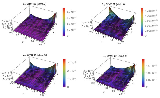
In Table 1, we reported the computational time (CPU time) and compared the $L_2$ errors of the present method with method in [5] at $\ell =\tau =1$. We see in this table that the results are accurate for small choices of N. Table 2 lists the $L_{\infty }$ errors for different values of α at $N=6$ when $\ell =2$ and $\tau =3$ and the CPU time. Figure 1 illustrates the $L_{\infty }$ error for $\alpha =0.3$ (left) and $\alpha =0.7$ (right) at $N=4$ when $\ell =5$ and $\tau =10$. We can see from Table 1 and Table 2 and Figure 1 that the proposed method is appropriate and effective. This demonstrates the advantage of our method compared to some other numerical methods.

Table 1. The $L_2$ errors for Example 1.

	Method in [5]		Presented Method
$\mathit{\alpha }$	h = $\frac{1}{5000},$ T = $\frac{1}{128}$	T = $\frac{1}{5000},$ h = $\frac{1}{128}$	$\mathit{N}=6$	CPU Time
0.1	$1.1552\times {10}^{-6}$	$1.4408\times {10}^{-6}$	$8.5446\times {10}^{-16}$	35.703
0.5	$1.0805\times {10}^{-6}$	$1.4007\times {10}^{-6}$	$3.0349\times {10}^{-15}$	36.109
0.9	$8.1511\times {10}^{-7}$	$1.3682\times {10}^{-6}$	$7.5113\times {10}^{-16}$	38.594

Table 2. The $L_{\infty }$ errors for Example 1.

$\mathit{\alpha }$	0.1	0.5	0.9
$L_{\infty }$ error	5.12335 $\times {10}^{-13}$	7.70939 $\times {10}^{-13}$	9.18376 $\times {10}^{-13}$
CPU time	46.029	43.813	44.406

Figure 1. The $L_{\infty }$ error for Example 1.

Example 2.

Consider the FRSE of the form

$$u_t(x,t)-D_t^{\alpha }\left[u_{xx}(x,t)\right]-u_{xx}(x,t)=f(u(x,t),x,t),0<\alpha <1,$$

where

$$f(u(x,t),x,t)=u^2+sin\left(\pi x\right)\left[\frac{2{\pi }^2}{\Gamma (3-\alpha )}{t}^{2-\alpha }+{\pi }^2{t}^2+2t\right]-t^4{sin}^2\left(\pi x\right),$$

along with the following initial and boundary conditions:

$$\begin{array}{cc}\hfill & u(x,0)=0,0<x<\ell ,\hfill \\ & u(0,t)=0,u(\ell ,t)=0,0<t\le \tau .\hfill \end{array}$$

The exact solution of this problem is $u(x,t)=t^{2}sin\left(\pi x\right).$

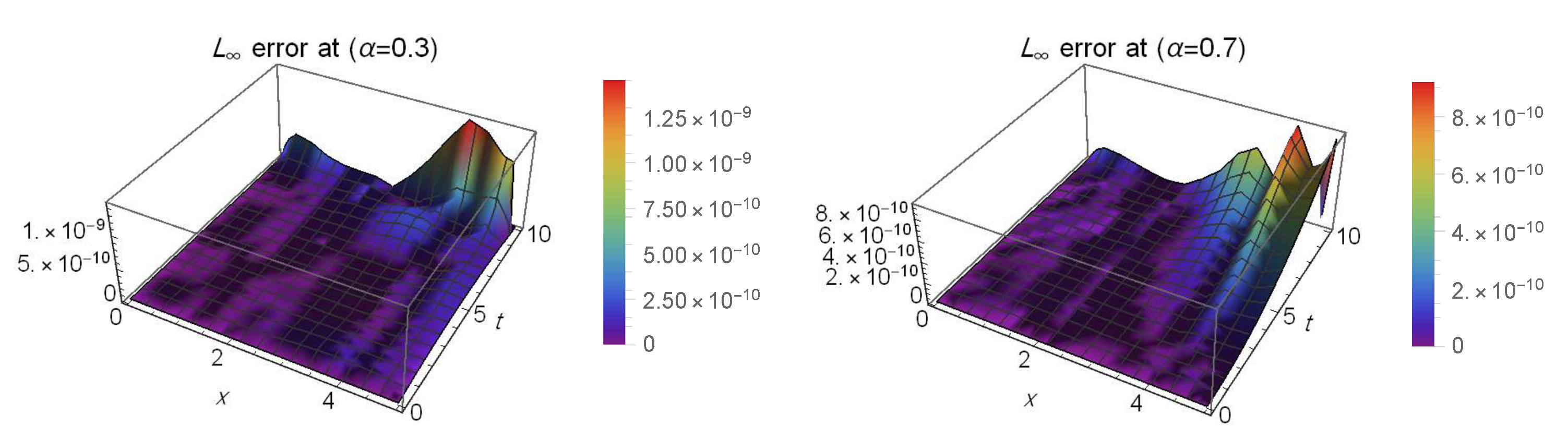
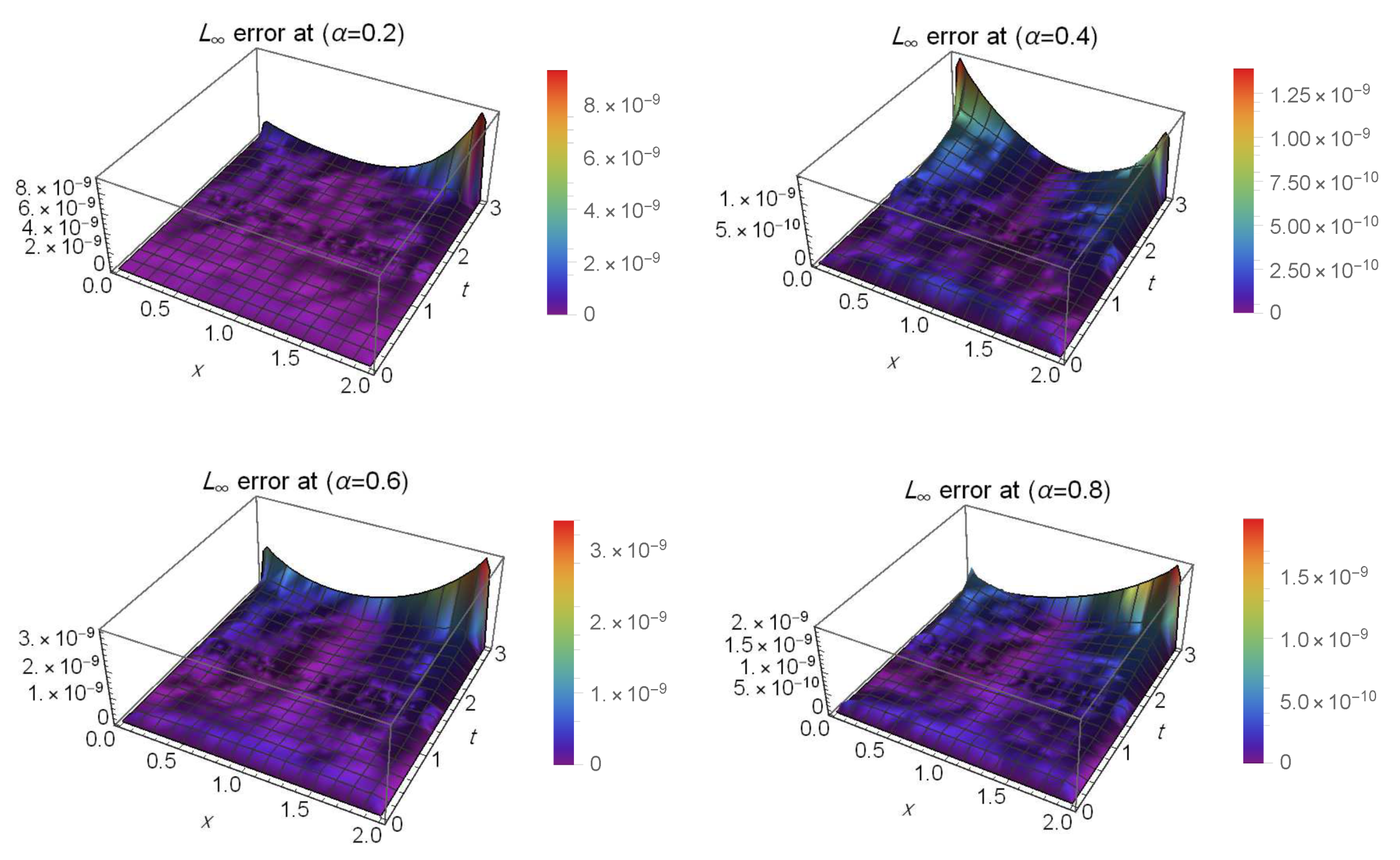
Table 3 presents the CPU time and a comparison of the $L_2$ errors between our proposed method and the method in [5] at $\ell =\tau =1$. It can be found that the obtained results of the presented method are more accurate than the method in [5]. Moreover, Figure 2 sketches the $L_{\infty }$ error for different values of α at $N=16$ when $\ell =2$ and $\tau =3$. This figure show that the numerical and exact solutions are almost identical. In Table 4. we list the absolute error for $\alpha =0.5$ at $N=18$ when $\ell =5$ and $\tau =10$. As can be seen, the proposed method presents better accuracy.

Table 3. The $L_2$ errors for Example 2.

	Method in [5]		Presented Method
$\mathit{\alpha }$	h = $\frac{1}{5000},$ T = $\frac{1}{128}$	T = $\frac{1}{5000},$ h = $\frac{1}{128}$	$\mathit{N}=12$	CPU Time
0.1	$9.1909\times {10}^{-5}$	$5.1027\times {10}^{-5}$	$2.53148\times {10}^{-12}$	94.218
0.5	$8.4317\times {10}^{-5}$	$4.4651\times {10}^{-5}$	$1.25044\times {10}^{-12}$	95.718
0.9	$6.2864\times {10}^{-5}$	$4.0543\times {10}^{-5}$	$8.47489\times {10}^{-13}$	94.78

Figure 2. The $L_{\infty }$ error for Example 2.

Table 4. The absolute errors for Example 2.

x	Absolute Error ($\mathit{t}=3$)	Absolute Error ($\mathit{t}=6$)	Absolute Error ($\mathit{t}=9$)
0.5	0.000459395	0.00202554	0.00477932
1	0.000348895	0.00169837	0.00419428
1.5	0.000275978	0.00147336	0.00378444
2	0.000234718	0.00134231	0.00352795
2.5	0.000221372	0.00129796	0.00323485
3	0.000234709	0.00133006	0.00170189
3.5	0.000275919	0.00139784	0.00634153
4	0.000348564	0.00126173	0.05467222
4.5	0.000457683	0.00007223	0.21660543

Example 3.

Consider the FRSE of the form

$$u_t(x,t)-D_t^{\alpha }\left[u_{xx}(x,t)\right]-u_{xx}(x,t)=f(u(x,t),x,t),0<\alpha <1,$$

where

$$f(u(x,t),x,t)=u^2+e^x\left((3-\alpha )t^{2-\alpha }-\frac{\Gamma (4-\alpha )}{\Gamma (4-2\alpha )}{t}^{3-2\alpha }-t^{3-\alpha }\right)-e^{2x}{t}^{6-2\alpha },$$

along with the following initial and boundary conditions:

$$\begin{array}{cc}\hfill & u(x,0)=0,0<x<1,\hfill \\ & u(0,t)=t^{3-\alpha },u(1,t)=e{t}^{3-\alpha },0<t\le 1.\hfill \end{array}$$

The exact solution of this problem is $u(x,t)=e^x{t}^{3-\alpha }.$

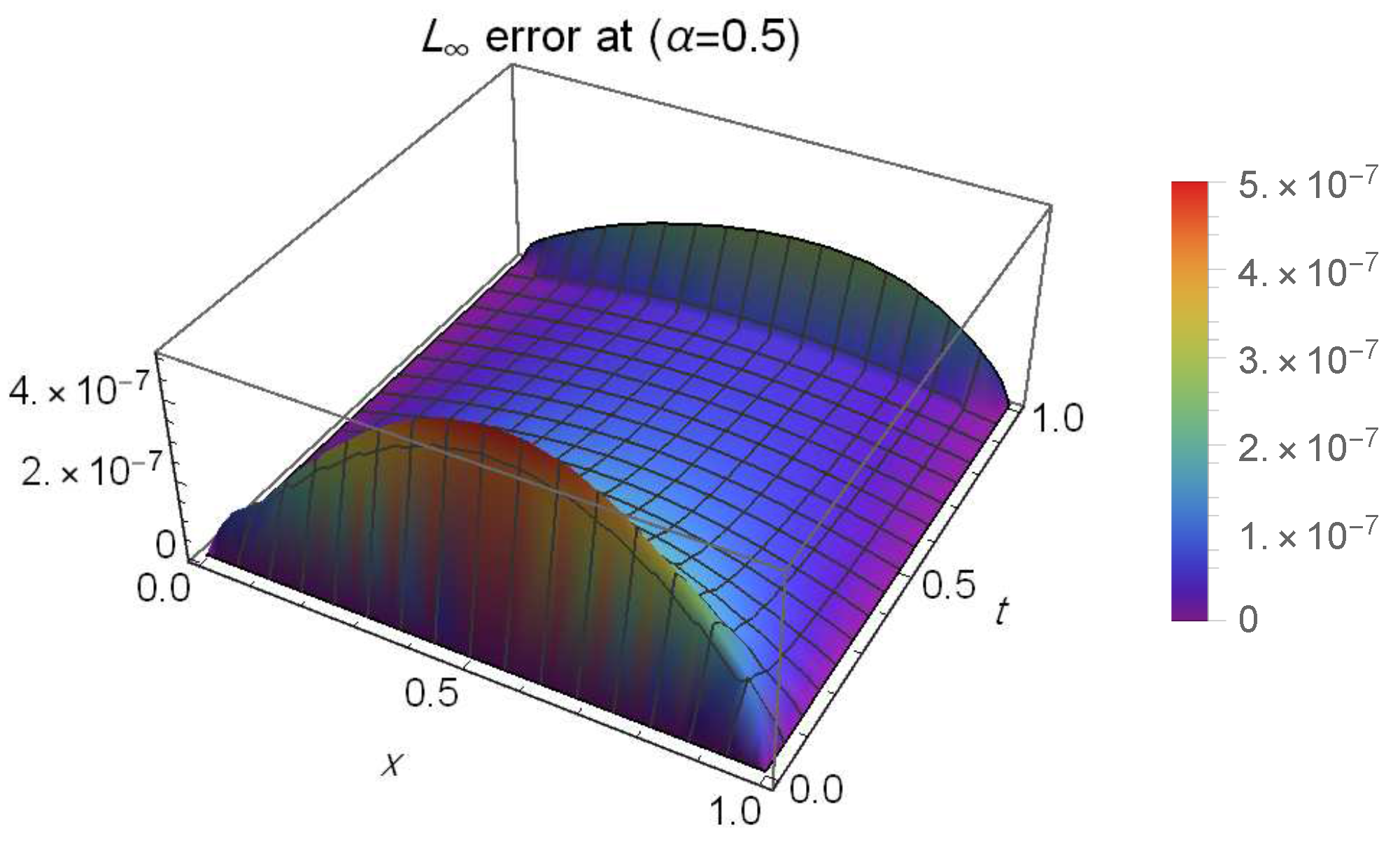
In Table 5, the absolute errors for the case corresponding to $N=18,$ $\alpha =0.1$, and $\alpha =0.9$ are displayed. This table confirms that the presented method has high performance and produces accurate results. In addition, Figure 3 illustrates the $L_{\infty }$ error for $\alpha =0.5$ at $N=18$. The results show good agreement between the approximate solution and the exact one.

Table 5. The absolute errors for Example 3.

	$\mathit{\alpha }=0.1$			$\mathit{\alpha }=0.9$
$\mathbf{x}$	$\mathit{t}=\frac{\mathbf{1}}{\mathbf{10}}$	$\mathit{t}=\frac{\mathbf{5}}{\mathbf{10}}$	$\mathit{t}=\frac{\mathbf{9}}{\mathbf{10}}$	$\mathit{t}=\frac{\mathbf{1}}{\mathbf{10}}$	$\mathit{t}=\frac{\mathbf{5}}{\mathbf{10}}$	$\mathit{t}=\frac{\mathbf{9}}{\mathbf{10}}$
0.1	$7.51088\times {10}^{-9}$	$3.37811\times {10}^{-10}$	$1.94761\times {10}^{-10}$	$6.06613\times {10}^{-7}$	$3.43728\times {10}^{-7}$	$2.23961\times {10}^{-7}$
0.2	$1.42794\times {10}^{-8}$	$6.40815\times {10}^{-10}$	$3.11168\times {10}^{-10}$	$1.11602\times {10}^{-6}$	$6.33681\times {10}^{-7}$	$4.13436\times {10}^{-7}$
0.3	$1.96572\times {10}^{-8}$	$8.81388\times {10}^{-10}$	$3.47166\times {10}^{-10}$	$1.51426\times {10}^{-6}$	$8.60691\times {10}^{-7}$	$5.63444\times {10}^{-7}$
0.4	$2.31269\times {10}^{-8}$	$1.03444\times {10}^{-9}$	$1.34724\times {10}^{-8}$	$1.78783\times {10}^{-6}$	$1.01624\times {10}^{-6}$	$6.84415\times {10}^{-7}$
0.5	$2.43513\times {10}^{-8}$	$1.04202\times {10}^{-9}$	$1.32679\times {10}^{-7}$	$1.92288\times {10}^{-6}$	$1.09187\times {10}^{-6}$	$1.04649\times {10}^{-6}$
0.6	$2.32053\times {10}^{-8}$	$5.93031\times {10}^{-10}$	$9.68495\times {10}^{-7}$	$1.90517\times {10}^{-6}$	$1.07976\times {10}^{-6}$	$3.98943\times {10}^{-6}$
0.7	$1.97889\times {10}^{-8}$	$2.20531\times {10}^{-9}$	$5.43109\times {10}^{-6}$	$1.72122\times {10}^{-6}$	$9.76103\times {10}^{-7}$	$2.04777\times {10}^{-5}$
0.8	$1.44202\times {10}^{-8}$	$1.35044\times {10}^{-8}$	$1.94111\times {10}^{-5}$	$1.35221\times {10}^{-6}$	$7.49924\times {10}^{-7}$	$5.23308\times {10}^{-5}$
0.9	$7.60732\times {10}^{-9}$	$4.18981\times {10}^{-8}$	$5.25662\times {10}^{-5}$	$7.86145\times {10}^{-7}$	$8.31597\times {10}^{-7}$	$6.27135\times {10}^{-5}$

Figure 3. Th $L_{\infty }$ error for Example 3.

6. Concluding Remarks

The nonlinear FRSE was treated numerically by applying the spectral Galerkin method using some polynomials related to shifted sixth-kind Chebyshev polynomials as basis functions. The proposed problem is reduced to a nonlinear system of algebraic equations that can be solved using Newton’s iterative method. The resulting approximate solutions using the suggested method are extremely close to the exact ones, indicating that our proposed algorithm can efficiently solve the problem. To demonstrate the validity and enormous potential of the algorithm, comparisons are performed between our proposed approximate solutions and those developed by other methods in the literature. In this paper, Wolfram Mathematica 11.2 was used for all calculations. In future work, we think that the theoretical results in this paper will be useful for other types of differential equations. In addition, we think that we can derive other derivative formulas for some polynomials related to Chebyshev polynomials of the sixth kind, in order to handle types of fractional differential equations that involve terms of other high-order derivatives.

References

- Fetecu, C.; Fetecu, C. The Rayleigh–Stokes problem for heated second grade fluids. Int. J. Non-Linear Mech. 2002, 37, 1011–1015. [Google Scholar] [CrossRef]
- Shen, F.; Tan, W.; Zhao, Y.; Masuoka, T. The Rayleigh–Stokes problem for a heated generalized second grade fluid with fractional derivative model. Nonlinear Anal. Real World Appl. 2006, 7, 1072–1080. [Google Scholar] [CrossRef]
- Abelman, S.; Hayat, T.; Momoniat, E. On the Rayleigh problem for a Sisko fluid in a rotating frame. Appl. Math. Comput. 2009, 215, 2515–2520. [Google Scholar] [CrossRef]
- Gabriele, A.; Spyropoulos, F.; Norton, I.T. Kinetic study of fluid gel formation and viscoelastic response with kappa-carrageenan. Food Hydrocoll. 2009, 23, 2054–2061. [Google Scholar] [CrossRef]
- Guan, Z.; Wang, X.; Ouyang, J. An improved finite difference/finite element method for the fractional Rayleigh–Stokes problem with a nonlinear source term. J. Appl. Math. Comput. 2021, 65, 451–479. [Google Scholar] [CrossRef]
- Dehghan, M.; Abbaszadeh, M. A finite element method for the numerical solution of Rayleigh–Stokes problem for a heated generalized second grade fluid with fractional derivatives. Eng. Comput. 2017, 33, 587–605. [Google Scholar] [CrossRef]
- Nikan, O.; Golbabai, A.; Machado, J.A.T.; Nikazad, T. Numerical solution of the fractional Rayleigh–Stokes model arising in a heated generalized second-grade fluid. Eng. Comput. 2021, 37, 1751–1764. [Google Scholar] [CrossRef]
- Hafez, R.M.; Zaky, M.A.; Abdelkawy, M.A. Jacobi spectral Galerkin method for distributed-order fractional Rayleigh–Stokes problem for a generalized second grade fluid. Front. Phys. 2020, 7, 240. [Google Scholar] [CrossRef]
- Zaky, M.A. An improved tau method for the multi-dimensional fractional Rayleigh–Stokes problem for a heated generalized second grade fluid. Comput. Math. Appl. 2018, 75, 2243–2258. [Google Scholar] [CrossRef]
- Xue, C.; Nie, J. Exact solutions of the Rayleigh–Stokes problem for a heated generalized second grade fluid in a porous half-space. Appl. Math. Model. 2009, 33, 524–531. [Google Scholar] [CrossRef]
- Chen, C.; Liu, F.; Anh, V. Numerical analysis of the Rayleigh–Stokes problem for a heated generalized second grade fluid with fractional derivatives. Appl. Math. Comput. 2008, 204, 340–351. [Google Scholar] [CrossRef] [Green Version]
- Abd-Elhameed, W.M.; Doha, E.H.; Youssri, Y.H.; Bassuony, M.A. New Tchebyshev-Galerkin operational matrix method for solving linear and nonlinear hyperbolic telegraph type equations. Numer. Methods Partial Differ. Equ. 2016, 32, 1553–1571. [Google Scholar] [CrossRef]
- Zhou, F.; Xu, X. The third kind Chebyshev wavelets collocation method for solving the time-fractional convection diffusion equations with variable coefficients. Appl. Math. Comput. 2016, 280, 11–29. [Google Scholar] [CrossRef]
- Doha, E.H.; Abd-Elhameed, W.M.; Bassuony, M.A. On the coefficients of differentiated expansions and derivatives of Chebyshev polynomials of the third and fourth kinds. Acta Math. Sci. 2015, 35, 326–338. [Google Scholar] [CrossRef]
- Masjed-Jamei, M. Some New Classes of Orthogonal Polynomials and Special Functions: A Symmetric Generalization of Sturm-Liouville Problems and Its Consequences. Ph.D. Thesis, University of Kassel, Department of Mathematics, Kassel, Germany, 2006. [Google Scholar]
- Xu, Y. An integral formula for generalized Gegenbauer polynomials and Jacobi polynomials. Adv. Appl. Math. 2002, 29, 328–343. [Google Scholar] [CrossRef] [Green Version]
- Draux, A.; Sadik, M.; Moalla, B. Markov—Bernstein inequalities for generalized Gegenbauer weight. Appl. Numer. Math. 2011, 61, 1301–1321. [Google Scholar] [CrossRef]
- Xu, X.; Xiong, L.; Zhou, F. Solving fractional optimal control problems with inequality constraints by a new kind of Chebyshev wavelets method. J. Comput. Sci. 2021, 54, 101412. [Google Scholar] [CrossRef]
- Babaei, A.; Jafari, H.; Banihashemi, S. Numerical solution of variable order fractional nonlinear quadratic integro-differential equations based on the sixth-kind Chebyshev collocation method. J. Comput. Appl. Math. 2020, 377, 112908. [Google Scholar] [CrossRef]
- Jafari, H.; Babaei, A.; Banihashemi, S. A novel approach for solving an inverse reaction–diffusion–convection problem. J. Optim. Theory Appl. 2019, 183, 688–704. [Google Scholar] [CrossRef]
- Abd-Elhameed, W.M.; Youssri, Y.H. Sixth-kind Chebyshev spectral approach for solving fractional differential equations. Int. J. Nonlinear Sci. Numer. Simul. 2019, 20, 191–203. [Google Scholar] [CrossRef]
- Abd-Elhameed, W.M. Novel expressions for the derivatives of sixth kind Chebyshev polynomials: Spectral solution of the non-linear one-dimensional Burgers’ equation. Fractal Fract. 2021, 5, 53. [Google Scholar] [CrossRef]
- Sadri, K.; Aminikhah, H. A new efficient algorithm based on fifth-kind Chebyshev polynomials for solving multi-term variable-order time-fractional diffusion-wave equation. Int. J. Comput. Math. 2022, 99, 966–992. [Google Scholar] [CrossRef]
- Abd-Elhameed, W.M.; Youssri, Y.H. Fifth-kind orthonormal Chebyshev polynomial solutions for fractional differential equations. Comput. Appl. Math. 2018, 37, 2897–2921. [Google Scholar] [CrossRef]
- Atta, A.G.; Moatimid, G.M.; Youssri, Y.H. Generalized Fibonacci operational tau algorithm for fractional Bagley-Torvik equation. Prog. Fract. Differ. Appl. 2020, 6, 215–224. [Google Scholar]
- Faghih, A.; Mokhtary, P. An efficient formulation of Chebyshev tau method for constant coefficients systems of multi-order FDEs. J. Sci. Comput. 2020, 82, 6. [Google Scholar] [CrossRef]
- Atta, A.G.; Abd-Elhameed, W.M.; Moatimid, G.M.; Youssri, Y.H. Shifted fifth-kind Chebyshev Galerkin treatment for linear hyperbolic first-order partial differential equations. Appl. Numer. Math. 2021, 167, 237–256. [Google Scholar] [CrossRef]
- Podlubny, I. Fractional Differential Equations: An Introduction to Fractional Derivatives, Fractional Differential Equations, to Methods of Their Solution and Some of Their Applications; Academic Press: San Diego, CA, USA, 1999. [Google Scholar]
- Atta, A.G.; Abd-Elhameed, W.M.; Moatimid, G.M.; Youssri, Y.H. Advanced shifted sixth-kind Chebyshev tau approach for solving linear one-dimensional hyperbolic telegraph type problem. Math. Sci. 2022. [Google Scholar] [CrossRef]
- Stewart, J. Single Variable Essential Calculus: Early Transcendentals; Cengage Learning: Boston, MA, USA, 2012. [Google Scholar]
Publisher’s Note: MDPI stays neutral with regard to jurisdictional claims in published maps and institutional affiliations. |
© 2022 by the authors. Licensee MDPI, Basel, Switzerland. This article is an open access article distributed under the terms and conditions of the Creative Commons Attribution (CC BY) license (https://creativecommons.org/licenses/by/4.0/).