Conservative Finite-Difference Scheme for 1D Ginzburg–Landau Equation

Abstract

In this study, our attention is focused on deriving integrals of motion (conservation laws; invariants) for the problem of an optical pulse propagation in an optical fiber containing an optical amplifier or attenuator because, to date, such invariants are absent in the literature. The knowledge of a problem’s invariants allows us develop finite-difference schemes possessing the conservativeness property, which is crucial for solving nonlinear problems. Laser pulse propagation is governed by the nonlinear Ginzburg–Landau equation. Firstly, the problem’s conservation laws are developed for the various parameters’ relations: for a linear case, for a nonlinear case without considering the linear absorption, and for a nonlinear case accounting for the linear absorption and homogeneous shift of the pulse’s phase. Hereafter, the Crank–Nicolson-type scheme is constructed for the problem difference approximation. To demonstrate the conservativeness of the constructed implicit finite-difference scheme in the sense of preserving difference analogs of the problem’s invariants, the corresponding theorems are formulated and proved. The problem of the finite-difference scheme’s nonlinearity is solved by means of an iterative process. Finally, several numerical examples are presented to support the theoretical results.

1. Introduction

It is well known that the Ginzburg–Landau equation (GLE) was introduced in the scientific literature in the middle of the 20th century as a developing theory of superconductivity [1,2]. To date, the GLE has been widely used in the physics fields of superconductivity and superfluidity [3,4,5,6,7,8,9,10,11]. The GLE is used also for describing a number of nonlinear phenomena [12,13,14,15,16,17,18,19,20,21,22,23,24,25,26,27,28,29,30,31], such as biophysics systems, nonlinear phenomena in liquid crystals, spatio-temporal chaos, oscillations of different nature (see review papers [32,33,34], where associated references can be found). Additionally, the GLE plays an essential role in nonlinear optics. To our knowledge, its first application in this field of laser physics was presented in [35], and then this equation was used for describing nonlinear optical phenomena (see, for example, [36,37,38,39,40,41]). It should be stressed that, in this case, the equation is written with respect to the so-called slowly varying complex amplitude and does not contain the vector potential of the electro-magnetic field before the terms referring to the second-order derivative on spatial coordinates.

Due to a complexity of the partial differential equations, such as GLE, and nonlinear Schrödinger equation (NLSE), Gross–Pitaevskii equation, Klein–Gordon equation, and Korteweg–De Vries equation, and others, the exact solutions can be obtained only in particular cases or maybe with strict assumptions. Therefore, solving these problems via computer simulations is an attractive issue and many numerical methods have been proposed and investigated [42,43,44,45,46,47,48,49,50,51,52,53,54,55,56,57,58,59,60,61].

One of the crucial features of the finite-difference scheme (FDS) used for solving nonlinear time-dependent problems is the conservativeness property. This means that a numerical method possesses the difference analogs of the problem’s conservation laws (invariants). It is known that conservativeness is a necessary condition of the FDS’s convergence (the convergence of a numerical solution to those of differential problems) for solving problems with discontinuous coefficients [48]. The conservativeness of the numerical method is of great importance because its validity guarantees the accordance of a numerical solution with its physical sense, especially this is required for nonlinear problems. The main advantage of conservative FDSs consists of possessing asymptotic numerical stability. On the contrary, the use of nonconservative schemes may lead to the numerical solution of NLSE divergence [49]. The significance that accounts for the conservation laws, such as energy invariants or the Hamiltonian, for numerical algorithm construction is discussed in [50]. In that study, it is emphasized that, for some problems, the conservativeness property of the scheme is “a criterion to judge the success of a numerical simulation” and it has a primary importance.

Therefore, many authors have directed their efforts towards developing conservative FDSs for a solution of the nonlinear problem. Among them we emphasize the problem of finding numerical solutions of the NLSE [49,50,51,52,53,54,55,56,57,58,59,60,61]. In [51], a splitting method for the cubic NLSE on a torus that possesses a long-time near-conservation of energy is applied and investigated. In [52], to solve coupled NLSEs, a linearly implicit conservative method that precisely conserves the energy is presented. It is stated that the energy’s preservation rules out any possibility of the numerical solution distortion. In [53], the two discrete conservative laws were obtained for the NLSE involving a quintic term, and a compact FDS was presented. Two compact FDSs for a one-dimensional cubic nonlinear Schrödinger equation were proposed in [54]. Both schemes were proven to conserve discrete mass and energy.

It should be emphasized that most articles devoted to FDSs only conserve the energy’s invariant. However, to enhance the accuracy of the numerical solution, the development of fully conservative FDSs that conserve all problem invariants is required. Therefore, information about the wave front of a beam and frequency modulation of a pulse, as well as the terms referring to the second-order dispersion and beam diffraction, is contained in Hamiltonian (the so-called third invariant), but this information is absent in the energy invariant. In [55], a conservative FDS for the numerical solution of the Gross–Pitaevskii equation was proposed. It preserves three invariants of the problem: the $L_2$-norm of the solution, the impulse functional, and the energy functional. The comparison of several numerical examples demonstrated its advantages over some well-known and widely used methods. A linearized and decoupled compact FDS for the coupled Gross–Pitaevskii system was studied in [56]. It was proven that this new scheme preserves the three invariants in the discrete sense: not only the total mass and energy, but also the magnetization. In [57], it was shown that the use of energy-conserving methods (Hamiltonian Boundary Value Methods) were able to conserve a discrete counterpart of the Hamiltonian functional at solving NLSEs. Such an approach conferred more robustness on the numerical solution of such a problem. The objective of study [58] is to investigate the possibility of developing numerical schemes for the general NLSE that simultaneously conserve mass and energy. In that study it is stated in the present study that “The quality of the numerical approximation hence hinges on how well the conserved integrals can be preserved at the discrete level. Numerical methods without this property may result in substantial phase and shape errors after long time integration.” A family of mass- and energy-conserved time-stepping schemes are constructed, and it is shown that the proposed schemes preserve both mass and energy without any mesh restriction. In [59], the different splitting algorithms for numerical solutions of both classical and generalized NLSEs are presented and analyzed. The problem’s discrete conservation laws are used to test the accuracy of the discrete solution in numerical experiments. In [60], the conservation laws for generalized NLSEs in the framework of slowly evolving wave approximation are derived based on an original transformof the NLSEs. The energy’s invariant, the spectral invariant, the Hamiltonian, and some other invariants are also presented. It is demonstrated that, to avoid the development of the nonphysical solution’s instability, it is necessary to consider the spectral invariant for providing computer simulations. In [61,62], the comparison of the efficiency of several conservative and splitting FDSs is provided. In [61], conservative FDSs are constructed for the problem of femtosecond pulse propagation in an optical fiber, considering the time derivative of the medium nonlinear response. The proposed FDSs preserve several invariants involving both the intensity profile of the beam and the phase distribution of the beam. In [62], for the set of 1D-coupled NLSEs, two conservative FDSs are constructed. Each of them preserves one of two differential problem’s invariants (the energy’s invariant or the Hamiltonian), while another is preserved with the second order of approximation. It was shown that the accuracy of the computer simulation results depends on which of the problem’s invariants is preserved: the Hamiltonian is more preferable because it contains both a phases and intensities of interacting waves.

Turning to the GLE numerical solution, it should be stressed that, to the best of our knowledge, the conservation laws (integrals of motion) of this equation are absent in the literature (even for the linear case), despite extensive studies on the numerical methods having been conducted [63,64,65,66,67,68,69,70,71,72,73,74,75,76,77]. For developing difference schemes for the GLE solution, splitting methods (Strang splitting and alternating direction methods) were mostly used and the authors usually focused on the investigation of their convergence conditions and accuracy order.

In [63], the three-layer FDS, which approximates the GLE with the second order on a time coordinate and fourth order on a spatial coordinate, was developed. The work is devoted to the investigation of FDS stability and approximation accuracy. In [64], the constructing artificial boundary conditions at three-dimensional simulations of the vortex phenomena in superconductors is discussed. In [65], the authors compared the performance of several numerical algorithms for the GLE solution. In [66], the finite-difference method was implemented to solve the complex 2D GLE. The conditions of the FDS convergence and its approximation order were studied. The method seems to be an efficient tool for solving problems in domains of complicated geometry. Papers [67,68,69,70,71,72] were devoted to studying the stability of the GLE solution and its invariant solution for the chosen gauge and developing FDS for a numerical solution of the GLE involving the nonlocal nonlinear response of a medium. Paper [73] deals with the time-depended Landau–Khalatnikov equation modified in view of the Landau–Ginzburg–Devonshire approach. For its solving, a computational scheme based on a monotone and absolutely stable implicit finite-difference method of the second-order accuracy is proposed. The fractional GLEs are considered in [74,75,76,77]. In [74], an alternating direction implicit scheme was applied to the two-dimensional spatial fractional GLE. Its convergence properties were derived under some conditions. In [75], a novel fourth-order fractional compact difference operator in space and the Crank–Nicolson method in time were proposed for the nonlinear space fractional GLE solution. Some new techniques and important lemmas were developed to prove the unique solvability, stability, and convergence in the sense of different norms.

In [76], a three-level linearized FDS for the high-dimensional nonlinear GLE with fractional Laplacian was proposed. The unique solvability and boundedness of the solution of the FDS were analyzed, and its unconditionally stability and second-order accuracy in time and space were demonstrated. A numerical integration method for the space fractional GLE is proposed in [77]. The differential equation was split into two subproblems (linear and nonlinear ones), which were solved by the dynamical low-rank approach, and the convergence of the method was rigorously proven. However, none of these studies investigated numerical approaches from the standpoint of their conservativeness; meanwhile, this property was of crucial importance. In this regard, the development of conservation laws for the GLE is a challenging task and it is the objective of this study. The problem’s invariants allow us to construct conservative FDSs and verify this property implementation at the numerical simulations: accuracy of the invariant’s preservation can be used to assess both the accuracy and adequacy of the obtained numerical solution.

The remainder of this study is organized as follows. Section 2 consists of the statement of the differential problem and description of all involved parameters. In Section 3, we derive the problem’s invariants separately for the linear case and two nonlinear cases, and formulate the corresponding theorems. Section 4 is devoted to constructing the FDS, which is based on the Crank–Nicolson scheme. Because the FDS is nonlinear, an iterative process for its realization is applied. In Section 5, we formulate and proove the theorems devoted to the conservativeness of the constructed FDS in the sense of preserving the difference analog of the problem’s invariant. To support the theoretical investigation, the computer simulation results are presented in Section 6. On the basis of numerical experiments, the conservativeness of the constructed FDS is also demonstrated. Finally, the paper is summarized with a short conclusions.

2. Problem Statement

Let us consider an optical pulse propagation in a spatio-temporal domain $G_0=(0,L_z]\times (0,L_t)$ of a nonlinear medium. For the process description, the following features are taken into account: a bounded frequency bandwidth of the transmission spectrum of a medium, the difference between the pulse’s carrier frequency and a central frequency of the transmission spectrum of a medium, a linear absorption (or amplification) of the optical pulse energy, a homogeneous phase shift of the wave packet at its propagation along the z-coordinate, the two-photon absorption (or nonlinear amplification), and the Kerr effect. The problem under consideration is described by the following dimensionless nonlinear GLE [35,36], with respect to the slowly varying envelope of the wave packet:

$$\begin{array}{c}\frac{\partial A}{\partial z}+(\nu +i·{\nu }_{\omega })·\frac{\partial A}{\partial t}+(i·D_2+D_{2\omega })·\frac{{\partial }^{2}A}{\partial t^2}+(\delta +i·\alpha ){\left|A\right|}^{2}A+(0.5·{\delta }_0+i·n_0)A=0\end{array}, (z,t)\in G_0.$$

(1)

The initial and uniform Dirichlet boundary conditions (BCs) are stated as follows:

$$\begin{array}{c}A(z=0,t)=\end{array}{A}_0(t), t\in \left[0,L_t\right],$$

(2)

$$\begin{array}{c}A(z,0)= A(z,L_t)=0\end{array}, z\in \left[0,L_z\right].$$

(3)

They correspond to a finite initial distribution of the optical pulse on a time coordinate that is the ordinary proposition for the problems of nonlinear optics.

The spatial z-coordinate denotes a longitudinal coordinate along which the pulse propagates, and it is measured in the pulse’s dispersion length. Parameter $L_z$ denotes the optical pulse-propagation distance. In turn, time $t$ is measured in units of the incident pulse duration. $L_t$ denotes a time interval that is chosen in such a way that the complex amplitude $A(z,t)$ of the pulse is equal to zero during some time interval near the boundary’s values $t=0,L_t$. It can always be performed because the initial distribution of the complex amplitude is finite, and the distance of the optical pulse’s propagation is bounded. Let us stress that this proposition will be used to prove the conservativeness of the developed FDS.

In (1)–(3), the function $A(z,t)$ denotes a slowly varying complex amplitude of the optical pulse that is normalized by the square root of the maximal incident pulse intensity $I_{in}^{0.5}$. Symbol $i$ denotes imaginary unity: $i^2=-1$. The parameter $\nu$ characterizes the pulse’s group velocity, and parameter ${\nu }_{\omega }$ characterizes a shift in the carrier frequency of the wave packet in the frequency domain. Coefficient $D_2$ characterizes the pulse’s group velocity dispersion (second-order dispersion). Negativity (positivity) of $D_2$ corresponds to the normal (anomalous) dispersion. Parameter $D_{2\omega }$ characterizes a range of the frequencies, which are absorbed (amplified) at the optical pulse propagation, and it is proportional to the squared inverse bandwidth of the transmission spectrum of a medium. Parameter $\delta$ describes the nonlinear gain (or absorption), and parameter $\alpha$ describes the pulse’s self-phase modulation. Let us note that, if $\alpha >0$, then the pulse compression occurs in a medium with an anomalous dispersion. Parameter ${\delta }_0$ describes the linear absorption (or amplification) of a medium, and parameter $n_0$ is responsible for the homogeneous phase shift of the pulse at its propagation.

3. Invariant of the Problem

Below, we consider separately various particular cases of the GLE (1).

3.1. Linear Problem: $\delta =\alpha =0$

Let us consider the problem (1)–(3) in a linear medium. In this case, there is:

Theorem 1.

The problem (1)–(3) in a linear case ($\delta =\alpha =0$) possesses the following invariant:

$$J_p(z)=\begin{array}{c}\underset{0}{\overset{L_t}{{\displaystyle \int }}}P(z,t)·A(z,t)dt=e^{-2·(0.5{\delta }_0+i·n_0)z}\underset{0}{\overset{L_t}{{\displaystyle \int }}}P(0,t)·A(0,t)dt\end{array},$$

(4a)

or

$$\begin{array}{c}{P}^2(z,L_t)=e^{-2·(0.5{\delta }_0+i·n_0)z}{P}^2(0,L_t)\end{array}$$

(4b)

or

$$\begin{array}{c}P(z,L_t)=e^{-(0.5{\delta }_0+i·n_0)z}P(0,L_t)\end{array},$$

(4c)

where the function $\begin{array}{c}P(z,t)\end{array}$ is defined as follows:

$$\begin{array}{c}P(z,t)=\underset{0}{\overset{t}{{\displaystyle \int }}}A(z,\xi )d\xi .\end{array}$$

(5)

Evidently, the following BCs and initial condition

$$\begin{array}{c}P(z,0)=0, \frac{\partial P(z,L_t)}{\partial t}=0, z\in [0,L_z]\end{array},$$

(6)

$$\begin{array}{c}P(0,t)=\underset{0}{\overset{t}{{\displaystyle \int }}}{A}_0(\xi )d\xi \end{array}$$

(7)

are valid for the introduced function.

Proof. 

Integrating each term of Equation (1) with zero value of the parameters $\delta =\alpha =0,$ easily to obtain the following equation:

$$\begin{array}{c}\frac{\partial P}{\partial z}+\left(\nu +i·{\nu }_{\omega }\right)·\frac{\partial P}{\partial t}+\left(i·D_2+D_{2\omega }\right)·\frac{{\partial }^{2}P}{\partial t^2}+(0.5{\delta }_0+i·n_0)P=0\end{array}.$$

(8)

In the next step, we multiply Equation (1) by $P$ and multiply Equation (8) by $A.$ Then, we summarize the results of the multiplication and take the integral from the sum on the time coordinate. As a result, we obtain the following equation:

$$\begin{array}{l}\frac{\partial }{\partial z}\underset{0}{\overset{L_t}{{\displaystyle \int }}}P(z,t)A(z,t)dt+\left(\nu +i·{\nu }_{\omega }\right)·\underset{0}{\overset{L_t}{{\displaystyle \int }}}\left(\frac{\partial A(z,t)}{\partial t}P(z,t)+\frac{\partial P(z,t)}{\partial t}A(z,t)\right)dt\\ +\left(D_{2\omega }+i·D_2\right)·\underset{0}{\overset{L_t}{{\displaystyle \int }}}\left(\frac{{\partial }^{2}A(z,t)}{\partial t^2}P(z,t)+\frac{{\partial }^{2}P(z,t)}{\partial t^2}A(z,t)\right)dt\\ +2·(0.5{\delta }_0+i·n_0)·\underset{0}{\overset{L_t}{{\displaystyle \int }}}P(z,t)·A(z,t)·dt=0.\end{array}$$

(9)

Equation (9) can be simplified using an integration by parts:

$$\begin{array}{l}\frac{\partial }{\partial z}\underset{0}{\overset{L_t}{{\displaystyle \int }}}P(z,t)·A(z,t)·dt+\left(D_{2\omega }+i·D_2\right)·{\left[\frac{\partial A(z,t)}{\partial t}P(z,t)+\frac{\partial P(z,t)}{\partial t}A(z,t)\right]|}_0^{L_t}\\ -\left(D_{2\omega }+i·D_2\right)·{\left[A^2(z,t)\right]|}_0^{L_t}+2·\left(\nu +i·{\nu }_{\omega }\right)·{\left[A(z,t)·P(z,t)\right]|}_0^{L_t}\\ +2·(0.5{\delta }_0+i·n_0)·\underset{0}{\overset{L_t}{{\displaystyle \int }}}P(z,t)·A(z,t)·dt=0.\end{array}$$

(10)

Accounting for the zero value of the complex amplitude near the time domain boundaries, the following equation occurs:

$$\begin{array}{c}\frac{\partial }{\partial z}\underset{0}{\overset{L_t}{{\displaystyle \int }}}P(z,t)·A(z,t)dt+\end{array}2·(0.5{\delta }_0+i·n_0)·\underset{0}{\overset{L_t}{{\displaystyle \int }}}P(z,t)·A(z,t)·dt=0.$$

(11)

Evidently, it means that the conservation law (4a), (4b) occurs.  □

Remark 1. 

Using substitution$\begin{array}{c}A(z,t)=\overline{A}(z,t)·e^{-(0.5{\delta }_0+i·n_0)z}\end{array}$, it is easy to transform Equation (1) with$\delta =\alpha =0$to the form without the last term. Therefore, for the function$\begin{array}{c}\overline{A}(z,t)\end{array}$(and, consequently, for the function$\begin{array}{c}\overline{P}(z,t)\end{array}$, introduced in accordance with rule (5)), the equalities similar to (4a), (4b) occur without the exponential term.

Remark 2. 

The invariant (4c) can be obtained from Equation (1)by integrating this equation on the time coordinate with integration limits $t=0,L_t$, followed by the integration on the z-coordinate.

3.2. Nonlinear Problem without the Terms Describing the Linear Absorption (Amplification) of the Optical Energy and Homogeneous Phase Shift of the Optical Pulse: ${\delta }_0=n_0=0$

Let us consider the problem (1)–(3) at the optical pulse propagation in a nonlinear medium $\left(\delta \ne 0,\alpha \ne 0\right)$ without accounting for the linear absorption and homogeneous shift of the pulse’s phase $\left({\delta }_0=n_0=0\right)$. In this case, there is:

Theorem 2.

The problem (1)–(3) in a nonlinear case $\left(\delta \ne 0,\alpha \ne 0\right)$without the linear absorption and homogeneous shift of the pulse’s phase $\left({\delta }_0=n_0=0\right)$possesses the following invariant:

$$\begin{array}{c}P(z,L_t)=P(0,L_t)-\left(\delta +i\alpha \right)·\underset{0}{\overset{z}{{\displaystyle \int }}}\left(\underset{0}{\overset{L_t}{{\displaystyle \int }}}{\left|A(\xi ,t)\right|}^{2}A(\xi ,t)dt\right)d\xi \end{array}.$$

(12)

Proof. 

Integrating each term of Equation (1) with the zero value of the parameters $\left({\delta }_0=n_0=0\right)$, we obtain the following equation:

$$\begin{array}{c}\frac{\partial P}{\partial z}+\left(\nu +i·{\nu }_{\omega }\right)·\frac{\partial P}{\partial t}+\left(i·D_2+D_{2\omega }\right)·\frac{{\partial }^{2}P}{\partial t^2}+\left(\delta +i\alpha \right)\underset{0}{\overset{t}{{\displaystyle \int }}}{\left|A\left(z,\xi \right)\right|}^{2}A\left(z,\xi \right)d\xi =0\end{array}.$$

(13)

Subsequently, we multiply Equation (1) by $P$ and multiply Equation (13) by $A$. Then, we summarize the results of the multiplication and obtain the integral on the time coordinate. As a result, the following equation is obtained:

$$\begin{array}{c}\frac{\partial }{\partial z}\underset{0}{\overset{L_t}{{\displaystyle \int }}}P(z,t)·A(z,t)·dt+\left(\nu +i·{\nu }_{\omega }\right)·\underset{0}{\overset{L_t}{{\displaystyle \int }}}\left(\frac{\partial A(z,t)}{\partial t}P(z,t)+\frac{\partial P(z,t)}{\partial t}A(z,t)\right)dt\\ +\left(D_{2\omega }+i·D_2\right)·\underset{0}{\overset{L_t}{{\displaystyle \int }}}\left(\frac{{\partial }^{2}A(z,t)}{\partial t^2}P\left(z,t\right)+\frac{{\partial }^{2}P(z,t)}{\partial t^2}A(z,t)\right)dt\\ +\left(\delta +i\alpha \right)·\left\{\underset{0}{\overset{L_t}{{\displaystyle \int }}}\left({\left|A(z,t)\right|}^{2}A(z,t)·P(z,t)+\underset{0}{\overset{t}{{\displaystyle \int }}}{\left|A(z,\xi )\right|}^{2}A(z,\xi )d\xi ·A(z,t)\right)dt\right\}=0.\end{array}$$

(14)

The second and third terms of Equation (14) can be simplified in the same way as those of Equation (9). The last term can be transformed as follows:

$$\begin{array}{c}\frac{\partial }{\partial z}\underset{0}{\overset{L_t}{{\displaystyle \int }}}P(z,t)·A(z,t)·dt+\end{array}\left(\delta +i\alpha \right)·P(z,L_t)·\underset{0}{\overset{L_t}{{\displaystyle \int }}}{\left|A(z,t)\right|}^2·A(z,t)·dt=0$$

(15a)

or

$$P(z,L_t)·\left(\frac{\partial P(z,L_t)}{\partial z}+\left(\delta +i\alpha \right)·\underset{0}{\overset{L_t}{{\displaystyle \int }}}{\left|A(z,t)\right|}^2·A(z,t)·dt\right)=0.$$

(15b)

Evidently, one can obtain Equation (12) from Equation (15b) because, in general cases, the function $P\left(z,L_t\right)$ does not equal zero.  □

Remark 3. 

Invariant (12) can be obtained from Equation (1) by integrating this equation on the time coordinate with integration limits $t=0,L_t$and with the following integration on the z-coordinate.

3.3. Nonlinear Problem with the Linear Absorption (Amplification) of the Optical Energy and Homogeneous Shift of the Optical Pulse’s Phase: $\delta \ne 0,\alpha \ne 0,{\delta }_0\ne 0,n_0\ne 0$

Let us consider the problem (1)–(3) with the non-zero value of the equation’s coefficients characterizing the nonlinear and linear properties of a medium:$\left(\delta \ne 0,\alpha \ne 0,{\delta }_0\ne 0,n_0\ne 0\right)$. In this case, there is:

Theorem 3.

The problem (1) in a nonlinear case $\left(\delta \ne 0,\alpha \ne 0\right)$with the linear absorption and inhomogeneous shift of the pulse’s phase $\left({\delta }_0\ne 0,n_0\ne 0\right)$possesses the following invariant:

$$\frac{\partial P(z,L_t)}{\partial z}+(0.5{\delta }_0+i·n_0)·P(z,L_t)+\left(\delta +i\alpha \right)·\underset{0}{\overset{L_t}{{\displaystyle \int }}}{\left|A(z,t)\right|}^2·A(z,t)dt=0$$

(16a)

or

$$P(z,L_t)=\begin{array}{c}{e}^{-(0.5{\delta }_0+i·n_0)z}\left(P(0,L_t)-\left(\delta +i\alpha \right)·\underset{0}{\overset{z}{{\displaystyle \int }}}\begin{array}{c}{e}^{(0.5{\delta }_0+i·n_0)\xi }\end{array}\left(\underset{0}{\overset{L_t}{{\displaystyle \int }}}{\left|A(\xi ,t)\right|}^2·A(\xi ,t)·dt\right)d\xi \right)\end{array}.$$

(16b)

Proof. 

In the case under consideration, the evolution of function $P(z,t)$ is governed by the following equation:

$$\begin{array}{l}\frac{\partial P(z,t)}{\partial z}+\left(\nu +i·{\nu }_{\omega }\right)·\frac{\partial P(z,t)}{\partial t}+\left(i·D_2+D_{2\omega }\right)·\frac{{\partial }^{2}P(z,t)}{\partial t^2}\\ +(0.5{\delta }_0+i·n_0)·P(z,t)+\left(\delta +i\alpha \right)\underset{0}{\overset{t}{{\displaystyle \int }}}{\left|A(z,\xi )\right|}^2·A(z,\xi )·d\xi =0.\end{array}$$

(17)

As above, we multiply Equation (1) by $P$ and multiply Equation (17) by $A$. Then, we summarize the results of the multiplication and obtain the integral from the sum on the time coordinate. As a result, the following equation can be obtained:

$$\begin{array}{c}\frac{\partial }{\partial z}\underset{0}{\overset{L_t}{{\displaystyle \int }}}P\left(z,t\right)A\left(z,t\right)dt+\left(\nu +i·{\nu }_{\omega }\right)·\underset{0}{\overset{L_t}{{\displaystyle \int }}}\left(\frac{\partial A\left(z,t\right)}{\partial t}P\left(z,t\right)+\frac{\partial P\left(z,t\right)}{\partial t}A\left(z,t\right)\right)dt\\ +\left(D_{2\omega }+i·D_2\right)·\underset{0}{\overset{L_t}{{\displaystyle \int }}}\left(\frac{{\partial }^{2}A\left(z,t\right)}{\partial t^2}P\left(z,t\right)+\frac{{\partial }^{2}P\left(z,t\right)}{\partial t^2}A\left(z,t\right)\right)dt+2·(0.5{\delta }_0+i·n_0)·\underset{0}{\overset{L_t}{{\displaystyle \int }}}P\left(z,t\right)·A\left(z,t\right)·dt\\ +\left(\delta +i\alpha \right)·\left\{\underset{0}{\overset{L_t}{{\displaystyle \int }}}\left({\left|A\left(z,t\right)\right|}^{2}A\left(z,t\right)·P\left(z,t\right)+\underset{0}{\overset{t}{{\displaystyle \int }}}{\left|A\left(z,\xi \right)\right|}^{2}A\left(z,\xi \right)d\xi ·A\left(z,t\right)\right)dt\right\}=0.\end{array}$$

(18)

Using algebra similar to that presented above, we transform Equation (18) into the following form:

$$\begin{gathered} \frac{\partial }{\partial z}\underset{0}{\overset{L_t}{{\displaystyle \int }}}P\left(z,t\right)A\left(z,t\right)dt+2·(0.5{\delta }_0+i·n_0)·\underset{0}{\overset{L_t}{{\displaystyle \int }}}P\left(z,t\right)·A\left(z,t\right)·dt+ \\ \left(\delta +i\alpha \right)·P\left(z,L_t\right)·\underset{0}{\overset{L_t}{{\displaystyle \int }}}{\left|A\left(z,t\right)\right|}^{2}A\left(z,t\right)dt=0. \end{gathered}$$

(19)

Therefore, we obtain the following equation:

$$P\left(z,t\right)\left(\frac{\partial P\left(z,L_t\right)}{\partial z}+(\frac{{\delta }_0}{2}+i·n_0)·P\left(z,L_t\right)\begin{array}{c}+\end{array}\left(\delta +i\alpha \right)·\underset{0}{\overset{L_t}{{\displaystyle \int }}}{\left|A\left(z,t\right)\right|}^{2}A\left(z,t\right)dt\right)=0.$$

(20)

Evidently, Equations (16a) and (16b) follow from Equation (20).  □

Remark 4. 

The invariant (14a) can be obtained from Equation (1) by integrating this equation on the time coordinate with integration limits $t=0,L_t$and with the following integration on the z-coordinate.

It should be stressed that, if an optical energy absorption is absent, then the energy of the optical pulse

$$\begin{array}{c}E\left(z\right)=\underset{0}{\overset{L_t}{{\displaystyle \int }}}{\left|A\left(z,t\right)\right|}^{2}dt\end{array}$$

does not change at its propagation. It means that the energy’s invariant occurs.

4. Finite-Difference Scheme and Iterative Method for Its Realization

In the domain $G=[0,L_z]\times [0,L_t]$ we introduce the uniform mesh $\mathsf{\Omega }={\omega }_z\times {\omega }_t$:

$${\omega }_z=\left\{z_m=mh, m=0,\dots ,N_z, h=\frac{L_z}{N_z}\right\}, {\omega }_t=\left\{t_l=l\tau , l=0,\dots ,N_t, \tau =\frac{L_t}{N_t}\right\},$$

where $h, \tau$ are mesh steps on spatial and time coordinates, respectively; $N_z, N_t$ are the number of mesh nodes in each of the coordinates. For writing the FDS, we use the following index-free notations for the mesh functions and operators:

$$\begin{array}{c}A=A_l=A(z_m,t_l) ,\widehat{A}={\widehat{A}}_l=A(z_m+h,t_l), \stackrel{0.5}{A}=0.5(A+\widehat{A}),\stackrel{0.5}{|A}{|}^2=0.5({\left|A\right|}^2+|\widehat{A}{|}^2),\\ A_{\stackrel{0}{t}}=\frac{A(z_m,t_{l+1})-A(z_m,t_{l-1})}{2\tau }, {\mathsf{\Lambda }}_{\overline{t}t}A=\frac{A(z_m,t_{l+1})-2A(z_m,t_l)+A(z_m,t_{l-1})}{{\tau }^2},\\ A_t=\frac{A(z_m,t_{l+1})-A(z_m,t_l)}{\tau },A_{\overline{t}}=\frac{A(z_m,t_l)-A(z_m,t_{l-1})}{\tau }.\end{array}$$

(21)

Let us note that, for brevity, here and below we use the same notation for the mesh function regarding the complex amplitude. Using (21), we approximate the problem (1)–(3) in the inner mesh nodes by the Crank–Nicolson-type FD:

$$\begin{array}{c}\frac{\widehat{A}-A}{h}+\left(\nu +i·{\nu }_{\omega }\right)·\stackrel{0.5}{A_{\stackrel{0}{t}}}+\left(i·D_2+D_{2\omega }\right)·{\mathsf{\Lambda }}_{\overline{t}t}\stackrel{0.5}{A}+\left(\delta +i·\alpha \right)·\stackrel{0.5}{|A}{|}^2\stackrel{0.5}{A}+(0.5{\delta }_0+i·n_0)\stackrel{0.5}{·A}=0.\end{array}$$

(22)

The initial condition (2) is approximated as follows:

$$\begin{array}{c}A\left(z_0,t_l\right)=A_0\left(t_l\right), l=\overline{0,N_t},\end{array}$$

(23)

and the BCs (3) are approximated as

$$\begin{array}{c}A\left(z_m,t_0\right)=0, A\left(z_m,t_{N_t}\right)=0, l=\overline{0,N_t}.\end{array}$$

(24)

It is easy to show that the developed FDSs possessed the second order of approximation on enough smooth solution of the differential problem.

Because the difference Equation (22) is nonlinear, the simple iteration method is applied, in which a nonlinear part of the equation is taken from the previous iteration:

$$\begin{array}{c}\frac{\stackrel{s+1}{\widehat{A}}-A}{h}+\left(\nu +i·{\nu }_{\omega }\right)\stackrel{s+1}{\stackrel{0.5}{A_{\stackrel{0}{t}}}}+\left(i·D_2+D_{2\omega }\right){\mathsf{\Lambda }}_{\overline{t}t}\stackrel{s+1}{\stackrel{0.5}{A}}+\left(\delta +i·\alpha \right)·|\stackrel{s}{\stackrel{0.5}{A}}{|}^2\stackrel{s}{\stackrel{0.5}{A}}+(0.5{\delta }_0+i·n_0)·\stackrel{s+1}{\stackrel{0.5}{A}}=0,\end{array}$$

(25)

where $s=0,1,2\dots$ is an iteration of numbers. The BCs for Equation (25) are written in a similar way as for Equation (22):

$$\begin{array}{c}\stackrel{s+1}{\widehat{A}}(z_m,t_0)=0,\stackrel{s+1}{\widehat{A}}(z_m,t_{N_t})=0, m=\overline{0,N_z}.\end{array}$$

(26)

The mesh function, belonging to the upper layer on the z-coordinate, is chosen at zero-value iteration (S = 0) equal to its value at the previous layer on the z-coordinate:

$$\stackrel{s=0}{\widehat{A}}=A.$$

(27)

The iteration process is terminated if the following inequality is valid:

$$\begin{array}{c}\stackrel{s+1}{|\widehat{A}}-\stackrel{s}{\widehat{A}|}\le {\epsilon }_1\stackrel{s}{\left|\widehat{A}\right|}+{\epsilon }_2, {\epsilon }_1,{\epsilon }_2=const>0, \forall t_l\in {\omega }_t\end{array}$$

(28)

To solve the tridiagonal systems of Equations (25) and (26), the Thomas algorithm was applied.

The difference analog of the energy’s integral is computed using the trapezoid rule, which possesses the second-order accuracy:

$$E(z_m)={\displaystyle \sum _{l=0}^{N_t}{\left|A\left(z_m,t_l\right)\right|}^2}\tau , m=\overline{0,N_z}.$$

(29)

5. Conservativeness of the Finite-Difference Scheme

The developed FDS was conservative. To prove this, we have to write the FDS for the mesh function $\begin{array}{c}P\left(z_m,t_l\right)\end{array}$ introduced on mesh $\mathsf{\Omega }$ and define the following notation:

$$\begin{array}{c}P=P_l=P\left(z_m,t_l\right)={\displaystyle {\displaystyle \sum }_{j=0}^l} \tau ·A\left(z_m,t_j\right), l=\overline{0,N_t}, m=\overline{0,N_z},\\ \widehat{P}={\widehat{P}}_l=P\left(z_m+h,t_l\right)={\displaystyle {\displaystyle \sum }_{j=0}^l} \tau ·A\left(z_m+h,t_j\right),l=\overline{0,N_t}, m=\overline{0,N_z-1},\\ \stackrel{0.5}{P}=0.5·(P+\widehat{P}),l=\overline{0,N_t}, m=\overline{0,N_z-1},\\ \frac{P\left(z_m,t_{l+1}\right)-P\left(z_m,t_l\right)}{\tau }=A\left(z_m,t_{l+1}\right),l=\overline{0,N_t-1}, m=\overline{0,N_z}.\end{array}$$

(30)

Firstly, we consider proving the theorem that is a difference analog of Theorem 1. We multiply Equation (22) by the mesh step $\tau$ and then summarize the values of mesh function $\tau A$ in mesh nodes $\overline{t_0,t_l}$. Using the notations introduced above, one can write the following FDS in the inner nodes of the mesh:

$$\begin{array}{c}\frac{\widehat{P}-P}{h}+\left(\nu +i·{\nu }_{\omega }\right)·\stackrel{0.5}{P_{\stackrel{0}{t}}}+\left(i·D_2+D_{2\omega }\right)·{\mathsf{\Lambda }}_{\overline{t}t}\stackrel{0.5}{P}+(0.5{\delta }_0+i·n_0)\stackrel{0.5}{·P}=0,\\ l=\overline{0,N_t-1}, m=\overline{0,N_z-1},\end{array}$$

(31)

the BCs (6) are approximated as follows:

$$\begin{array}{c}P\left(z_m,t_0\right)=0, P_{\overline{t}}\left(z_m,t_{N_t}\right)=0\end{array},m=\overline{0,N_z},$$

(32)

and the initial condition (7) is approximated in the following way:

$$\begin{array}{c}\begin{array}{c}P\left(z_0,t_l\right)={\displaystyle \sum _{j=0}^l} \tau ·A_0\left(t_j\right)\end{array}, l=\overline{0,N_t}\end{array}.$$

(33)

5.1. Linear Problem without Homogeneous Phase Shift and Absorption: $\delta =\alpha =0, {\delta }_0=n_0=0$

Firstly, we considered the optical pulse propagation in a linear medium without a homogeneous phase shift and absorption. The advisability of such a form of analysis concludes in proving the FDS’s conservativeness for the problem containing the last two linear terms in Equation (1). As we show below, despite the obvious, simple approximation of these terms, we met certain difficulties in proving the invariant of the FDS.

Theorem 4.

The FDS (22) with the coefficients$\delta =\alpha =0, {\delta }_0=n_0=0$possesses the difference analog of the invariant (4a) for the problem (1)–(3):

$${\displaystyle \sum }_{l=1}^{N_t-1} \tau \left(\begin{array}{c}\widehat{A}·\widehat{P}\end{array}\right)={\displaystyle \sum }_{l=1}^{N_t-1} \tau \left(\begin{array}{c}P\left(z_0,t_l\right)·A_0\left(t_l\right)\end{array}\right), m=\overline{1,N_z-1}.$$

(34)

Proof. 

We multiply Equation (31) by $\stackrel{0.5}{A}$ and Equation (22) by $\stackrel{0.5}{P}$, respectively, and by step $\tau$ on the time coordinate. Subsequently, we sum the result of the multiplications and then it is summed over the inner nodes of the mesh on the time coordinate. As a result, the following equation

$$\begin{gathered} R(\widehat{A},A,\widehat{P},P)={\displaystyle \sum }_{l=1}^{N_t-1}0.5\tau \left(\begin{array}{c}(\widehat{A}-A)·(\widehat{P}+P)+(\widehat{P}-P)·(\widehat{A}+A)\end{array}\right) \\ +{\displaystyle \sum }_{l=1}^{N_t-1} \tau h\left(\begin{array}{c}\left(\nu +i{\nu }_{\omega }\right)·(\stackrel{0.5}{A_{\stackrel{0}{t}}}·\stackrel{0.5}{P}+\stackrel{0.5}{P_{\stackrel{0}{t}}}·\stackrel{0.5}{A})+\left(i{D}_2+D_{2\omega }\right)·(\stackrel{0.5}{P}·{\mathsf{\Lambda }}_{\overline{t}t}\stackrel{0.5}{A }+\stackrel{0.5}{A}·{\mathsf{\Lambda }}_{\overline{t}t}\stackrel{0.5}{P})\end{array}\right)=0 \end{gathered}$$

(35)

is valid. One can transform this as follows:

$${\displaystyle \sum }_{l=1}^{N_t-1} \tau \left(\widehat{A}·\widehat{P}-P·A+h·\left(0.5·\left(\nu +i{\nu }_{\omega }\right)·(({\stackrel{0.5}{A}}_t+{\stackrel{0.5}{A}}_{\overline{t}})·\stackrel{0.5}{P}+({\stackrel{0.5}{P}}_t+{\stackrel{0.5}{P}}_{\overline{t}})·\stackrel{0.5}{A})-\left(i{D}_2+D_{2\omega }\right)·2·{\stackrel{0.5}{P}}_{\overline{t}}·{\stackrel{0.5}{A}}_{\overline{t}}\right)\right)=0.$$

(36)

It is easy to show that this equality

$${\displaystyle \sum }_{l=1}^{N_t-1} \tau \left(({\stackrel{0.5}{A}}_t+{\stackrel{0.5}{A}}_{\overline{t}})·\stackrel{0.5}{P}+({\stackrel{0.5}{P}}_t+{\stackrel{0.5}{P}}_{\overline{t}})·\stackrel{0.5}{A})\right)={\displaystyle \sum }_{l=1}^{N_t-1}\tau \left(-\stackrel{0.5}{A}·{\stackrel{0.5}{P}}_{\overline{t}}-\stackrel{0.5}{A}·{\stackrel{0.5}{P}}_t+({\stackrel{0.5}{P}}_t+{\stackrel{0.5}{P}}_{\overline{t}})·\stackrel{0.5}{A})\right)$$

(37)

occurs and it means that the equality (37) is equal to zero. The next step consists of transforming the terms containing the second derivative on the time coordinate as follows:

$${\displaystyle \sum }_{l=1}^{N_t-1} \tau \left(\widehat{A}·\widehat{P}-P·A-h·\left(i{D}_2+D_{2\omega }\right)·\stackrel{0.5}{A}·{\stackrel{0.5}{A}}_{\overline{t}}\right)=0.$$

(38)

Thus, we proved a validity of the equality (34).  □

Remark 5.

From the equality (34), the difference analog of the invariant (4b) directly follows:

$$P^2\left(z_m,t_{N_t}\right)=P^2\left(z_0,t_{N_t}\right),m=\overline{1,N_z},$$

(39)

as well as those of (4c):

$$P\left(z_m,t_{N_t}\right)=P\left(z_0,t_{N_t}\right),m=\overline{1,N_z}.$$

(40)

5.2. Linear Problem $(\delta =\alpha =0)$ with Homogeneous Phase Shift and Absorption: $({\delta }_0\ne 0,n_0\ne 0)$

In the case under consideration, we prove the FDS’s conservativeness in another manner. We formulated the corresponding Theorem 5 after a discussion of some peculiarities for proving this case.

Remark 6.

This remark is devoted to a discussion about the substitution and subsequent numerical computation strategy for the case under consideration.

We multiply Equation (31) by $\stackrel{0.5}{A}$ and Equation (22) by $\stackrel{0.5}{P}$, respectively, and by step $\tau$ on the time coordinate. Subsequently, we add the results of the multiplications and then it is added over the inner nodes of the mesh on the time coordinate. As a result, the following equation is obtained:

$$R(\widehat{A},A,\widehat{P},P)+2·h·(0.5{\delta }_0+i·n_0){\displaystyle \sum }_{l=1}^{N_t-1} \tau ·\left(\begin{array}{c}\stackrel{0.5}{P}·\stackrel{0.5}{A}\end{array}\right)=0.$$

(41)

Now, we transform a term contained in the last sum as follows:

$${\displaystyle \sum }_{l=1}^{N_t-1} \tau ·\left(\begin{array}{c}\stackrel{0.5}{P}·\stackrel{0.5}{A}\end{array}\right)=0.25{\displaystyle \sum }_{l=1}^{N_t-1} \tau ·(\widehat{P}+P)·(\widehat{A}+A)=0.25·{\displaystyle \sum }_{l=1}^{N_t-1} \tau ·(\widehat{P}·\widehat{A}+P·A)+0.25·{\displaystyle \sum }_{l=1}^{N_t-1} \tau ·(\widehat{P}·A+P·\widehat{A}).$$

(42)

The last term of Equality (42) contains the functions from the upper and low layers on the z-coordinate. As a result, we obtain the following equality:

$$\begin{gathered} {\displaystyle \sum }_{l=1}^{N_t-1} \tau ·(\widehat{A}·\widehat{P})=\frac{1-0.5·h·(0.5{\delta }_0+i·n_0)}{1+0.5·h·(0.5{\delta }_0+i·n_0)}{\displaystyle \sum }_{l=1}^{N_t-1} \tau \begin{array}{c}·(P·A)\end{array} \\ -\frac{0.5·h·(0.5{\delta }_0+i·n_0)}{1+0.5·h·(0.5{\delta }_0+i·n_0)}·{\displaystyle \sum }_{l=1}^{N_t-1} \tau ·(\widehat{P}·A+P·\widehat{A}),m=\overline{0,N_z-1}. \end{gathered}$$

(43)

We observe from Equality (43) that a main difference between the invariant (4a) and its difference analog, caused by the last term, exists near the zero-value node along the z-coordinate and this difference decreases with the first order of the mesh step $h$ on the z-coordinate.

To remove an influence of this additional term on a value of the difference analog of the invariant (4a), it is necessary to rewrite Equation (22) at $\delta =\alpha =0$ and Equation (31) as follows:

$$\widehat{A}\begin{array}{c}(1+k)-A(1-k)+h\left(\nu +i{\nu }_{\omega }\right)\stackrel{0.5}{A_{\stackrel{0}{t}}}+h\left(i{D}_2+D_{2\omega }\right){\mathsf{\Lambda }}_{\overline{t}t}\stackrel{0.5}{A}=0,\end{array}$$

(44a)

$$\begin{gathered} \widehat{P}\begin{array}{c}(1+k)-P(1-k)+h\left(\nu +i{\nu }_{\omega }\right)\stackrel{0.5}{P_{\stackrel{0}{t}}}+h\left(i{D}_2+D_{2\omega }\right){\mathsf{\Lambda }}_{\overline{t}t}\stackrel{0.5}{P}=0\end{array}, \\ k=h(0.5{\delta }_0+i{n}_0),l=\overline{1,N_t-1}, m=\overline{0,N_z-1}. \end{gathered}$$

(44b)

Then, we multiply Equation (44a) by $0.5(\widehat{P}+\epsilon P)$ and Equation (44b) by $0.5(\widehat{A}+\epsilon A)$, respectively, and by step $\tau$ on the time coordinate; $\epsilon$ is a coefficient that is defined below. Subsequently, we add the results of the multiplications and then it is added over the inner nodes of the mesh on the time coordinate. As a result, the following equation is obtained:

$$\begin{gathered} {\displaystyle \sum }_{l=1}^{N_t-1}0.5\tau \left(\begin{array}{c}(1+k)(\widehat{A}·(\widehat{P}+\epsilon P)+\widehat{P}·(\widehat{A}+\epsilon A))-(1-k)(A·(\widehat{P}+\epsilon P)+P·(\widehat{A}+\epsilon A))\end{array}\right) \\ +{\displaystyle \sum }_{l=1}^{N_t-1}0.5\tau h\left(\begin{array}{c}\left(\nu +i{\nu }_{\omega }\right)·(\stackrel{0.5}{A_{\stackrel{0}{t}}}·(\widehat{P}+\epsilon P)+\stackrel{0.5}{P_{\stackrel{0}{t}}}·(\widehat{A}+\epsilon A))+\left(i{D}_2+D_{2\omega }\right)·((\widehat{P}+\epsilon P)·{\mathsf{\Lambda }}_{\overline{t}t}\stackrel{0.5}{A }+(\widehat{A}+\epsilon A)·{\mathsf{\Lambda }}_{\overline{t}t}\stackrel{0.5}{P})\end{array}\right)=0. \end{gathered}$$

(45)

First, we transform the first line in Equation (45) in the following way:

$$2(1+k)\widehat{A}\widehat{P}-2(1-k)\epsilon AP+\widehat{A}P\left((1+k)\epsilon -(1-k)\right)+A\widehat{P}\left((1+k)\epsilon -(1-k)\right).$$

(46)

Thus, if we define parameter $\epsilon$ as

$$\epsilon =(1-k)/(1+k),$$

then Expression (46) is transformed into:

$$2(1+k)\widehat{A}\widehat{P}-2{(1-k)}^2/(1+k)AP.$$

Therefore, Equation (45) is written in the following form:

$$\begin{gathered} {\displaystyle \sum }_{l=1}^{N_t-1} \tau (1+k)\widehat{A}\widehat{P}-2{(1-k)}^2/(1+k) \\ +{\displaystyle \sum }_{l=1}^{N_t-1} 0.5\tau h\left(\begin{array}{c}\left(\nu +i{\nu }_{\omega }\right)·(\stackrel{0.5}{A_{\stackrel{0}{t}}}·(\widehat{P}+\epsilon P)+\stackrel{0.5}{P_{\stackrel{0}{t}}}·(\widehat{A}+\epsilon A))+\left(i{D}_2+D_{2\omega }\right)·((\widehat{P}+\epsilon P)·{\mathsf{\Lambda }}_{\overline{t}t}\stackrel{0.5}{A }+(\widehat{A}+\epsilon A)·{\mathsf{\Lambda }}_{\overline{t}t}\stackrel{0.5}{P})\end{array}\right)=0. \end{gathered}$$

(47)

However, a simplification of the sum in (46) demonstrates that a part of this sum does not vanish. Therefore, we meet the similar additional terms as above in Equation (43). If using the FDS (31) at zero-value coefficients describing the nonlinearity of the pulse propagation is unacceptable, then the way out of this situation is a transform of Equation (1) to a type not containing the term $(0.5{\delta }_0+i·n_0)A$ by substitution:

$$\begin{array}{c}A\left(z,t\right)=e^{-(0.5{\delta }_0+i·n_0)z}\overline{A}\left(z,t\right)\end{array},$$

(48a)

$$\begin{array}{c}P\left(z,t\right)=e^{-(0.5{\delta }_0+i·n_0)z}\overline{P}\left(z,t\right)\end{array}.$$

(48b)

Obviously, the function $\begin{array}{c}\overline{P}\left(z,t\right)\end{array}$ is related to the function $\begin{array}{c}\overline{A}\left(z,t\right)\end{array}$ by a similar (5) relation. Then, one needs to use the FDS (22) written with respect to the functions $\begin{array}{c}\overline{A}\left(z,t\right)\end{array}, \begin{array}{c}\overline{P}\left(z,t\right)\end{array}$ at the coefficients $\delta =\alpha =0, {\delta }_0=n_0=0$. The computed numerical solution is multiplied by the exponential factor contained in a rule (48a).

Theorem 5.

The FDS (22) with the coefficients$\delta =\alpha =0, {\delta }_0\ne 0, n_0\ne 0$preserves the difference analog of the invariant (4a) for the problem (1)–(3), in accordance with Equation (43).

It should be emphasized that it is possible to obtain a difference analog of the invariant (4c) in the following way. Let us multiply Equation (22) by step $\tau$ on the time coordinate, and then add it over the inner nodes of the mesh on the time coordinate. Supposing that the mesh function has a zero value over a few nodes near the boundaries’ nodes, on the time coordinate, we write the following equation:

$${\widehat{P}}_{N_t}=\frac{1-0.5·h·(0.5{\delta }_0+i·n_0)}{1+0.5·h·(0.5{\delta }_0+i·n_0)}{P}_{N_t},m=\overline{0,N_z-1}.$$

(49)

Thus, there is a difference analog of the invariant (4c) and it is:

Theorem 6. 

The FDS (22) with the coefficients$\delta =\alpha =0, {\delta }_0\ne 0, n_0\ne 0$possesses the difference analog of the invariant (4c) for the problem (1)–(3):

$$P(z_m,t_{N_t})={\left(\frac{1-0.5·h·(0.5{\delta }_0+i·n_0)}{1+0.5·h·(0.5{\delta }_0+i·n_0)}\right)}^{m}P(z_{m-1},t_{N_t}),m=\overline{1,N_z}.$$

(50)

Remark 7.

Using Expression (50), it is easy to write the difference analog of the invariant (4c).

5.3. Nonlinear Problem with $(\delta \ne 0,\alpha \ne 0)$ and without the Homogeneous Phase Shift and Absorption: $({\delta }_0=n_0=0)$

In this case, the FDS for the mesh function $P$ is governed by the equation:

$$\begin{array}{c}\frac{\widehat{P}-P}{h}+\left(\nu +i·{\nu }_{\omega }\right)·\stackrel{0.5}{P_{\stackrel{0}{t}}}+\left(i·D_2+D_{2\omega }\right)·{\mathsf{\Lambda }}_{\overline{t}t}\stackrel{0.5}{P}+\left(\delta +i·\alpha \right)·{\displaystyle \sum _{j=1}^l \tau \left({\stackrel{0.5}{|A}}_j{|}^2\stackrel{0.5}{A_j}\right)}=0,\\ l=\overline{1,N_t-1}, m=\overline{0,N_z-1},\end{array}$$

(51)

with the BCs (32) and the initial condition (33).

As above, we multiplied Equation (51) by $\stackrel{0.5}{A}$ and Equation (22) by $\stackrel{0.5}{P}$, respectively, and by the mesh time step $\tau$. Subsequently, we added the result of the multiplications and then it was added over the inner nodes of the mesh on the time coordinate. As a result, the following equation was obtained:

$$R(\widehat{A},A,\widehat{P},P)+h·\left(\delta +i·\alpha \right)·{\displaystyle \sum }_{l=1}^{N_t-1} \tau ·\left(\begin{array}{c}\stackrel{0.5}{P_l}·\stackrel{0.5}{A_l}·{\stackrel{0.5}{|A}}_l{|}^2+\stackrel{0.5}{A_l}·{\displaystyle \sum _{j=1}^l\tau \left({\stackrel{0.5}{|A}}_j{|}^2\stackrel{0.5}{A_j}\right)}\end{array}\right)=0.$$

(52)

For brevity, let us introduce a notation:

$$f_l={\displaystyle \sum _{j=1}^l\tau \left({\stackrel{0.5}{|A}}_j{|}^2\stackrel{0.5}{A_j}\right)},$$

(53)

and transform the expression contained in the last sum of Equation (52) as follows:

$$\begin{gathered} {\displaystyle \sum }_{l=1}^{N_t-1} \tau ·\left(\begin{array}{c}\stackrel{0.5}{P_l}·f_{\overline{t}}+\stackrel{0.5}{A_l}·f_l\end{array}\right)=\left(\stackrel{0.5}{P_1}·(f_1-f_0)+\stackrel{0.5}{P_2}·(f_2-f_1)+\stackrel{0.5}{P_3}·(f_3-f_2)\right)+\dots \\ +(\stackrel{0.5}{P_{N_t-2}}·(f_{N_t-2}-f_{N_t-3})+\stackrel{0.5}{P_{N_t-1}}·(f_{N_t-1}-f_{N_t-2}))+\tau ·(\stackrel{0.5}{A_1}·f_1+\stackrel{0.5}{A_2}·f_2+\dots \\ +\stackrel{0.5}{A_{N_t-2}}·f_{N_t-2}+\stackrel{0.5}{A_{N_t-1}}·f_{N_t-1})=\tau ·(f_1·(\frac{\stackrel{0.5}{P_1}-\stackrel{0.5}{P_2}}{\tau }+\stackrel{0.5}{A_1})+f_2·(\frac{\stackrel{0.5}{P_2}-\stackrel{0.5}{P_3}}{\tau }+\stackrel{0.5}{A_2}) \\ +f_3·(\frac{\stackrel{0.5}{P_3}-\stackrel{0.5}{P_4}}{\tau }+\stackrel{0.5}{A_3})+\dots .+f_{N_t-2}·(\frac{\stackrel{0.5}{P_{N_t-2}}-\stackrel{0.5}{P_{N_t-1}}}{\tau }+\stackrel{0.5}{A_{N_t-2}}))+\stackrel{0.5}{P_{N_t-1}}·f_{N_t-1}. \end{gathered}$$

(54)

The further reduction in Equality (54) leads to the following equality:

$$\begin{gathered} -{\tau }^2·(f_1·\frac{\stackrel{0.5}{A_2}-\stackrel{0.5}{A_1}}{\tau }+f_2·\frac{\stackrel{0.5}{A_3}-\stackrel{0.5}{A_2}}{\tau }+f_3·\frac{\stackrel{0.5}{A_4}-\stackrel{0.5}{A_3})}{\tau }+\dots .+f_{N_t-2}·\frac{\stackrel{0.5}{A_{N_t-1}}-\stackrel{0.5}{A_{N_t-2}}}{\tau })+\stackrel{0.5}{P_{N_t-1}}·f_{N_t-1} \\ =-\tau ·{\displaystyle \sum }_{l=1}^{N_t-1}\tau ·\stackrel{0.5}{A_t}·f_l+\stackrel{0.5}{P_{N_t}}·f_{N_t}. \end{gathered}$$

(55)

At writing Equaility (55) we took into accoount the approximation of the BCs for the functions A and P. As a result, we obtain the following equality:

$${\displaystyle \sum }_{l=1}^{N_t-1}\tau \left(\begin{array}{c}\widehat{A}·\widehat{P}-P·A-h·\left(\delta +i·\alpha \right)·\tau ·\stackrel{0.5}{A_t}·f_l\end{array}\right)+h·\left(\delta +i·\alpha \right)\stackrel{0.5}{P_{N_t}}·f_{N_t}=0$$

or

$$\begin{gathered} {\displaystyle \sum }_{l=1}^{N_t-1}\tau \widehat{A}·\widehat{P}-{\displaystyle \sum }_{l=1}^{N_t-1}\tau P·A+0.5·h·\left(\delta +i·\alpha \right)({\widehat{P}}_{N_t}+P_{N_t})·{\displaystyle \sum _{j=0}^{N_t}\tau {\stackrel{0.5}{|A}}_j{|}^2\stackrel{0.5}{A_j}} \\ -h·\left(\delta +i·\alpha \right)·\tau {\displaystyle \sum }_{l=1}^{N_t-1}\tau ·\left(\stackrel{0.5}{A_t·}{\displaystyle \sum _{j=1}^l\tau ·\left({\stackrel{0.5}{|A}}_j{|}^2·\stackrel{0.5}{A_j}\right)}\right)=0. \end{gathered}$$

(56)

Thus, there is

Theorem 7.

The FDS (22) with the coefficients$\delta \ne 0,\alpha \ne 0, {\delta }_0=n_0=0$preserves the difference analog of the invariant (15a) for the problem (1)–(3), in accordance with Equation (56).

We can observe that the difference between the invariant (15a) and its difference analog (56) consists of the last term and it decreases with the first order of mesh step $\tau$.

In the same way as we acted when formulating Theorem 6, we obtained the following equation:

$$P(z_{m+1},t_{N_t})-P(z_m,t_{N_t})+h·\left(\delta +i·\alpha \right)·{\displaystyle \sum _{l=0}^{N_t}\tau {\stackrel{0.5}{|A}}_l{|}^2\stackrel{0.5}{A_l}}=0, m=\overline{0,N_z-1},$$

(57)

from which the difference analog of the invariant (12) is written as follows:

$$P(z_m,t_{N_t})=P(z_0,t_{N_t})-\left(\delta +i·\alpha \right)·{\displaystyle \sum _{j=0}^{m}h·{\displaystyle \sum _{l=0}^{N_t}\tau \stackrel{0.5}{|A}(z_j,t_l){|}^2\stackrel{0.5}{A}}(z_j,t_l)},m=\overline{0,N_z}.$$

(58)

Thus, there is

Theorem 8.

The FDS (22) with the coefficients$\delta \ne 0,\alpha \ne 0, {\delta }_0=n_0=0$possesses the difference analog of the invariant (12) for the problem (1)–(3).

5.4. Nonlinear Problem $(\delta \ne 0,\alpha \ne 0)$ with Homogeneous Phase Shift and Linear Absorption:$({\delta }_0\ne 0,n_0\ne 0)$

In this paragraph, we briefly consider a general case of Equation (1), taking into account Remark 6. First of all, we transform Equations (1) and (17). Using the substitutions (48a) and (48b), we write the following equations with respect to the functions $\begin{array}{c}\overline{A}\left(z,t\right)\end{array},\begin{array}{c}\overline{P}\left(z,t\right)\end{array}$:

$$\begin{array}{c}\frac{\partial \overline{A}\left(z,t\right)}{\partial z}+\left(\nu +i·{\nu }_{\omega }\right)·\frac{\partial \overline{A}\left(z,t\right)}{\partial t}+\left(i·D_2+D_{2\omega }\right)·\frac{{\partial }^2\overline{A}\left(z,t\right)}{\partial t^2}\\ +\left(\delta +i·\alpha \right)·e^{-{\delta }_{0}z}·{\left|\overline{A}\left(z,t\right)\right|}^2\overline{A}\left(z,t\right)=0,\end{array}$$

(59a)

$$\begin{array}{c}\frac{\partial \overline{P}\left(z,t\right)}{\partial z}+\left(\nu +i{\nu }_{\omega }\right)·\frac{\partial \overline{P}\left(z,t\right)}{\partial t}+\left(i{D}_2+D_{2\omega }\right)·\frac{{\partial }^2\overline{P}\left(z,t\right)}{\partial t^2}+\left(\delta +i\alpha \right)e^{-{\delta }_{0}z}\underset{0}{\overset{t}{{\displaystyle \int }}}{\left|\overline{A}\left(z,\xi \right)\right|}^2\overline{A}\left(z,\xi \right)d\xi =0\end{array},$$

(59b)

with the BCs and initial condition, which coincide with (2), (3) and (6), (7) for the functions $\begin{array}{c}\overline{A}\left(z,t\right)\end{array}, \begin{array}{c}\overline{P}\left(z,t\right)\end{array}$, respectively. We can observe that these equations differ from the equations analyzed above by the presence of the exponential term before the term describing the nonlinearity of a medium. Therefore, the corresponding FDSs for these equations are written as follows:

$$\begin{array}{c}\frac{\widehat{\overline{A}}-\overline{A}}{h}+\left(\nu +i·{\nu }_{\omega }\right)·\stackrel{0.5}{{\overline{A}}_{\stackrel{0}{t}}}+\left(i·D_2+D_{2\omega }\right)·{\mathsf{\Lambda }}_{\overline{t}t}\stackrel{0.5}{\overline{A}}+0.5·(e^{-{\delta }_0{z}_{m+1}}+e^{-{\delta }_0{z}_m})·\left(\delta +i·\alpha \right)·\stackrel{0.5}{|\overline{A}}{|}^2\stackrel{0.5}{\overline{A}}=0,\end{array}$$

(60a)

$$\begin{gathered} \frac{\widehat{\overline{P}}-\overline{P}}{h}+\left(\nu +i·{\nu }_{\omega }\right)·\stackrel{0.5}{{\overline{P}}_{\stackrel{0}{t}}}+\left(i·D_2+D_{2\omega }\right)·{\mathsf{\Lambda }}_{\overline{t}t}\stackrel{0.5}{\overline{P}} \\ +0.5·(e^{-{\delta }_0{z}_{m+1}}+e^{-{\delta }_0{z}_m})·\left(\delta +i·\alpha \right)·{\displaystyle \sum _{j=1}^l\tau \left({\stackrel{0.5}{|\overline{A}}}_j{|}^2\stackrel{0.5}{{\overline{A}}_j}\right)}=0, l=\overline{1,N_t-1}, m=\overline{0,N_z-1}. \end{gathered}$$

(60b)

Let us note that the mesh functions used in (60a) and (60b) are defined in the same way as (21) and (30). For brevity, we did not write them in the present study. Acting as above, one can obtain the following equalities:

$$\begin{gathered} {\displaystyle \sum }_{l=1}^{N_t-1}\tau \widehat{\overline{A}}·\widehat{\overline{P}}-{\displaystyle \sum }_{l=1}^{N_t-1}\tau \overline{P}·\overline{A}+0.25·h·\left(\delta +i·\alpha \right)({\widehat{\overline{P}}}_{N_t}+{\overline{P}}_{N_t})·(e^{-{\delta }_0{z}_{m+1}}+e^{-{\delta }_0{z}_m})·{\displaystyle \sum _{j=0}^{N_t}\tau {\stackrel{0.5}{|\overline{A}}}_j{|}^2\stackrel{0.5}{{\overline{A}}_j}} \\ -h·\left(\delta +i·\alpha \right)·\tau {\displaystyle \sum }_{l=1}^{N_t-1}\tau ·\left(\stackrel{0.5}{{\overline{A}}_t·}{\displaystyle \sum _{j=1}^l\tau ·\left({\stackrel{0.5}{|\overline{A}}}_j{|}^2·\stackrel{0.5}{{\overline{A}}_j}\right)}\right)=0, \end{gathered}$$

(61a)

$$\overline{P}(z_{m+1},t_{N_t})-\overline{P}(z_m,t_{N_t})+0.5·h·\left(\delta +i·\alpha \right)·(e^{-{\delta }_0{z}_{m+1}}+e^{-{\delta }_0{z}_m})·{\displaystyle \sum _{l=0}^{N_t}\tau {\stackrel{0.5}{|\overline{A}}}_l{|}^2\stackrel{0.5}{{\overline{A}}_l}}=0, m=\overline{0,N_z-1}.$$

(61b)

From expression (61b), we obtain:

$$\overline{P}(z_{m+1},t_{N_t})=\overline{P}(z_0,t_{N_t})-\left(\delta +i·\alpha \right)·{\displaystyle \sum _{j=0}^{m}h·0.5·(e^{-{\delta }_0{z}_{j+1}}+e^{-{\delta }_0{z}_j})·{\displaystyle \sum _{l=0}^{N_t}\tau \stackrel{0.5}{|\overline{A}}(z_j,t_l){|}^2\stackrel{0.5}{\overline{A}}}(z_j,t_l)}.$$

(62)

Thus, there is

Theorem 9.

The FDS (74a) with the coefficients$\delta \ne 0, \alpha \ne 0, {\delta }_0\ne 0, n_0\ne 0$preserves the difference analog of the invariants, following from invariants (16a) and (16b) for the problem (1)–(3) in accordance with Equations(61a) and (62), respectively.

Remark 8. 

Let us note that it is easy to return to the previous variables,$\begin{array}{c}A(z,t)\end{array}, \begin{array}{c}P(z,t)\end{array}$, in Equations (75a) and (76). However, in this case, the corresponding expression are very lengthy. Therefore, we omitted these expression.

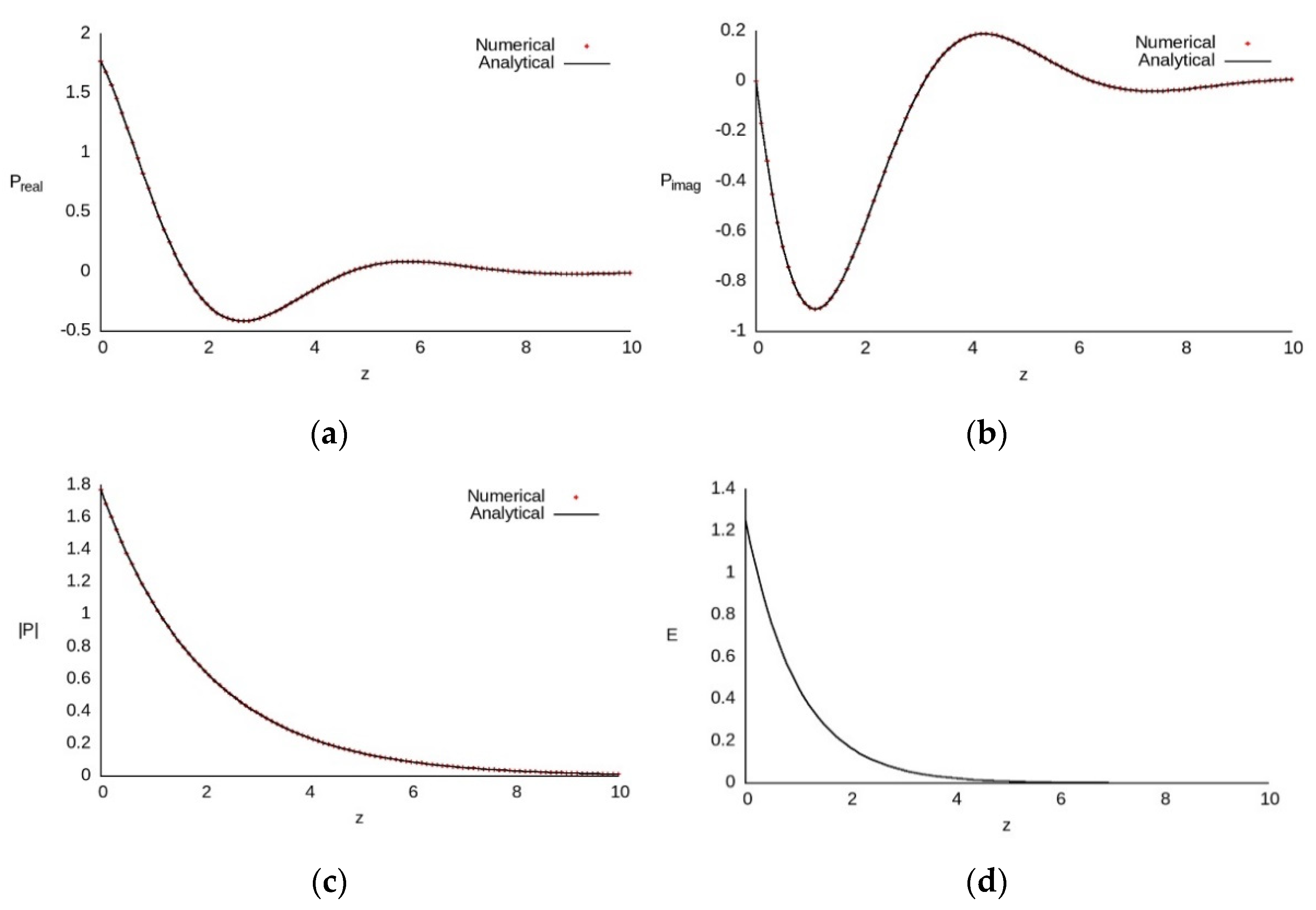
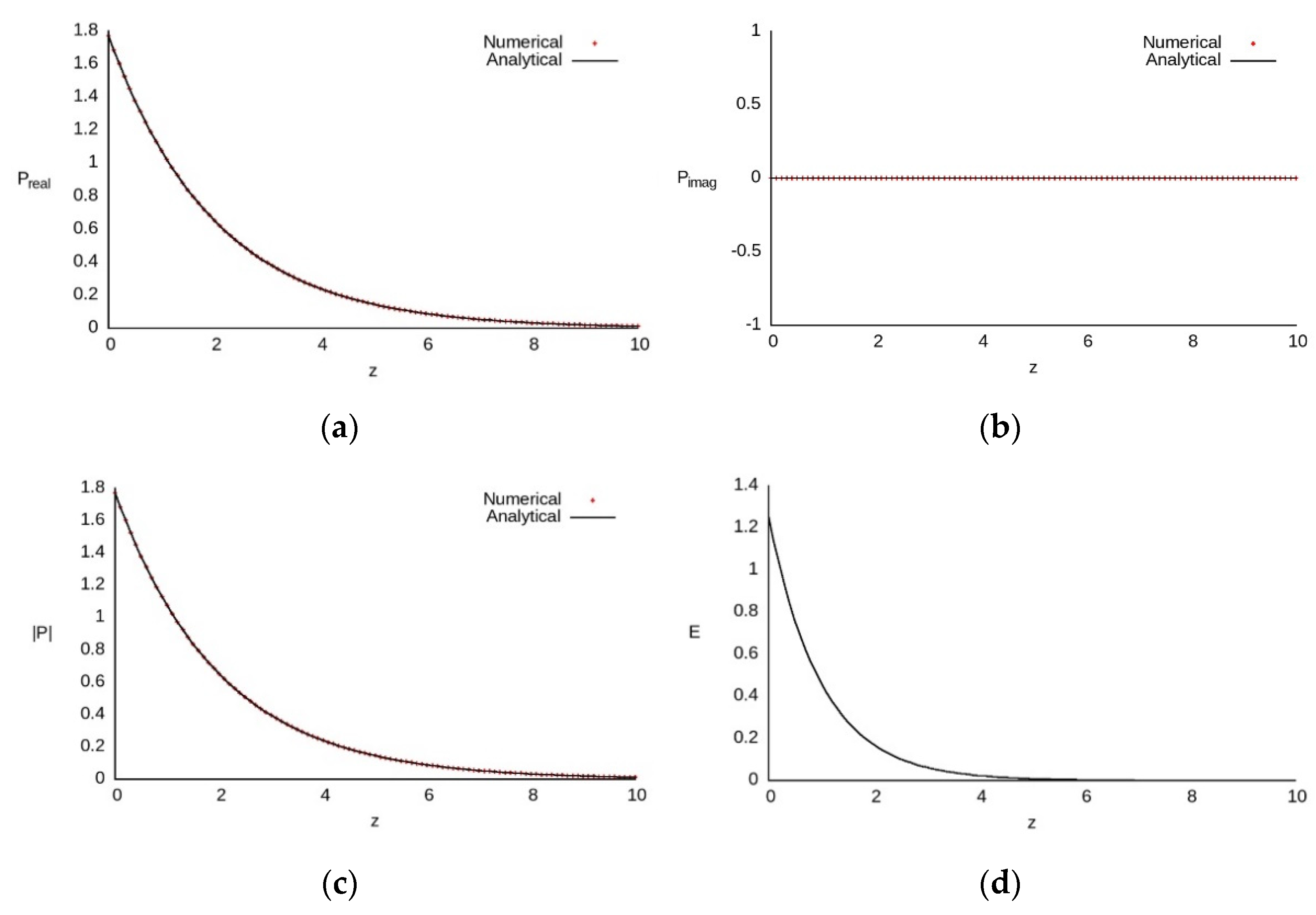
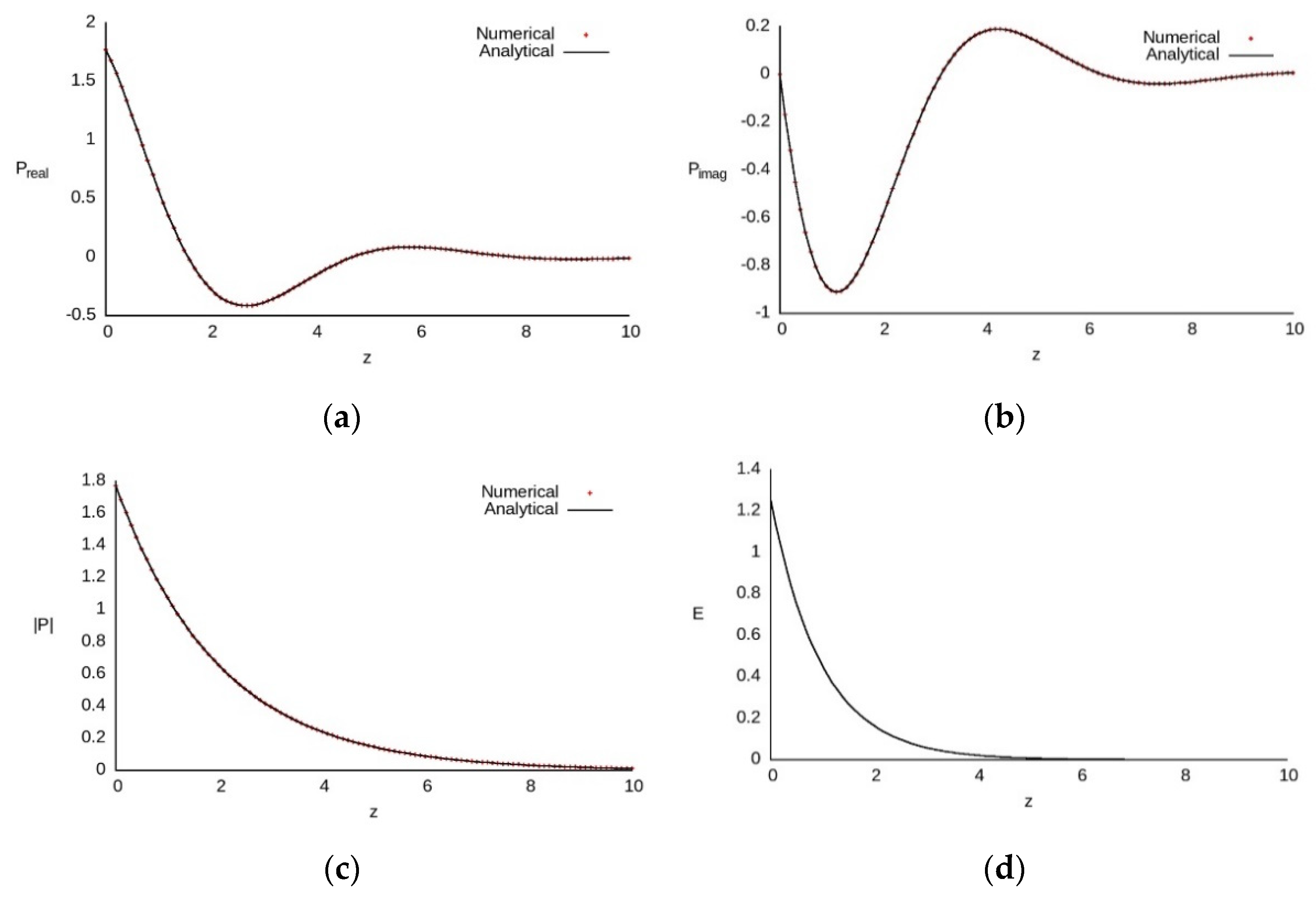
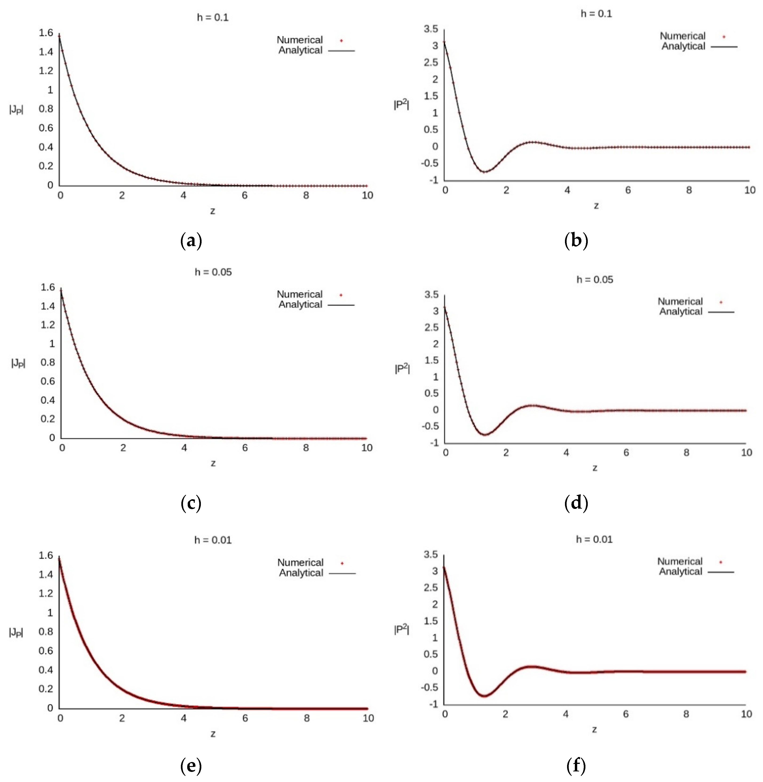
6. Computer Simulation Results

In this section, the computer simulation results are presented to demonstrate the correctness of the numerical method proposed above, and to demonstrate that the conservation laws are valid for the numerical solution. To provide the computations, the following initial distribution of the complex amplitude (2) is stated:

$$\begin{array}{c}{A}_0(t)=e^{-{(t-0.5·L_t)}^2}\end{array},0\le t\le L_t=30,$$

(63)

for which the initial optical pulse’s energy and initial value of the function $P(z)$ are equal to E(0) = 1.25331, P(0) = 1.77, respectively.

With the aim to support the validity of the developed problem’s (1)–(3) invariants, we compared the simulation results with the analytical dependences of the invariants from the z-coordinate for the linear case: $\delta =0,\alpha =0$. Such a comparison is provided in Figure 1, Figure 2, Figure 3, Figure 4, Figure 5, Figure 6 and Figure 7. The values of several parameters are the same for all numerical experiments, $D_2=0.1$, $\nu = {\nu }_{\omega }=0$, while other parameters can have different values.

In Figure 1, Figure 2, Figure 3, Figure 4 and Figure 5, the evolution of the function $P(z,L_t)$ that represents the invariant (4c), its real $P_{real}$ and imaginary $P_{imag}$ parts, and its modulus $\left|P\right|$, and the pulse’s energy $E$ are depicted. The spatial and time mesh steps are equal to $\tau =0.1, h=0.1$, respectively. In these figures, we can observe a very good coincidence between the numerical and analytical results. Note that the pulse energy has a constant value if the optical energy’s absorption is absent (Figure 1). In Figure 2 and Figure 3, we depict a similar comparison for the medium possessing linear absorption under the presence or absence of terms referring to the homogenous shift of the pulse’s phase. We note that parameter $D_{2\omega }$ is equal to zero: $D_{2\omega }=0$.

In Figure 4 and Figure 5, the computer simulation results are shown for parameter $D_{2\omega }=-0.01$. This value results in laser energy absorption at the pulse propagation. We can observe that, for a linear case of propagation (${\delta }_0=0$), the invariant (4c) preserves its value in accordance with the analytical formula (Figure 4). If a medium absorbs laser energy due to the presence of a linear absorption (${\delta }_0\ne 0$), then the invariant changes in accordance with the analytical formula, which depends only on this type of laser energy absorption (Figure 5) and does not depend on parameter $D_{2\omega }$.

In Figure 6, an evolution of the modulus of the function $J_p(z)$, which represents invariant (4a), and the modulus of function $P^2(z,L_t)$, which represents invariant (4b), are depicted for the parameters $D_{2\omega }=-0.01, {\delta }_0=1, n_0=1$. We provided the computation with the mesh step on the time coordinate equal to $\tau =0.01$, and for a sequence of meshes on the spatial coordinate. We can observe a very weak change in the invariants’ evolution at decreasing mesh step $h$, as well as good coincidence for both lines (red and black lines) corresponding to the computer simulation results and analytical formulas.

In Figure 7, an evolution of the modulus of invariants $J_p(z)$ (4a) and $P(z,L_t)$ (4c) are depicted for the computation provided with mesh steps $\tau =0.01, h=0.01$. Its main aim is a demonstration of the invariants’ validity under various relations between the parameters $D_{2\omega } , \nu , {\nu }_{\omega }, {\delta }_0, n_0$, and we wrote them in the figure’s caption. Since, for some sets of the parameters, the computational results exactly coincide, there are therefore not many lines in Figure 7. The main distinction in the parameters’ values between Figure 7a,b and Figure 7c,d contains the value of the linear absorption ${\delta }_0$. In Figure 7a,b, it is equal to zero, while its value is a unit in Figure 7c,d. We stress that, for all parameters’ sets, the invariants change in accordance with the analytical formulas.

For an illustration of the evolution of the problem’s numerical solution, we conclude this section with Figure 8 and Figure 9, where the pulse intensity evolution is demonstrated in 3D view and in (t, z) projection. The parameters for the computations are the following: $D_{2\omega }=-0.01$, $D_2=0.1$, $\nu =0, {\nu }_{\omega }=0$, ${\delta }_0=0$, $n_0=0$; the mesh steps are set as $h=\tau =0.1$. The initial distribution of the complex amplitude (2) is stated in (63). Figure 8 corresponds to a linear case ($\alpha =0, \delta =0$) of the laser pulse propagation. In turn, Figure 9 corresponds to a nonlinear case ($\alpha =1, \delta =0$). The presented results demonstrate that the numerical results obtained using the constructed FDS are correct and in an agreement with the physical sense.

7. Conclusions

In the current study, we proposed one of the possible ways to develop conservation laws (integrals of motion) for the linear and non-linear Ginzburg–Landau equations describing a laser pulse propagation in an optical fiber with an optical amplifier or with attenuation. Using this approach, a few integrals of motion were developed for various relations between the equation’s parameters.

Based on the Crank–Nicolson scheme, the implicit FDS was constructed. The following conservativeness was proven: corresponding theorems with respect to the preservation of the difference analogs of the invariants of the FDS were stated and proved. For conservative nonlinear FDS realization, an iterative process was applied. Presented computer simulation results confirmed the theoretical study.

It should be emphasized that the proposed approach for the derivation of the integrals of motions can be generalized on the 2D and 3D GLEs involving x and y spatial coordinates. In this case, Equation (1) contains the second-order derivatives of these coordinates with similar terms of the second-order derivatives in time. For such a problem, we can introduce additional functions along these coordinates that are similar (5) and write the corresponding invariants using these functions. This is easy to verify directly.

References

1. Ginzburg, V.L.; Landau, L.D. On the theory of superconductivity. In On Superconductivity and Superfluidity; Springer: Berlin/Heidelberg, Germany, 2009. [Google Scholar]
2. Ginzburg, V.L. Superconductivity and superfluidity (what is done and what is not done). Phys.-Uspekh 1997, 40, 407–432. [Google Scholar] [CrossRef]
3. Das, M.P.; Wilson, B.J. Novel superconductivity: From bulk to nano systems. Adv. Nat. Sci.-Nanosci. Nanotechnol. 2015, 6, 013001. [Google Scholar] [CrossRef] [Green Version]
4. Kamenev, A.; Levchenko, A. Keldysh technique and non-linear sigma-model: Basic principles and applications. Adv. Phys. 2009, 58, 197–319. [Google Scholar] [CrossRef]
5. Stoof, H.T.C. Time-dependent Ginzburg-Landau theory for a weak-coupling superconductor. Phys. Rev. B 1993, 47, 7979–7985. [Google Scholar] [CrossRef] [Green Version]
6. Aguirre, C.A.; Martins, Q.S.; Barba-Ortega, J. Superconducting 3D Multi-layer Sample Simulated Via Nonuniform Ginzburg–Landau Parameter. J. Low Temp. Phys. 2021, 202, 360–371. [Google Scholar] [CrossRef]
7. Megne, L.T.; Tabi, C.B.; Kofane, T.C. Modulation instability in nonlinear metamaterials modeled by a cubic-quintic complex Ginzburg-Landau equation beyond the slowly varying envelope approximation. Phys. Rev. E 2020, 102, 042207. [Google Scholar] [CrossRef] [PubMed]
8. Gavish, N.; Kenneth, O.; Keren, A. Ginzburg–Landau model of a Stiffnessometer—A 3D Multi-layer stiffness meter device. Phys. D Nonlinear Phenom. 2021, 415, 132767. [Google Scholar] [CrossRef]
9. Kong, L.; Luo, Y.; Wang, L.; Chen, M.; Zhao, Z. HOC–ADI schemes for two-dimensional Ginzburg–Landau equation in superconductivity. Math. Comput. Simul. 2021, 190, 494–507. [Google Scholar] [CrossRef]
10. El-Nabulsi, R.A. Extended Ginzburg-Landau equations and Abrikrosov vortex and geometric transition from square to rectangular lattice in a magnetic field. Phys. C Supercond. Its Appl. 2021, 581, 1353808. [Google Scholar] [CrossRef]
11. Sadaf, M.; Akram, G.; Dawood, M. An investigation of fractional complex Ginzburg–Landau equation with Kerr law nonlinearity in the sense of conformable, beta and M-truncated derivatives. Opt. Quantum Electron. 2022, 54, 248. [Google Scholar] [CrossRef]
12. Bu, C. The Ginzburg-Landau equation with nonzero Neumann boundary data. Nonlinear Anal. Theory Methods Appl. 1994, 23, 399–404. [Google Scholar] [CrossRef]
13. Chen, X.Y.; Jimbo, S.; Morita, Y. Stabilization of vortices in the Ginzburg-Landau equation with a variable diffusion coefficient. Siam J. Math. Anal. 1998, 29, 903–912. [Google Scholar] [CrossRef]
14. Rajantie, A. Vortices and the Ginzburg-Landau phase transition. Phys. B Condens. Matter 1998, 255, 108–115. [Google Scholar] [CrossRef] [Green Version]
15. Ivey, T.; Lafortune, S. Spectral stability analysis for periodic traveling wave solutions of NLS and CGL perturbations. Phys. D Nonlinear Phenom. 2008, 237, 1750–1772. [Google Scholar] [CrossRef]
16. Liu, C.S. Exact traveling wave solutions for a kind of generalized Ginzburg-Landau equation. Commun. Theor. Phys. 2005, 43, 787–790. [Google Scholar]
17. Mohamadou, A.; Jiotsa, A.K.; Kofane, T.C. Effects of competing first- and second-neighbour couplings on the propagation of unstable patterns in the discrete complex cubic Ginzburg-Landau equation. Phys. Scr. 2005, 72, 281–289. [Google Scholar] [CrossRef]
18. Wazwaz, A.-M. Explicit and implicit solutions for the one-dimensional cubic and quintic complex Ginzburg-Landau equations. Appl. Math. Lett. 2006, 19, 1007–1012. [Google Scholar] [CrossRef] [Green Version]
19. Facao, M.; Carvalho, M.I.; Latas, S.C.; Ferreira, M.F. Control of complex Ginzburg-Landau equation eruptions using intrapulse Raman scattering and corresponding traveling solutions. Phys. Lett. A 2010, 374, 4844–4847. [Google Scholar] [CrossRef] [Green Version]
20. Carvalho, M.I.; Facao, M. Dissipative solitons for generalizations of the cubic complex Ginzburg-Landau equation. Phys. Rev. E 2019, 100, 032222. [Google Scholar] [CrossRef]
21. Balla, P.; Agrawal, G.P. Nonlinear interaction of vector solitons inside birefringent optical fibers. Phys. Rev. A 2018, 98, 023822. [Google Scholar] [CrossRef] [Green Version]
22. Biswas, P.; Gandhi, H.K.; Mishra, V.; Ghosh, S. Propagation and asymmetric behavior of optical pulses through time-dynamic loss-gain-assisted media. Appl. Opt. 2018, 57, 7167–7171. [Google Scholar] [CrossRef] [PubMed] [Green Version]
23. Tafo, J.B.G.; Nana, L.; Kofane, T.C. Effects of nonlinear gradient terms on the defect turbulence regime in weakly dissipative systems. Phys. Rev. E 2017, 96, 022205. [Google Scholar] [CrossRef] [PubMed]
24. Bouzida, A.; Triki, H.; Ullah, M.Z.; Zhou, Q.; Biswas, A.; Belic, M. Chirped optical solitons in nano optical fibers with dual-power law nonlinearity. Optik 2017, 142, 77–81. [Google Scholar] [CrossRef]
25. Li, H.; Yuan, X. Quasi-periodic solution for the complex Ginzburg-Landau equation with continuous spectrum. J. Math. Phys. 2018, 59, 112701. [Google Scholar] [CrossRef]
26. Li, X.; Liu, B. Finite time blow-up and global existence for the nonlocal complex Ginzburg-Landau equation. J. Math. Anal. Appl. 2018, 466, 961–985. [Google Scholar] [CrossRef]
27. Aleksic, B.N.; Uvarova, L.A.; Aleksic, N.B.; Belic, M.R. Cubic quintic Ginzburg Landau equation as a model for resonant interaction of EM field with nonlinear media. Opt. Quantum Electron. 2020, 52, 175. [Google Scholar] [CrossRef] [Green Version]
28. Gao, H.J.; Duan, J.Q. On the initial-value problem for the generalized two-dimensional Ginzburg-Landau equation. J. Math. Anal. Appl. 1997, 216, 536–548. [Google Scholar] [CrossRef]
29. Lu, K.N.; Pan, X.B. Eigenvalue problems of Ginzburg-Landau operator in bounded domains. J. Math. Phys. 1999, 40, 2647–2670. [Google Scholar] [CrossRef] [Green Version]
30. Podivilov, E.; Kalashnikov, V.L. Heavily-chirped solitary pulses in the normal dispersion region: New solutions of the cubic-quintic complex Ginzburg-Landau equation. J. Exp. Theor. Phys. Lett. 2005, 82, 467–471. [Google Scholar] [CrossRef]
31. Shtyrina, O.V.; Yarutkina, I.A.; Skidin, A.S.; Podivilov, E.V.; Fedorukt, M.P. Theoretical analysis of solutions of cubic-quintic Ginzburg-Landau equation with gain saturation. Opt. Express 2019, 27, 6711–6718. [Google Scholar] [CrossRef]
32. Aranson, I.S.; Kramer, L. The world of the complex Ginzburg-Landau equation. Rev. Mod. Phys. 2002, 74, 99–143. [Google Scholar] [CrossRef] [Green Version]
33. Garcia-Morales, V.; Krischer, K. The complex Ginzburg-Landau equation: An introduction. Contemp. Phys. 2012, 53, 79–95. [Google Scholar] [CrossRef]
34. Elcoot, A.E.K. Nonlinear stability of an axial electric field: Effect of interfacial charge relaxation. Appl. Math. Model. 2010, 34, 1965–1983. [Google Scholar] [CrossRef] [Green Version]
35. Agrawal, G.P. Optical pulse propagation in doped fiber amplifiers. Phys. Rev. A 1991, 44, 7493–7501. [Google Scholar] [CrossRef]
36. Agrawal, G.P. Applications of Nonlinear Fiber Optics, 2nd ed.; Academic Press: Rochester, NY, USA, 2008. [Google Scholar] [CrossRef]
37. Arteaga-Sierra, F.R.; Antikainen, A.; Agrawal, G.P. Dynamics of soliton cascades in fiber amplifiers. Opt. Lett. 2016, 41, 5198–5201. [Google Scholar] [CrossRef]
38. van Tartwijk, G.H.M.; Agrawal, G.P. Maxwell-Bloch dynamics and modulation instabilities in fiber lasers and amplifiers. J. Opt. Soc. Am. B Opt. Phys. 1997, 14, 2618–2627. [Google Scholar] [CrossRef]
39. Lugiato, L.A. Transverse nonlinear optics—introduction and review. Chaos Solitons Fractals 1994, 4, 1251–1258. [Google Scholar] [CrossRef]
40. Otsuka, K. Complex dynamics in coupled nonlinear element systems. Int. J. Mod. Phys. B 1991, 5, 1179–1214. [Google Scholar] [CrossRef]
41. Malomed, B.A. Optical Solitons and Vortices in Fractional Media: A Mini-Review of Recent Results. Photonics 2021, 8, 353. [Google Scholar] [CrossRef]
42. Antoine, X.; Bao, W.; Besse, C. Computational methods for the dynamics of the nonlinear Schrödinger/Gross–Pitaevskii equations. Comput. Phys. Commun. 2013, 184, 2621–2633. [Google Scholar] [CrossRef] [Green Version]
43. Sanz-Serna, J.M. Methods for the numerical solution of the nonlinear Schrödinger equation. Math. Comput. 1984, 43, 21–27. [Google Scholar] [CrossRef]
44. Delfour, M.; Fortin, M.; Payr, G. Finite-difference solutions of a non-linear Schrödinger equation. J. Comput. Phys. 1981, 44, 277–288. [Google Scholar] [CrossRef]
45. Wei, Y.; Zhang, X.Q.; Shao, Z.Y.; Gao, J.Q.; Yang, X.F. Multi-symplectic integrator of the generalized KdV-type equation based on the variational principle. Sci. Rep. 2019, 9, 15883. [Google Scholar] [CrossRef]
46. Zhou, M.X.; Kanth, A.S.V.; Aruna, K.; Raghavendar, K.; Rezazadeh, H.; Inc, M.; Aly, A.A. Numerical solutions of time fractional Zakharov-Kuznetsov equation via natural transform decomposition method with nonsingular kernel derivatives. J. Funct. Spaces 2021, 2021, 9884027. [Google Scholar] [CrossRef]
47. Tala-Tebue, E.; Korkmaz, A.; Rezazadeh, H.; Raza, N. New auxiliary equation approach to derive solutions of fractional resonant Schrödinger equation. Anal. Math. Phys. 2021, 11, 167. [Google Scholar] [CrossRef]
48. Samarskii, A.A. The Theory of Difference Schemes, 1st ed.; CRC Press: Boca Raton, FL, USA, 2001. [Google Scholar] [CrossRef]
49. Zhang, F.; Peréz-Ggarcía, V.M.; Vázquez, L. Numerical simulation of nonlinear Schrödinger equation system: A new conservative scheme. Appl. Math. Comput. 1995, 71, 165–177. [Google Scholar] [CrossRef]
50. Li, S.; Vu-Quoc, L. Finite difference calculus invariant structure of a class of algorithms for the nonlinear Klein–Gordon equation. SIAM J. Numer. Anal. 1995, 32, 1839–1875. [Google Scholar] [CrossRef]
51. Gauckler, L. Numerical long-time energy conservation for the nonlinear Schrödinger equation. IMA J. Numer. Anal. 2017, 37, 2067–2090. [Google Scholar] [CrossRef] [Green Version]
52. Ismail, M.S.; Taha, T.R. A linearly implicit conservative scheme for the coupled nonlinear Schrödinger equation. Math. Comput. Simul. 2007, 74, 302–311. [Google Scholar] [CrossRef]
53. Hu, H.; Hu, H. Maximum norm error estimates of fourth-order compact difference scheme for the nonlinear Schrödinger equation involving a quintic term. J. Inequalities Appl. 2018, 1, 180. [Google Scholar] [CrossRef]
54. Wang, T.; Guo, B. Unconditional convergence of two conservative compact difference schemes for non-linear Schrödinger equation in one dimension. Sci. Sin. Math. 2011, 41, 207–233. [Google Scholar] [CrossRef]
55. Trofimov, V.A.; Peskov, N.V. Comparison of finite-difference schemes for the Gross-Pitaevskii equation. Math. Model. Anal. 2009, 14, 109–126. [Google Scholar] [CrossRef]
56. Wang, T.; Jiang, J.; Wang, H.; Xu, W. An efficient and conservative compact finite difference scheme for the coupled Gross–Pitaevskii equations describing spin-1 Bose-Einstein condensate. Appl. Math. Comput. 2018, 323, 164–181. [Google Scholar] [CrossRef]
57. Barletti, L.; Brugnano, L.; Caccia, G.F.; Iavernaro, F. Energy-conserving methods for the nonlinear Schrödinger equation. Appl. Math. Comput. 2018, 318, 3–18. [Google Scholar] [CrossRef]
58. Feng, X.; Liu, H.; Ma, S. Mass- and Energy-Conserved Numerical Schemes for Nonlinear Schrödinger Equations. Commun. Comput. Phys. 2019, 26, 1365–1396. [Google Scholar] [CrossRef] [Green Version]
59. Amiranashvili, S.; Čiegis, R.; Radziunas, M. Numerical methods for a class of generalized nonlinear Schrödinger equations. Kinet. Relat. Models 2015, 8, 215. [Google Scholar] [CrossRef]
60. Trofimov, V.A.; Stepanenko, S.; Razgulin, A. Conservation laws of femtosecond pulse propagation described by generalized nonlinear Schrödinger equation with cubic nonlinearity. Math. Comput. Simul. 2021, 182, 366–396. [Google Scholar] [CrossRef]
61. Varentsova, S.A.; Volkov, A.G.; Trofimov, V.A. The conservative difference scheme for the problem of femtosecond laser pulse propagation through a medium with a cubic nonlinearity. Comput. Math. Math. Phys. 2003, 43, 1644–1656. [Google Scholar]
62. Trofimov, V.; Loginova, M. Conservative Finite-Difference Schemes for Two Nonlinear Schrödinger Equations Describing Frequency Tripling in a Medium with Cubic Nonlinearity: Competition of Invariants. Mathematics 2021, 9, 2716. [Google Scholar] [CrossRef]
63. Paasonen, V.I.; Fedoruk, M.P. Three-level non-iterative high accuracy scheme for Ginzburg—Landau equation. Comput. Technol. 2015, 20, 46–57. [Google Scholar]
64. Du, Q.; Wu, X.N. Numerical solution of the three-dimensional Ginzburg-Landau models using artificial boundary. Siam J. Numer. Anal. 1999, 36, 1482–1506. [Google Scholar] [CrossRef] [Green Version]
65. Borzi, A.; Grossauer, H.; Scherzer, O. Analysis of iterative methods for solving a Ginzburg-Landau equation. Int. J. Comput. Vis. 2005, 64, 203–219. [Google Scholar] [CrossRef] [Green Version]
66. Salete, E.; Vargas, A.M.; García, Á.; Negreanu, M.; Benito, J.J.; Ureña, F. Complex Ginzburg–Landau equation with generalized finite differences. Mathematics 2020, 8, 2248. [Google Scholar] [CrossRef]
67. Takac, P. Invariant 2-tori in the time-dependent Ginzburg-Landau equation. Nonlinearity 1992, 5, 289–321. [Google Scholar] [CrossRef]
68. Du, Q. Discrete gauge invariant approximations of a time dependent Ginzburg-Landau model of superconductivity. Math. Comput. 1998, 67, 965–986. [Google Scholar] [CrossRef] [Green Version]
69. Koma, Y.; Toki, H. Weyl invariant formulation of the flux-tube solution in the dual Ginzburg-Landau theory. Phys. Rev. D 2000, 62, 054027. [Google Scholar] [CrossRef] [Green Version]
70. Lopez, V. Numerical continuation of invariant solutions of the complex Ginzburg-Landau equation. Commun. Nonlinear Sci. Numer. Simul. 2018, 61, 248–270. [Google Scholar] [CrossRef] [Green Version]
71. Gao, H.; Ju, L.; Xie, W. A Stabilized Semi-Implicit Euler Gauge-Invariant Method for the Time-Dependent Ginzburg-Landau Equations. J. Sci. Comput. 2019, 80, 1083–1115. [Google Scholar] [CrossRef]
72. Kulikov, A.; Kulikov, D. Invariant varieties of the periodic boundary value problem of the nonlocal Ginzburg-Landau equation. Math. Methods Appl. Sci. 2021, 44, 11985–11997. [Google Scholar] [CrossRef]
73. Moroz, L.I.; Maslovskaya, A.G. Computer simulation of hysteresis phenomena for ferroelectric switching devices. In Proceedings of the 2020 International Multi-Conference on Industrial Engineering and Modern Technologies (FarEastCon), Vladivostok, Russia, 6–9 October 2020; pp. 1–6. [Google Scholar] [CrossRef]
74. Zhang, M.; Zhang, G.F. Fast iterative solvers for the two-dimensional spatial fractional Ginzburg–Landau equations. Appl. Math. Lett. 2021, 121, 107350. [Google Scholar] [CrossRef]
75. Ding, H.; Yi, Q. The construction of higher-order numerical approximation formula for Riesz derivative and its application to nonlinear fractional differential equations (I). Commun. Nonlinear Sci. Numer. Simul. 2022, 110, 106394. [Google Scholar] [CrossRef]
76. Du, R.; Wang, Y.; Hao, Z. High-dimensional nonlinear Ginzburg–Landau equation with fractional Laplacian: Discretization and simulations. Commun. Nonlinear Sci. Numer. Simul. 2021, 102, 105920. [Google Scholar] [CrossRef]
77. Zhao, Y.L.; Ostermann, A.; Gu, X.M. A low-rank Lie-Trotter splitting approach for nonlinear fractional complex Ginzburg-Landau equations. J. Comput. Phys. 2021, 446, 110652. [Google Scholar] [CrossRef]
Figure 1. The function P ( z , L t ) (4c) evolution: real part (a), imaginary part (b), its modulus (c), and the pulse’s energy (d) obtained via computer simulation (red dotted line) and analytical solution (black solid line) with the parameters D 2 ω = 0 ,     δ 0 = 0 ,     n 0 = 1 .
Mathematics 10 01912 g001
Figure 2. The function P ( z , L t ) (4c) evolution: real part (a), imaginary part (b), its modulus (c), and the pulse’s energy (d) obtained via computer simulation (red dotted line) and analytical solution (black solid line) with the parameters D 2 ω = 0 ,     δ 0 = 1 ,     n 0 = 1 .
Mathematics 10 01912 g002
Figure 3. The function P ( z , L t ) (4c) evolution: real part (a), imaginary part (b), its modulus (c), and the pulse’s energy (d) obtained via computer simulation (red dotted line) and analytical solution (black solid line) with the parameters D 2 ω = 0 ,     δ 0 = 1 ,     n 0 = 0 .
Mathematics 10 01912 g003
Figure 4. The function P ( z , L t ) (4c) evolution: real part (a), imaginary part (b), its modulus (c), and the pulse’s energy (d) obtained via computer simulation (red dotted line) and analytical solution (black solid line) with the parameters D 2 ω = 0.01 ,     δ 0 = 0 ,     n 0 = 1 .
Mathematics 10 01912 g004
Figure 5. The function P ( z , L t ) (4c) evolution: real part (a), imaginary part (b), its modulus (c), and the pulse’s energy (d) obtained via computer simulation (red dotted line) and analytical solution (black solid line) with the parameters D 2 ω = 0.01 ,     δ 0 = 1 ,     n 0 = 1 .
Mathematics 10 01912 g005
Figure 6. Evolution of the modulus of the invariants J p ( z ) (4a) and P 2 ( z , L t ) (4b), computed with parameters D 2 ω = 0.01 ,     δ 0 = 1 ,     n 0 = 1 via computer simulation (red dotted line) and analytically (black solid line) for different values of the following spatial steps: h = 0.1 (a,b), 0.05 (c,d), 0.01 (e,f).
Mathematics 10 01912 g006
Figure 7. Evolution of the modulus of the invariants J p ( z ) (4a) and modulus of the function P ( z , L t ) (4c) computed via computer simulation (red dotted line) and analytically (black solid line) for the following parameters sets: ( D 2 ω ,     ν ,     ν ω , δ 0 ,   n 0 ) = (0, 0.3, 0, 0, 0), (0, 0, 0.05, 0, 0), (0, 0.3, 0.05, 0, 0), (−0.01, 0.3, 0, 0, 0), (−0.01, 0, 0.05, 0, 0), (−0.01, 0.3, 0.05, 0, 0), (−0.01, 0, 0.05, 0, 1) (a,b); (−0.01, 0.3, 0, 1, 0), (−0.01, 0.3, 0.05, 1, 1) (c,d).
Mathematics 10 01912 g007
Figure 8. Evolution of the intensity | A | 2 depicted in 3D view (a), and on the (t,z) plane (b) and computed for the pulse propagation in a linear medium α = 0 ,   δ = 0 .
Mathematics 10 01912 g008
Figure 9. Evolution of the intensity | A | 2 depicted in 3D view (a), and on the (t,z) plane (b) and computed for the pulse propagation in a nonlinear medium α = 1 ,   δ = 0 ; parameters ε 1 = 0.01 ,   ε 2 = 0.001 in the convergence criterion (28).
Mathematics 10 01912 g009
Publisher’s Note: MDPI stays neutral with regard to jurisdictional claims in published maps and institutional affiliations.