Approximate Solution of Nonlinear Time-Fractional PDEs by Laplace Residual Power Series Method

Abstract

Most physical phenomena are formulated in the form of non-linear fractional partial differential equations to better understand the complexity of these phenomena. This article introduces a recent attractive analytic-numeric approach to investigate the approximate solutions for nonlinear time fractional partial differential equations by means of coupling the Laplace transform operator and the fractional Taylor’s formula. The validity and the applicability of the used method are illustrated via solving nonlinear time-fractional Kolmogorov and Rosenau–Hyman models with appropriate initial data. The approximate series solutions for both models are produced in a rapid convergence McLaurin series based upon the limit of the concept with fewer computations and more accuracy. Graphs in two and three dimensions are drawn to detect the effect of time-Caputo fractional derivatives on the behavior of the obtained results to the aforementioned models. Comparative results point out a more accurate approximation of the proposed method compared with existing methods such as the variational iteration method and the homotopy perturbation method. The obtained outcomes revealed that the proposed approach is a simple, applicable, and convenient scheme for solving and understanding a variety of non-linear physical models.

1. Introduction

The subject of fractional calculus is not new. It is a generalization of classical calculus that deals with the ordinary differentiation and integration of arbitrary order. It goes back to Leibniz in a letter to L’Hospital in the late seventeenth century. The main idea of fractional calculus is that natural phenomena modeling is not in integer operators; it is in fractional operators. So, the fractional calculus focuses on behaviors that cannot be modeled by traditional theory [1,2,3,4,5,6,7]. In the past, a lot of prominent contributions were made to the subject of the theory and applications of fractional partial differential equations (FPDEs). These equations are more effectively used to analyze and describe several phenomena in various fields such as mechanical systems, dynamical systems, control theory, mixed convection flows, heat transfer, unification of diffusion, image processing, and wave propagation phenomenon [8,9,10,11,12,13,14,15]. Nevertheless, no method gives an explicit solution for FPDEs due to the intricacies of the fractional calculus that includes these equations. Recently, numerical techniques such as the Adomian decomposition method (ADM), variational iteration method (VIM), reproducing kernel method (RKM), Laplace variational iteration method (LVIM), Laplace Adomian decomposition method (LADM), and residual power series method (RPSM) are used widely to find approximate solutions of many nonlinear fractional differential equations that do not have exact analytic solutions. For more information regarding the methods and numerical techniques for solving fractional differential equations [16,17,18,19,20,21,22]. On the other hand, RPSM has been widely used to find out the solutions to linear and nonlinear issues of fractional differential, and it is used to find out the solution for the system of FPDEs [22]. Additionally, it is used for well-known partial differential equations of fractional order, such as fractional Newell–Whitehead–Segel equation [23], time-fractional Fokker–Planck equations [24], fractional Kundu–Eckhaus and massive Thirring models [25], coupled fractional resonant Schrödinger equation [26], and fuzzy fractional IVPs [27,28,29,30,31,32]. The proposed algorithm is straightforward, accurate, and powerful and creates a series of solutions for different models that occur in applied mathematics without terms of perturbation, discretization, and linearization.

Creating approximation solutions for nonlinear time FPDEs using the aforementioned numeric-analytic methods and others is a significant matter for scholars. Thus, there has become an insistent requirement for efficient semi-analytic methods to construct precise solutions for both linear and nonlinear fractional models. Motivated by this, the primary contribution of this work is to create accurate approximate solutions in a closed-form series for a certain class of nonlinear time FPDEs in light of the time-Caputo fractional derivative sense via extending the application of the Laplace RPSM. This method is proposed and proved by El-Ajou [31] to investigate the exact solitary solutions for a class of nonlinear time-FPDEs. It depends basically on treating the main problem in Laplace space with the help of RPSM, where the unknown coefficients could be found via the concept limit, unlike the RPSM which uses the fractional derivatives in each step to find these coefficients [33]. The proposed method has been successfully employed to produce exact and precise approximate solutions by involving fast convergent power series for emerging realism models in physical phenomena due to its features, which are that it is easy, straightforward, handles directly to various kinds of initial conditions, needs no to linearization or restrictive assumptions, does not need major computational requirements and is performed with less time and more accuracy. More applications, analysis, and advanced techniques used to process and solve linear and non-linear real-life models are found in the references [34,35,36,37,38,39,40,41,42,43,44,45,46,47].

The structure of the article is arranged as follows. In Section 2, essential definitions, properties, and theorems about fractional calculus, Laplace transform, and Laplace fractional expansion (FE) are shown. The methodology of Laplace RPSM for solving nonlinear time-FPDEs is investigated in Section 3. In Section 4, two initial value problems (IVPs) of fractional-order Kolmogorov equation and Rosenau–Hyman equation are solved to show the applicability and accuracy of our approach. Finally, Section 5 is devoted to the conclusions.

2. Basic Concepts and Notations

In this section, we review the essential definitions and theorems of fractional derivatives in the sense of Caputo. Additionally, we revise the primary definitions and theorems related to Laplace transform which will be used mainly in the next section.

Definition 1

(See Ref. [3]). For $𝒶\in {ℝ}^{+}$, the Riemann–Liouville fractional integral operator for a real-valued function $𝒲\left(x,t\right)$ is denoted by ${\mathsf{𝓘}}_t^{𝒶}$ and defined as:

$${\mathsf{𝓘}}_t^{𝒶}\mathcal{W}\left(x,t\right)=\{\begin{array}{ll}\frac{1}{\mathsf{\Gamma }\left(𝒶\right)}\underset{0}{\overset{t}{{\displaystyle \int }}}\frac{\mathcal{W}\left(x,\eta \right)}{{\left(t-\eta \right)}^{1-𝒶}}d\eta , \hfill & 0\le \eta <t,𝒶>0,\hfill \\ \mathcal{W}\left(x,t\right),\hfill & 𝒶=0.\hfill \end{array}$$

Definition 2

(See Ref. [3]). The time fractional derivative of order $𝒶>0$, for the function $\mathcal{W}\left(x,t\right)$ in the Caputo case is denoted by ${\mathfrak{D}}_t^{𝒶}$, and defined as:

$${\mathfrak{D}}_t^{𝒶}\mathcal{W}\left(x,t\right)=\{\begin{array}{ll}{\mathsf{𝓘}}_t^{n-\alpha }\left(D_t^n\mathcal{W}\left(x,t\right)\right),\hfill & 0<n-1<𝒶\le n, \hfill \\ D_t^n\mathcal{W}\left(x,t\right),\hfill & 𝒶=n,\hfill \end{array}$$

where $D_t^n=\frac{{\partial }^n}{\partial t^n}$, and $n\in \mathbb{N}$.

Consequently, for $n-1<𝒶\le n, \beta >-1$ and $t\ge 0$, the operators ${\mathfrak{D}}_t^{𝒶}$ and ${\mathsf{𝓘}}_t^{\alpha }$ satisfy the following properties:

• ${\mathfrak{D}}_t^{𝒶}c=0$,$c\in ℝ$.
• ${\mathfrak{D}}_t^{𝒶}{t}^{\beta }=\frac{\mathsf{\Gamma }\left(\beta +1\right)}{\mathsf{\Gamma }\left(\beta +1-𝒶\right)}{t}^{\beta -𝒶}.$
• ${\mathfrak{D}}_t^{𝒶}{\mathsf{𝓘}}_t^{𝒶}\mathcal{W}\left(x,t\right)=\mathcal{W}\left(x,t\right)$.
• ${\mathsf{𝓘}}_t^{𝒶}{\mathfrak{D}}_t^{𝒶}\mathcal{W}\left(x,t\right)=\mathcal{W}\left(x,t\right)-{\displaystyle \sum }_{j=0}^{n-1}{D}_t^j\left(x,0^{+}\right)\frac{t^j}{j!}$, for$\mathcal{W}\in C^n\left[a,b\right]$, n$-1<𝒶\le n, n\in \mathbb{N} and a,b\in ℝ$.

Definition 3

(See Ref. [31]). Let $\mathcal{W}\left(x,t\right)$ is a piecewise continuous function on $I\times [0,\infty )$ and of exponential order $\delta$. Then, the Laplace transformation of the function $\mathcal{W}\left(x,t\right)$ is denoted and defined as follows:

$$𝝕\left(x,s\right)=ℒ\left[\mathcal{W}\left(x,t\right)\right]≔{{\displaystyle \int }}_0^{\infty }{e}^{-st}\mathcal{W}\left(x,t\right)dt,\hspace{1em}s>\delta ,$$

whereas the inverse Laplace transformation of the function $\mathcal{W}\left(x,s\right)$ is defined as follows:

$$\mathcal{W}\left(x,t\right)={ℒ}^{-1}\left[𝝕\left(x,s\right)\right]≔{{\displaystyle \int }}_{c-i\infty }^{c+i\infty }{e}^{st}𝝕\left(x,s\right)ds, c=Re\left(s\right)>{\delta }_0,$$

where ${\delta }_0$ lies in the right half plane of the absolute convergence of the Laplace integral.

Lemma 1

(See Ref. [31]). Let $\mathcal{W}\left(x,t\right)$ and $\phi \left(x,t\right)$ are piecewise continuous functions on $I\times [0,\infty )$ and of exponential order ${\delta }_1$ and ${\delta }_2$, respectively, where ${\delta }_1<{\delta }_2$. Suppose that $𝝕\left(x,s\right)=ℒ\left[\mathcal{W}\left(x,t\right)\right], \Phi \left(x,s\right)=ℒ\left[\phi \left(x,t\right)\right]$, and $a, b$ are constants. Then, the following properties are satisfied:

• $ℒ\left[a\mathcal{W}\left(x,t\right)+b\phi \left(x,t\right)\right]=a𝝕\left(x,s\right)+b\mathsf{\Phi }\left(x,s\right),x\in I, s>{\delta }_1$.
• ${ℒ}^{-1}\left[a𝝕\left(x,s\right)+b\mathsf{\Phi }\left(x,s\right)\right]=a\mathcal{W}\left(x,t\right)+b\phi \left(x,t\right),x\in I, t\ge 0$.
• $ℒ\left[e^{at}\mathcal{W}\left(x,t\right)\right]=𝝕\left(x,s-a\right),x\in I, s>a+{\delta }_1$.
• $\underset{s\to \infty }{\lim }s𝝕\left(x,s\right)=\mathcal{W}\left(x,0\right), x\in I$.

Lemma 2

(See Ref. [31]). Let $\mathcal{W}\left(x,t\right)$ be a piecewise continuous function on $I\times [0,\infty )$ and of exponential order $\delta$, and $𝝕\left(x,s\right)=ℒ\left[\mathcal{W}\left(x,t\right)\right]$. Then,

• $ℒ\left[\mathsf{𝓘}\mathcal{W}\left(x,t\right)\right]=s^{𝒶-1}𝝕\left(x,s\right), 𝒶>0$
• $ℒ\left[{\mathfrak{D}}_t^{𝒶}\mathcal{W}\left(x,t\right) \right]=s^{𝒶}𝝕\left(x,s\right)-{\displaystyle \sum }_{k=0}^{n-1}{s}^{𝒶-k-1}{D}_t^k\mathcal{W}\left(x,0\right),n-1<𝒶\le n$
• $ℒ\left[{\mathfrak{D}}_t^{j𝒶}\mathcal{W}\left(x,t\right) \right]=s^{j𝒶}𝝕\left(x,s\right)-{\displaystyle \sum }_{k=0}^{j-1}{s}^{\left(j-k\right)𝒶-1}{D}_t^{k𝒶}\mathcal{W}\left(x,0\right),0<𝒶\le 1,$where ${\mathfrak{D}}_t^{j𝒶}={\mathfrak{D}}_t^{𝒶}·{\mathfrak{D}}_t^{𝒶}\cdots {\mathfrak{D}}_t^{𝒶}\left(j-times\right)$

Theorem 1

(See Ref. [31]). Let $\mathcal{W}\left(x,t\right)$ be a piecewise continuous function on $I\times [0,\infty )$ and of exponential order $\delta$. Suppose that the function $𝝕\left(x,s\right)=ℒ\left[\mathcal{W}\left(x,t\right)\right]$ has the following fractional expansion:

$$𝝕\left(x,s\right)={\displaystyle \sum }_{n=0}^{\infty }\frac{h_n\left(x\right)}{s^{n\alpha +1}}, x\in I, s>\delta , 0<𝒶\le 1.$$

Then, $h_n\left(x\right)={\mathfrak{D}}_t^{n𝒶}\mathcal{W}\left(x,0\right)$.

Remark 1.

The inverseLaplace transformation $\mathcal{W}\left(x,t\right)={ℒ}^{-1}\left[𝝕\left(x,s\right)\right]$in Theorem 1 is in the following form:

$$\mathcal{W}\left(x,t\right)={\displaystyle \sum }_{n=0}^{\infty }{\mathfrak{D}}_t^{n𝒶}\mathcal{W}\left(x,0\right)\frac{t^{n𝒶}}{\mathsf{\Gamma }\left(n𝒶+1\right)}, 0< \alpha \le 1,t>0.$$

Theorem 2

(See Ref. [31]). Let $\mathcal{W}\left(x,t\right)$ be a piecewise continuous function on $I\times [0,\infty )$ and of exponential order $\delta$ and $𝝕\left(x,s\right)=ℒ\left[\mathcal{W}\left(x,t\right)\right]$ can be represented as the fractional expansion in Theorem 1. If $\left|sℒ\left[{\mathfrak{D}}_t^{\left(n+1\right)a}\mathcal{W}\left(x,t\right) \right]\right|\le M\left(x\right)$, on $I\times (\delta ,\gamma ]$ where $0<𝒶\le 1$, then the remainder $R_n\left(x,s\right)$ of the FE in Theorem 1 satisfies the following inequality:

$$\left|R_n\left(x,s\right)\right|\le \frac{M\left(x\right)}{s^{1+\left(n+1\right)𝒶}}, x\in I, \delta <s\le \gamma .$$

Theorem 3.

If $𝒶\in \left(0,1\right)$, $\Vert {\mathcal{W}}_{k+1}\left(x,t\right)\Vert \le 𝒶\Vert {\mathcal{W}}_k\left(x,t\right)\Vert$gives $\forall k\in N$and $0<t<\mathrm{T}<1$, then the series of numerical solutions converges to an exact solution [35].

Proof. 

We notice that $\forall 0<t<\mathrm{T}<1$,

$$\parallel \mathcal{W}\left(x,t\right)-{\mathcal{W}}_k\left(x,t\right)\parallel =\parallel {\displaystyle \sum }_{m=k+1}^{\infty }{\mathcal{W}}_m\left(x,t\right)\parallel \le {\displaystyle \sum }_{m=k+1}^{\infty }\parallel {\mathcal{W}}_m(x,t\parallel )\le \parallel ℊ\left(\eta \right)\parallel \parallel {\displaystyle \sum }_{m=k+1}^{\infty }{C}^m\parallel =\frac{{𝒶}^{k+1}}{1-𝒶}\parallel ℊ\left(\eta \right)\parallel \to 0 as k\to \infty .$$

 □

3. Methodology of Laplace RPSM

In this section, we clarify the principle of the Laplace RPSM algorithm to solve nonlinear time fractional PDEs. Our strategy to use the proposed scheme depends on coupling the Laplace transform operator and fractional RPSM. More specifically, consider the following initial value problem of nonlinear time fractional PDEs:

$$\{\begin{array}{c}{\mathfrak{D}}_t^{𝒶}W\left(x,t\right)=N_x\left[\mathcal{W}\left(x,t\right)\right],\\ W\left(x,0\right)=f\left(x\right),\end{array}$$

(1)

where $N_x$ is a nonlinear operator relative to $x$ of degree $r$, $x\in I$, $t\ge 0$, ${\mathfrak{D}}_t^{𝒶}$ refers to $𝒶$-th Caputo fractional derivative for $𝒶\in \left(0,1\right]$, and $\mathcal{W}\left(x,t\right)$ is an unknown function to be determined.

To construct the approximate solution of (1) by using the Laplace RPSM, one can perform the following procedure:

Step A: Apply the Laplace transform on both sides of (1), and utilizing the initial data of (1), as well as depending on Lemma 2, part (2), we get:

$$\begin{gathered} 𝝕\left(x,s\right)=\frac{f\left(x\right)}{s}-\frac{1}{s^{𝒶}}ℒ\left\{N_x\left[\mathcal{W}\left(x,t\right)\right]\right\}, \\ \mathrm{where}𝝕\left(x,s\right)=ℒ\left[\mathcal{W}\left(x,t\right)\right]\left(s\right), s>\delta . \end{gathered}$$

(2)

Step B: According to Theorem 1, we assume that the approximate solution of the Laplace Equation (2) takes the following fractional expansion:

$$𝝕\left(x,s\right)=\frac{f\left(x\right)}{s}+{\displaystyle \sum }_{n=1}^{\infty }\frac{h_n\left(x\right)}{s^{n𝒶+1}}, x\in I, s>\delta \ge 0,$$

(3)

and the k-th Laplace series solution takes the following form:

$${𝝕}_k\left(x,s\right)=\frac{f\left(x\right)}{s}+{\displaystyle \sum }_{n=1}^k\frac{h_n\left(x\right)}{s^{n𝒶+1}}, x\in I, s>\delta \ge 0.$$

(4)

Step C: We define the k-th Laplace fractional residual function of (2) as

$$ℒ\left(Re{s}_{{𝝕}_k}\left(x,s\right)\right)={𝝕}_k\left(x,s\right)-\frac{f\left(x\right)}{s}+\frac{1}{s^{𝒶}}ℒ\left\{N_x\left[\mathcal{W}\left(x,t\right)\right]\right\},$$

(5)

and the Laplace residual function of (2) are defined as:

$$\underset{k\to \infty }{\lim }ℒ\left(Re{s}_{{𝝕}_k}\left(x,s\right)\right)=ℒ\left(Re{s}_{𝝕}\left(x,s\right)\right)=𝝕\left(x,s\right)-\frac{f\left(x\right)}{s}+\frac{1}{s^{𝒶}}ℒ\left\{N_x\left[\mathcal{W}\left(x,t\right)\right]\right\}.$$

(6)

As in [31,32,33], some useful facts of Laplace residual function which are essential in finding the approximate solution are listed as follows:

• $\underset{k\to \infty }{\lim }ℒ\left(Re{s}_{{𝝕}_k}\left(x,s\right)\right)=ℒ\left(Re{s}_{𝝕}\left(x,s\right)\right)$, for $x\in I,s>\delta \ge 0$.
• $ℒ\left(Re{s}_{𝝕}\left(x,s\right)\right)=0$, for $x\in I,s>\delta \ge 0$.
• $\underset{s\to \infty }{\lim }{s}^{k𝒶+1}ℒ\left(Re{s}_{{𝝕}_k}\left(x,s\right)\right)=0$, for $x\in I,s>\delta \ge 0$, and $k=1,2,3,\dots$

Step D: Substitute the k-th Laplace series solution (4) into the k-th Laplace fractional residual function of (5).

Step E: The unknown coefficients $h_k\left(x\right)$, for $k=1,2,3,\dots$, could be founded by solving the system $\underset{s\to \infty }{\lim }{s}^{k𝒶+1}ℒ\left(Re{s}_{{𝝕}_k}\left(x,s\right)\right)=0$. Then, we collect the obtained coefficients in terms of fractional expansion series (4) ${𝝕}_k\left(x,s\right)$.

Step F: Running the inverse Laplace transform operator on both sides of the obtained Laplace series solution to get the approximate solution ${\mathcal{W}}_k\left(x,t\right)$, of the main Equation (1).

4. Numerical Examples

In this section, the superiority, efficiency, and applicability of the Laplace RPSM are demonstrated by testing two non-linear time fraction IVPs. It is worth mention here that all numerical computations and symbolic have been carried out using MATHEMATICA 12 software package.

Example 1.

Consider the following nonlinear time-fractional Kolmogorov IVP:

$$\{\begin{array}{c}{\mathfrak{D}}_t^{𝒶}W\left(x,t\right)-\left(x+1\right){\mathfrak{D}}_{x}W\left(x,t\right)-x^2{e}^t{\mathfrak{D}}_x^{2}W\left(x,t\right)=0,\\ W\left(x,0\right)=x+1,\end{array}$$

(7)

where $0<𝒶\le 1$, and $\left(x,t\right)\in \left[0,1\right]\times ℝ$. The exact solutions for standard case $𝒶=1$, is given as $\mathcal{W}\left(x,t\right)=\left(x+1\right)e^t$.

By applying the Laplace transform operator on the both sides of time-fractional Kolmogorov equation of (7) and using part 2 in Lemma 2 and the initial data-space of $\left(7\right)$, we get the following Laplace fractional equation:

$$𝝕\left(x,s\right)=\frac{x+1}{s}+\frac{x+1}{s^{𝒶}}{D}_x𝝕\left(x,s\right)+\frac{x^2}{s^{𝒶}}ℒ\left\{{ℒ}^{-1}\left\{\frac{1}{s-1}\right\}{D}_x^2{ℒ}^{-1}\left\{𝝕\right\}\right\},$$

(8)

where $𝝕\left(x,s\right)=ℒ\left[\mathcal{W}\left(x,t\right)\right].$

Considering the last discussion, the k-th Laplace series, ${𝝕}_k\left(x,s\right)$ for (8) is expressed as the form:

$${𝝕}_k\left(x,s\right)=\frac{x+1}{s}+{\displaystyle \sum }_{n=1}^k\frac{h_n\left(x\right)}{s^{n𝒶+1}}.$$

(9)

In addition, we define the k-th Laplace residual function of (8) as

$$ℒ\left(Re{s}_{{𝝕}_k}\left(x,s\right)\right)={\displaystyle \sum }_{n=1}^k\frac{h_n\left(x\right)}{s^{n𝒶+1}}-\frac{x+1}{s^{𝒶}}{D}_x\left(\frac{x+1}{s}+{\displaystyle \sum }_{n=1}^k\frac{h_n\left(x\right)}{s^{n𝒶+1}}\right)-\frac{x^2}{s^{𝒶}}ℒ\left\{{ℒ}^{-1}\left\{\frac{1}{s-1}\right\}{D}_x^2{ℒ}^{-1}\left\{\frac{x+1}{s}+{\displaystyle \sum }_{n=1}^k\frac{h_n\left(x\right)}{s^{n𝒶+1}}\right\}\right\}.$$

(10)

For $k=1$, in (10), we get the 1-st Laplace residual function as

$$\begin{gathered} ℒ\left(Re{s}_{{𝝕}_1}\left(x,s\right)\right)=\frac{h_1\left(x\right)}{s^{𝒶+1}}-\frac{x+1}{s^{𝒶}}{D}_x\left(\frac{x+1}{s}+\frac{h_1\left(x\right)}{s^{𝒶+1}}\right)-\frac{x^2}{s^{𝒶}}ℒ\left\{{ℒ}^{-1}\left\{\frac{1}{s-1}\right\}{D}_x^2{ℒ}^{-1}\left\{\frac{x+1}{s}+\frac{h_1\left(x\right)}{s^{𝒶+1}}\right\}\right\} \\ =\frac{h_1\left(x\right)}{s^{𝒶+1}}-\frac{x+1}{s^{𝒶}}\left(\frac{1}{s}+\frac{h_1^{\prime }\left(x\right)}{s^{𝒶+1}}\right)-\frac{x^2{h}_1^{″}\left(x\right)}{{\left(s-1\right)}^{2𝒶+1}{s}^{𝒶}}. \end{gathered}$$

(11)

Next, multiply both sides of (11) by $s^{𝒶+1},$ and then solve the system $\underset{s\to \infty }{lim}{s}^{𝒶+1}ℒ\left(Re{s}_{{𝝕}_1}\left(x,s\right)\right)=0$, and we get: $h_1\left(x\right)=x+1$. So, the 1-st Laplace series solution of (8) could be written as: ${𝝕}_1\left(x,s\right)=\frac{x+1}{s}+\frac{x+1}{s^{𝒶+1}}$.

For $k=2$, in (10), then the 2-nd Laplace residual function can be expressed as

$$\begin{array}{cc}ℒ({Res}_{{𝝕}_2}(x,s))& =\frac{x+1}{s^{𝒶+1}}+\frac{h_2(x)}{s^{2𝒶+1}}-\frac{x+1}{s^{𝒶}}{D}_x(\frac{x+1}{s}+\frac{x+1}{s^{𝒶+1}}+\frac{h_2(x)}{s^{2𝒶+1}})\hfill \\ & -\frac{x^2}{s^{𝒶}}ℒ\left\{{ℒ}^{-1}\right\{\frac{1}{s-1}\left\}{D}_x^2{ℒ}^{-1}\right\{\frac{x+1}{s}+\frac{x+1}{s^{𝒶+1}}+\frac{h_2(x)}{s^{2𝒶+1}}\left\}\right\}\hfill \\ & =\frac{x+1}{s^{𝒶+1}}+\frac{h_2(x)}{s^{2𝒶+1}}-\frac{x+1}{s^{𝒶}}(\frac{1}{s}+\frac{1}{s^{𝒶+1}}+\frac{h_2^{\prime }(x)}{s^{2𝒶+1}})-\frac{x^2{h}_2^{″}(x)}{(s-1{)}^{2𝒶+1}{s}^{𝒶}}\hfill \end{array}$$

(12)

After that, we multiply the result of Equation (12) by the factor $s^{2𝒶+1}$ to get the following equation:

$$s^{2𝒶+1}ℒ\left(Re{s}_{{𝝕}_2}\left(x,s\right)\right)=h_2\left(x\right)-x-1-\frac{\left(x+1\right)h_2^{\prime }\left(x\right)}{s^{𝒶}}-\frac{x^2{h}_2^{″}\left(x\right)}{{\left(s-1\right)}^{2𝒶+1}{s}^{1-𝒶}}.$$

(13)

By solving $\underset{s\to \infty }{lim}{s}^{2𝒶+1}ℒ\left(Re{s}_{{𝝕}_2}\left(x,s\right)\right)=0$, yields that:$h_2\left(x\right)=x+1$. So, the 2-nd Laplace series solution of (8) could be written as: ${𝝕}_2\left(x,s\right)=\frac{x+1}{s}+\frac{x+1}{s^{𝒶+1}}+\frac{x+1}{s^{2𝒶+1}}$.

Similarly, for $k=3$, we have

$$\begin{array}{cc}{s}^{3𝒶+1}ℒ\left({Res}_{{𝝕}_3}(x,s)\right)& \\ & =s^{3𝒶+1}(\frac{x+1}{s^{𝒶+1}}+\frac{x+1}{s^{2𝒶+1}}+\frac{h_3(x)}{s^{3𝒶+1}}\hfill \\ & -\frac{x+1}{s^{𝒶}}{D}_x(\frac{x+1}{s}+\frac{x+1}{s^{𝒶+1}}+\frac{x+1}{s^{2𝒶+1}}+\frac{h_3(x)}{s^{3𝒶+1}})\hfill \\ & -\frac{x^2}{s^{𝒶}}ℒ\left\{{ℒ}^{-1}\right\{\frac{1}{s-1}\left\}{D}_x^2{ℒ}^{-1}\right\{\frac{x+1}{s}+\frac{x+1}{s^{𝒶+1}}+\frac{x+1}{s^{2𝒶+1}}+\frac{h_3(x)}{s^{3𝒶+1}}\left\}\right\})\hfill \\ & =h_3(x)-(x+1)-\frac{(x+1)h_2^{\prime }(x)}{s^{𝒶}}-\frac{x^2{h}_3^{″}(x)}{{(s-1)}^{3a+1}{s}^{1-2a},}\hfill \end{array}$$

(14)

and by solving $\underset{s\to \infty }{lim}{s}^{3𝒶+1}ℒ\left(Re{s}_{{𝝕}_3}\left(x,s\right)\right)=0$, one can obtain that $h_3\left(x\right)=x+1$. So, the $3-rd$ Laplace series solution of (8) could be written as: ${𝝕}_3\left(x,s\right)=\frac{x+1}{s}+\frac{x+1}{s^{𝒶+1}}+\frac{x+1}{s^{2𝒶+1}}+\frac{x+1}{s^{3𝒶+1}}$.

Processing the previous steps for an arbitrary $k$, and using the fact $\underset{s\to \infty }{lim}{s}^{k𝒶+1}ℒ\left(Re{s}_{{𝝕}_k}\left(x,s\right)\right)=0$, one can obtain that: $h_k\left(x\right)=x+1, for k=4,5,\dots$. Thus, the k-th Laplace series solution of (8) could be reformulated by the following fractional expansion:

$${𝝕}_k\left(x,s\right)=\left(\frac{1}{s}+\frac{1}{s^{𝒶+1}}+\frac{1}{s^{2𝒶+1}}+\frac{1}{s^{3𝒶+1}}+\dots +\frac{1}{s^{k𝒶+1}}\right)={\displaystyle \sum }_{n=0}^k\frac{x+1}{s^{n𝒶+1}}.$$

(15)

Lastly, we apply the inverse Laplace transform for the obtained expansion (15) to conclude that the k-th approximate solution of the nonlinear time-fractional Kolmogorov IVP (7) has the form:

$${\mathcal{W}}_k\left(x,t\right)=\left(x+1\right){\displaystyle \sum }_{n=0}^k\frac{t^{n𝒶}}{\mathsf{\Gamma }\left(n𝒶+1\right)},$$

(16)

when $k\to \infty$ and by substituting $𝒶=1$ in (16), we get the Maclaurin series expansion of the closed form $\mathcal{W}\left(x,t\right)=\left(x+1\right)e^t$, which is fully in agreement with the exact solution.

Numerical results of the 10-th approximate solutions for the nonlinear time-fractional Kolmogorov IVP (7) are computed and summarized in Table 1 at fixed values of the variable $\mathrm{x}$, and some selected grid points in $\left[0,1\right]$ with step size of $0.25$, and different values of fractional order $𝒶$’s such that $𝒶\in \left\{1,0.95,0.85,0.75, 0.65\right\}$. From the table, it can be found that the present method provides us with an accurate approximate solution, which is in good agreement with each other for all values of $t$ in $\left[0,1\right]$, especially when approaching the initial values. Further, numerical comparisons are performed in Table 2 to validate the accuracy of our approach by establishing the recurrence errors $|{\mathcal{W}}_8\left(x,t\right)-{\mathcal{W}}_7\left(x,t\right)|$ for the obtained approximate solution of IVP (7) at various values of $𝒶$.

Table 1. Results of the 10-th approximate solution at different values of $𝒶$ for Example 1.

$\mathit{x}$	${\mathit{t}}_{\mathit{i}}$	$𝒶=1$	$𝒶=0.95$	$𝒶=0.85$	$𝒶=0.75$	$𝒶=0.65$
$0$	$0.0$	$1.00$	$1.00$	$1.00$	$1.00$	$1.00$
	$0.25$	$1.2840254167$	$1.3168989383$	$1.3960863710$	$1.4990355063$	$1.6365268759$
	$0.50$	$1.6487212707$	$1.7072557012$	$1.8456231911$	$2.0217199431$	$2.2527959051$
	$0.75$	$2.1170000155$	$2.2042026866$	$2.4091674423$	$2.6683879567$	$3.0068075604$
	$1.0$	$2.7182818011$	$2.8399806687$	$3.1254929139$	$3.4858483992$	$3.9554385524$
$0.5$	$0.0$	$1.00$	$1.00$	$1.00$	$1.00$	$1.00$
	$0.25$	$1.9260381250$	$1.9753484075$	$2.0941295565$	$2.2485532594$	$2.4547903138$
	$0.50$	$2.4730819060$	$2.5608835519$	$2.7684347867$	$3.0325799147$	$3.3791938577$
	$0.75$	$3.1755000232$	$3.3063040300$	$3.6137511635$	$4.0025819351$	$4.5102113406$
	$1.0$	$4.0774227017$	$4.2599710030$	$4.6882393708$	$5.2287725988$	$5.9331578286$

Table 2. The recurrence errors $|{\mathcal{W}}_8\left(x,t\right)-{\mathcal{W}}_7\left(x,t\right)|$ of the tenth approximate solution for Example 1.

${\mathit{t}}_{\mathit{i}}$	$𝒶=0.75$	$𝒶=0.85$	$𝒶=0.95$	$𝒶=1.00$
$0.16$	$2.3301689\times {10}^{-8}$	$1.1468189\times {10}^{-9}$	$5.1702642\times {10}^{-11}$	$1.0651924\times {10}^{-11}$
$0.32$	$1.4913081\times {10}^{-6}$	$1.2779060\times {10}^{-7}$	$1.0030869\times {10}^{-8}$	$2.7269635\times {10}^{-9}$
$0.48$	$1.6986931\times {10}^{-5}$	$2.0133509\times {10}^{-6}$	$2.1859095\times {10}^{-7}$	$6.9889089\times {10}^{-8}$
$0.64$	$9.5443717\times {10}^{-5}$	$1.4239767\times {10}^{-5}$	$1.9461063\times {10}^{-6}$	$6.9810262\times {10}^{-7}$
$0.80$	$3.6408889\times {10}^{-4}$	$6.4936813\times {10}^{-5}$	$1.0609201\times {10}^{-5}$	$4.1610159\times {10}^{-6}$
$0.80$	$1.0871636\times {10}^{-3}$	$2.2434864\times {10}^{-4}$	$4.2409205\times {10}^{-4}$	$1.7891607\times {10}^{-5}$

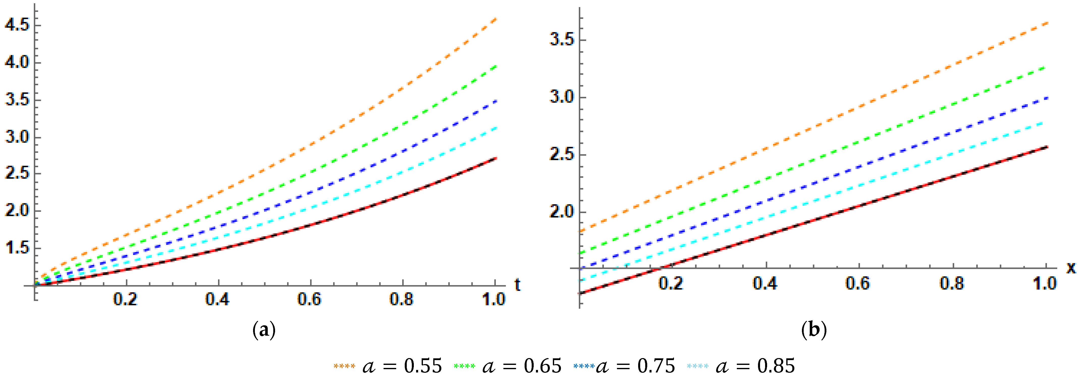
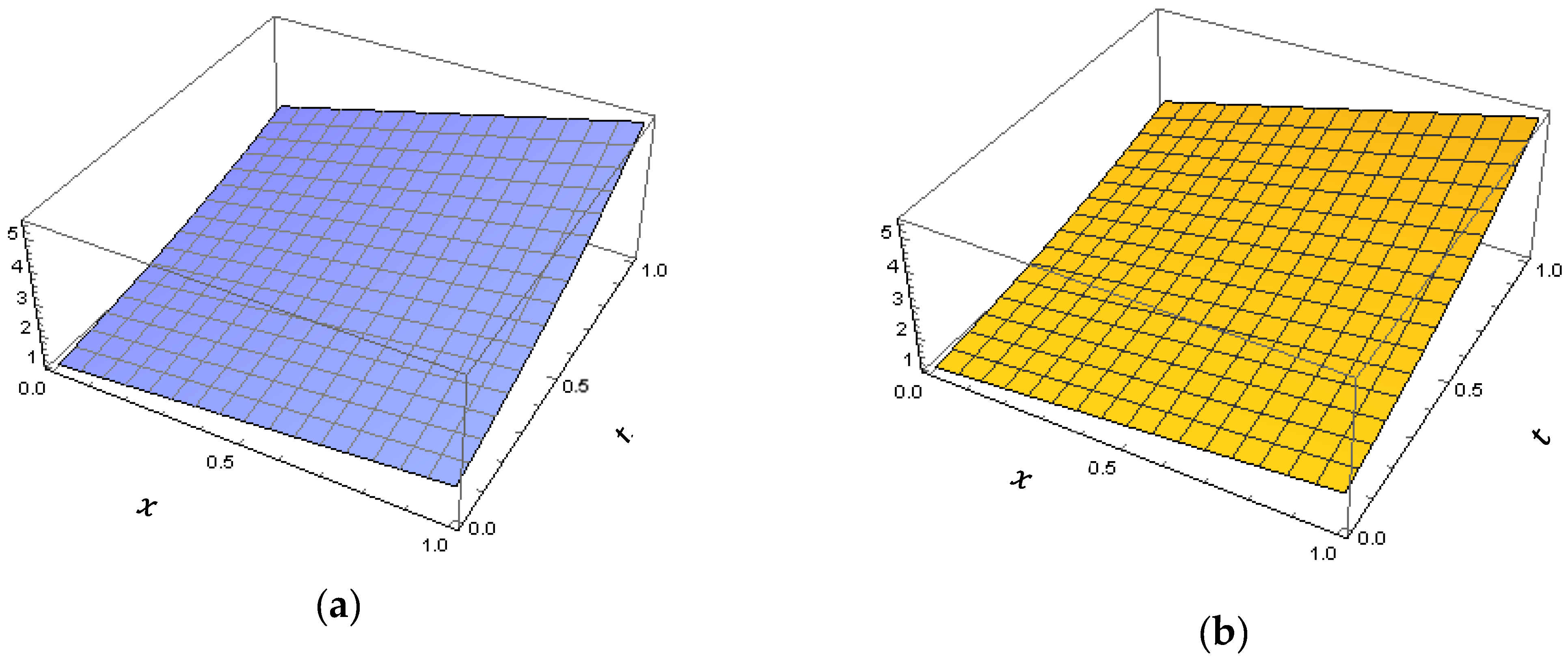
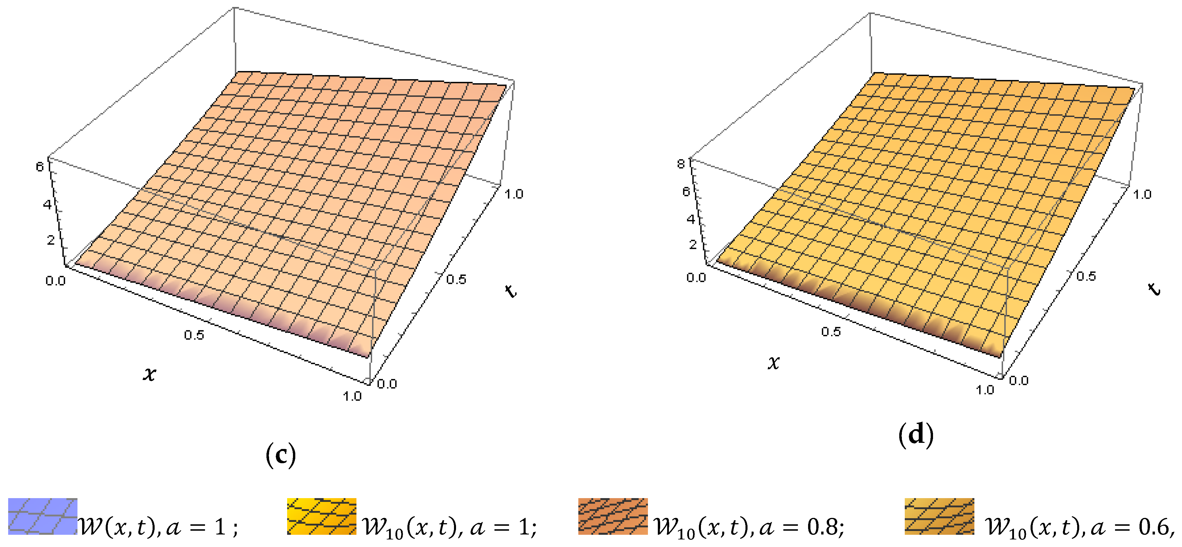
Figure 1 shows the graphs of the exact and the tenth approximate curves solutions for the nonlinear time-fractional Kolmogorov IVP (7) at various $𝒶$ values. Obviously, one can see that the obtained approximate solutions for different values of fractional order simulate the solution for the classical case. Additionally, the exact and approximate solutions match at $𝒶=1$, and this confirms the effectiveness and performance of our approach. While Figure 2 demonstrates the comparison of the geometric behavior between the exact solution and the obtained 10-th approximate solution to the nonlinear time-fractional Kolmogorov IVP (7) at various $𝒶$ values for $\left(x,t\right)\in {\left[0,1\right]}^2$. From these 3D surface plots, we see that the solution behaviors for different Caputo fractional derivatives on their domain are in close agreement with each other, particularly for classical derivative. Moreover, the total calculation cost comparison of the given figures in Example 1 is reported in Table 3.

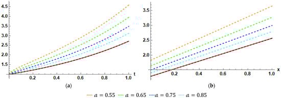
Figure 1. (a) Plots of Exact $\mathcal{W}\left(x,t\right)$ and ${\mathcal{W}}_{10}\left(x,t\right)$ at $x=0$ and with various $𝒶$ values of IVP (7). (b) Plots of Exact $\mathcal{W}\left(x,t\right)$ and ${\mathcal{W}}_{10}\left(x,t\right)$ at $t=0$ and with various $𝒶$ values of IVP (7).

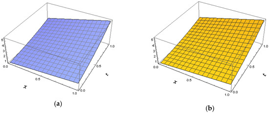
Figure 2. 3D Surface Plots of Exact solution $\mathcal{W}\left(x,t\right)$, and the 10-th approximate solution ${\mathcal{W}}_{10}\left(x,t\right)$, for IVP (7), with $t\in \left[0,1\right]$, and $x\in \left[0,1\right]$, at various values of $𝒶$.

Table 3. Total computational cost for the obtained figures in Example 1.

ID		Image Size (KB)	Maximum Memory (MB)	Tracing Time (s)	Total Cost $(\mathbf{MB}\times \mathbf{S})$
Figure 1	a	$11.5$	$48$	$4.4$	$211.2$
	b	$11.2$	$48$	$4.2$	$201.6$
Figure 2	a	$30.6$	$49$	$4.5$	$220.5$
	b	$34.7$	$50$	$4.4$	$220.0$
	c	$37.4$	$54$	$5.0$	$270.0$
	d	$36.2$	$51$	$4.5$	$229.5$

Example 2.

Consider the following nonlinear time-fractional Rosenau–Hyman IVP:

$$\{\begin{array}{c}{\mathfrak{D}}_t^{𝒶}W-W{D}_x^{3}W-W{D}_{x}W-3D_{x}W{D}_x^{2}W=0,\\ W\left(x,0\right)=-\frac{8c}{3}{\cos }^2\frac{x}{4},\end{array}$$

(17)

where $0<𝒶\le 1$, and $\left(x,t\right)\in \left[0,1\right]\times ℝ$. The exact solutions for standard case $𝒶=1$, is $\mathcal{W}\left(x,t\right)=-\frac{8c}{3}{\cos }^2\left(\frac{x-ct}{4}\right)$.

According to the Laplace RPSM, we firstly operate the Laplace transform to nonlinear time-fractional Rosenau–Hyman of (17), and using the initial data-space of (17), we get:

$$𝝕\left(x,s\right)=\frac{8c}{3s}{\cos }^2\frac{x}{4}+\frac{1}{s^{𝒶}}ℒ\left\{{ℒ}^{-1}\left\{𝝕\right\}{D}_x^3{ℒ}^{-1}\left\{𝝕\right\}\right\}+\frac{1}{s^{𝒶}}ℒ\left\{{ℒ}^{-1}\left\{𝝕\right\}{D}_x{ℒ}^{-1}\left\{𝝕\right\}\right\}+\frac{3}{s^{𝒶}}ℒ\left\{D_x{ℒ}^{-1}\left\{𝝕\right\}{D}_x^2{ℒ}^{-1}\left\{𝝕\right\}\right\}.$$

(18)

The k-th proposed Laplace series solution of the Laplace Equation (18) will be in the form:

$${𝝕}_k\left(x,s\right)=-\frac{8c}{3s}{\cos }^2\frac{x}{4}+{\displaystyle \sum }_{n=1}^k\frac{h_n\left(x\right)}{s^{n𝒶+1}}.$$

(19)

Therefore, the k-th Laplace residual function of (18) can be defined as

$$\begin{array}{cc}ℒ\left(Re{s}_{{𝝕}_k}\left(x,s\right)\right)& ={𝝕}_k\left(x,s\right)+\frac{8c}{3s}{\cos }^2\frac{x}{4}-\frac{1}{s^{𝒶}}ℒ\left\{{ℒ}^{-1}\left\{{𝝕}_k\right\}{D}_x^3{ℒ}^{-1}\left\{{𝝕}_k\right\}\right\}\hfill \\ & -\frac{1}{s^{𝒶}}ℒ\left\{{ℒ}^{-1}\left\{{𝝕}_k\right\}{D}_x{ℒ}^{-1}\left\{{𝝕}_k\right\}\right\}-\frac{3}{s^{𝒶}}ℒ\left\{D_x{ℒ}^{-1}\left\{{𝝕}_k\right\}{\mathfrak{D}}_x^2{ℒ}^{-1}\left\{{𝝕}_k\right\}\right\}.\hfill \end{array}$$

(20)

To define $h_1\left(x\right)$, we consider $k=1$ in (20)

$$\begin{array}{cc}ℒ({Res}_{{𝝕}_1}(x,s))& =-\frac{8c}{3s}{\cos }^2\frac{x}{4}+\frac{h_1(x)}{s^{𝒶+1}}+\frac{8c}{3s}{\cos }^2\frac{x}{4}\hfill \\ & -\frac{1}{s^{𝒶}}ℒ\left\{{ℒ}^{-1}\right\{-\frac{8c}{3s}{\cos }^2\frac{x}{4}+\frac{h_1(x)}{s^{𝒶+1}}\left\}{D}_x^3{ℒ}^{-1}\right\{-\frac{8c}{3s}{\cos }^2\frac{x}{4}+\frac{h_1(x)}{s^{𝒶+1}}\left\}\right\}\hfill \\ & -\frac{1}{s^{𝒶}}ℒ\left\{{ℒ}^{-1}\right\{-\frac{8c}{3s}{\cos }^2\frac{x}{4}+\frac{h_1(x)}{s^{𝒶+1}}\left\}{D}_x{ℒ}^{-1}\right\{-\frac{8c}{3s}{\cos }^2\frac{x}{4}+\frac{h_1(x)}{s^{𝒶+1}}\left\}\right\}\hfill \\ & -\frac{3}{s^{𝒶}}ℒ\left\{D_x{ℒ}^{-1}\right\{-\frac{8c}{3s}{\cos }^2\frac{x}{4}+\frac{h_1(x)}{s^{𝒶+1}}\left\}{D}_x^2{ℒ}^{-1}\right\{-\frac{8c}{3s}{\cos }^2\frac{x}{4}+\frac{h_1(x)}{s^{𝒶+1}}\left\}\right\}.\hfill \end{array}$$

(21)

Now, we multiply both sides of (21) by $s^{𝒶+1}$ to get:

$$\begin{array}{cc}{s}^{𝒶+1}ℒ({Res}_{{𝝕}_1}(x,s))& \\ & =\frac{8}{3}{c}^2\mathrm{s}\mathrm{i}\mathrm{n}\left(\frac{x}{4}\right){\mathrm{c}\mathrm{o}\mathrm{s}}^3\left(\frac{x}{4}\right)+\frac{32}{3}{c}^2\sin \left(\frac{x}{4}\right)\mathrm{c}\mathrm{o}\mathrm{s}\left(\frac{x}{4}\right)\left(\frac{1}{8}{\mathrm{s}\mathrm{i}\mathrm{n}}^2\right(\frac{x}{4})-\frac{1}{8}{\cos }^2(\frac{x}{4}\left)\right)+\frac{3c}{8s^{𝒶}}{\mathrm{c}\mathrm{o}\mathrm{s}}^2\left(\frac{x}{4}\right)h_1^{\prime }(x)\hfill \\ & +\frac{8c{h}_1^{\prime }(x)}{s^{𝒶}}\left(\frac{1}{8}{\sin }^2\right(\frac{x}{4})-\frac{1}{8}{\mathrm{c}\mathrm{o}\mathrm{s}}^2(\frac{x}{4}\left)\right)-\frac{4c}{s^{𝒶}}\sin \left(\frac{x}{4}\right)\cos \left(\frac{x}{4}\right)h_1^{″}(x)+\frac{8c{h}_1^{(3)}(x)}{3s^{𝒶}}{\mathrm{c}\mathrm{o}\mathrm{s}}^2\left(\frac{x}{4}\right)\hfill \\ & -\frac{{ch}_1(x)}{s^{𝒶}}\mathrm{s}\mathrm{i}\mathrm{n}\left(\frac{x}{4}\right)\cos \left(\frac{x}{4}\right)-\frac{3\mathsf{\Gamma }(2𝒶+1)h_1^{\prime }(x)h_1^{″}(x)}{{\mathsf{\Gamma }}^2(𝒶+1)s^{2𝒶}}-\frac{\mathsf{\Gamma }(2𝒶+1)h_1(x)h_1^{\prime }(x)}{{\mathsf{\Gamma }}^2(𝒶+1)s^{2𝒶}}\hfill \\ & -\frac{\mathsf{\Gamma }(2𝒶+1)h_1(x)h_1^{(3)}(x)}{{\mathsf{\Gamma }}^2(𝒶+1)s^{2𝒶}}+h_1(x).\hfill \end{array}$$

(22)

Next, by solving $\underset{s\to \infty }{\lim }{s}^{𝒶+1}ℒ\left(Re{s}_{{𝝕}_1}\left(x,s\right)\right)=0$, and after some algebra simplification, one can get $h_1\left(x\right)=\frac{2c^2}{3}\sin \frac{x}{2}$. So, the 1-st Laplace series solution of (17) could be written as:

$${𝝕}_1\left(x,s\right)=-\frac{8c}{3s}{\cos }^2\frac{x}{4}-\frac{2c^2}{3s^{𝒶+1}}\sin \frac{x}{2}$$

To find $h_2\left(x\right)$, we consider that $k=2$, in the Laplace residual Equation (20), and by multiplying the obtained equation by the factor $s^{2𝒶+1}$, we get

$$\begin{array}{cc}{s}^{2𝒶+1}ℒ({Res}_{{𝝕}_2}(x,s))& \\ & =h_2(x)+\frac{64}{3}{c}^2\cos \left(\frac{x}{4}\right)\sin \left(\frac{x}{4}\right)\left(\frac{1}{8}{\sin }^2\right(\frac{x}{4})-\frac{1}{8}{\cos }^2(\frac{x}{4}\left)\right)+\frac{2}{3}{c}^3\cos \left(\frac{x}{4}\right)\sin \left(\frac{x}{4}\right)\sin \left(\frac{x}{4}\right)\hfill \\ & +c\frac{\sin \left(\frac{x}{4}\right)\cos \left(\frac{x}{4}\right)\mathsf{\Gamma }(5𝒶+2)h_2(x)h_2^{(3)}(x)}{3\mathsf{\Gamma }(2𝒶+1)\mathsf{\Gamma }(3𝒶+2)s^{4𝒶+1}}-4c\frac{\sin \left(\frac{x}{4}\right)\cos \left(\frac{x}{4}\right)\mathsf{\Gamma }(5𝒶+2)h_2(x)h_2^{\prime }(x)}{3\mathsf{\Gamma }(2𝒶+1)\mathsf{\Gamma }(3𝒶+2)s^{4𝒶+1}}\hfill \\ & -2c^3\frac{\sin \left(\frac{x}{4}\right)\cos \left(\frac{x}{4}\right)\sin \left(\frac{x}{2}\right)\mathsf{\Gamma }(4𝒶+2)h_2^{(3)}(x)}{9\mathsf{\Gamma }(𝒶+1)\mathsf{\Gamma }(3𝒶+2)s^{3𝒶+1}}+8c^3\frac{\sin \left(\frac{x}{4}\right)\cos \left(\frac{x}{4}\right)\sin \left(\frac{x}{2}\right)\mathsf{\Gamma }(4𝒶+2)h_2^{\prime }(x)}{9\mathsf{\Gamma }(𝒶+1)\mathsf{\Gamma }(3𝒶+2)s^{3𝒶+1}}\hfill \\ & -\frac{8}{9}{c}^2{\cos }^3\left(\frac{x}{4}\right)\sin \left(\frac{x}{4}\right)\frac{h_2^{(3)}(x)}{s^{2𝒶+1}}+\frac{32}{9}{c}^2{\cos }^3\left(\frac{x}{4}\right)\sin \left(\frac{x}{4}\right)\frac{h_2^{\prime }(x)}{s^{2𝒶+1}}-\frac{2}{3}{c}^2\sin \left(\frac{x}{2}\right)s^{𝒶}\hfill \\ & +\frac{8}{3}{c}^2{\cos }^3\left(\frac{x}{4}\right)\sin \left(\frac{x}{4}\right)s^{𝒶}+\frac{32}{3}{c}^2\cos \left(\frac{x}{4}\right)\sin \left(\frac{x}{4}\right)\left(\frac{1}{8}{\sin }^2\right(\frac{x}{4})-\frac{1}{8}{\cos }^2(\frac{x}{4}\left)\right)s^{𝒶}\hfill \\ & -c\sin \left(\frac{x}{4}\right)\cos \left(\frac{x}{4}\right)\frac{h_2(x)}{s^{𝒶}}+8c\left(\frac{1}{8}{\sin }^2\right(\frac{x}{4})-\frac{1}{8}{\cos }^2(\frac{x}{4}\left)\right)\frac{h_2^{\prime }(x)}{s^{𝒶}}-4c\sin \left(\frac{x}{4}\right)\cos \left(\frac{x}{4}\right)\frac{h_2^{″}(x)}{s^{𝒶}}\hfill \\ & +\frac{2^{2𝒶+5}{c}^2\sin \left(\frac{x}{4}\right)\cos \left(\frac{x}{4}\right){\sin }^2\left(\frac{x}{4}\right)\left(\frac{1}{8}{\sin }^2\right(\frac{x}{4})-\frac{1}{8}{\cos }^2(\frac{x}{4}\left)\right)\mathsf{\Gamma }(𝒶+\frac{1}{2})}{3\sqrt{\pi }\mathsf{\Gamma }(𝒶+1)s^{𝒶}}\hfill \\ & -\frac{4c\sin \left(\frac{x}{4}\right)\cos \left(\frac{x}{4}\right)\mathsf{\Gamma }(3𝒶+1)h_2^{″}(x)}{\mathsf{\Gamma }(𝒶+1)\mathsf{\Gamma }(2𝒶+1)s^{2𝒶}}+\frac{8c\mathsf{\Gamma }(3𝒶+1)\left(\frac{1}{8}{\sin }^2\right(\frac{x}{4})-\frac{1}{8}{\cos }^2(\frac{x}{4}\left)\right)h_2^{\prime }(x)}{\mathsf{\Gamma }(𝒶+1)\mathsf{\Gamma }(2𝒶+1)s^{2𝒶}}\hfill \\ & -3\frac{4^{2𝒶}\mathsf{\Gamma }(2𝒶+\frac{1}{2})h_2^{\prime }(x)h_2^{″}(x)}{\sqrt{\pi }\mathsf{\Gamma }(2𝒶+1)s^{2𝒶}}.\hfill \end{array}$$

(23)

Then, by solving $\underset{s\to \infty }{\lim }{s}^{2𝒶+1}ℒ\left(Re{s}_{{𝝕}_2}\left(x,s\right)\right)=0$, this gives $h_2\left(x\right)=\frac{c^3}{3}\cos \frac{x}{2}$. So, the 2-nd Laplace series solution of (18) could be written as:

$${𝝕}_2\left(x,s\right)=-\frac{8c}{3s}{\cos }^2\frac{x}{4}-\frac{2c^2}{3s^{𝒶+1}}\sin \frac{x}{2}+\frac{c^3}{3s^{2𝒶+1}}\cos \frac{x}{2}.$$

To construct the 3-rd Laplace series solution of (18) we should substitute ${𝝕}_3\left(x,s\right)=-\frac{8c}{3s}{\cos }^2\frac{x}{4}-\frac{2c^2}{3s^{𝒶+1}}\sin \frac{x}{2}+\frac{c^3}{3s^{2𝒶+1}}\cos \frac{x}{2}+\frac{h_3\left(x\right)}{s^{3𝒶+1}}$, into the 3-rd Laplace residual function of (20), such that:

$$\begin{array}{cc}ℒ({Res}_{{𝝕}_3}(x,s))=& -\frac{2c^2}{3s^{𝒶+1}}\sin \frac{x}{2}+\frac{c^3}{3s^{2𝒶+1}}\cos \frac{x}{2}+\frac{h_3(x)}{s^{3𝒶+1}}\hfill \\ & -\frac{1}{s^{𝒶}}ℒ\left\{{ℒ}^{-1}\right\{-\frac{8c}{3s}{\cos }^2\frac{x}{4}-\frac{2c^2}{3s^{𝒶+1}}\sin \frac{x}{2}+\frac{c^3}{3s^{2𝒶+1}}\cos \frac{x}{2}+\frac{h_3(x)}{s^{3𝒶+1}}\left\}{D}_x^3{ℒ}^{-1}\right\{-\frac{8c}{3s}{\cos }^2\frac{x}{4}\hfill \\ & -\frac{2c^2}{3s^{𝒶+1}}\sin \frac{x}{2}+\frac{c^3}{3s^{2𝒶+1}}\cos \frac{x}{2}+\frac{h_3(x)}{s^{3𝒶+1}}\left\}\right\}\hfill \\ & -\frac{1}{s^{𝒶}}ℒ\left\{{ℒ}^{-1}\right\{-\frac{8c}{3s}{\cos }^2\frac{x}{4}-\frac{2c^2}{3s^{𝒶+1}}\sin \frac{x}{2}+\frac{c^3}{3s^{2𝒶+1}}\cos \frac{x}{2}+\frac{h_3(x)}{s^{3𝒶+1}}\left\}{D}_x{ℒ}^{-1}\right\{-\frac{8c}{3s}{\cos }^2\frac{x}{4}\hfill \\ & -\frac{2c^2}{3s^{𝒶+1}}\sin \frac{x}{2}+\frac{c^3}{3s^{2𝒶+1}}\cos \frac{x}{2}+\frac{h_3(x)}{s^{3𝒶+1}}\left\}\right\}\hfill \\ & -\frac{3}{s^{𝒶}}ℒ\left\{D_x{ℒ}^{-1}\right\{-\frac{8c}{3s}{\cos }^2\frac{x}{4}-\frac{2c^2}{3s^{𝒶+1}}\sin \frac{x}{2}+\frac{c^3}{3s^{2𝒶+1}}\cos \frac{x}{2}+\frac{h_3(x)}{s^{3𝒶+1}}\left\}{D}_x^2{ℒ}^{-1}\right\{-\frac{8c}{3s}{\cos }^2\frac{x}{4}\hfill \\ & -\frac{2c^2}{3s^{𝒶+1}}\sin \frac{x}{2}+\frac{c^3}{3s^{2𝒶+1}}\cos \frac{x}{2}+\frac{h_3(x)}{s^{3𝒶+1}}\left\}\right\}.\hfill \end{array}$$

(24)

Following that, one can obtain $h_3\left(x\right)$, via looking the solution of $\underset{s\to \infty }{\lim }{s}^{3𝒶+1}ℒ\left(Re{s}_{{𝝕}_3}\left(x,s\right)\right)=0$, to conclude that $h_3\left(x\right)=\frac{c^4}{6}\sin \frac{x}{2}$, and thus the 3-rd Laplace series solution of (18) could be expressed as:

$${𝝕}_3\left(x,s\right)=-\frac{8c}{3s}{\cos }^2\frac{x}{4}-\frac{2c^2}{3s^{𝒶+1}}\sin \frac{x}{2}+\frac{c^3}{3s^{2𝒶+1}}\cos \frac{x}{2}+\frac{c^4}{6s^{3𝒶+1}}\sin \frac{x}{2}.$$

Continue in the similar manner for $k=4$, and by utilizing the result $\underset{s\to \infty }{\lim }{s}^{4𝒶+1}ℒ\left(Re{s}_{{𝝕}_4}\left(x,s\right)\right)=0$, then the fourth unknown function will be $h_4\left(x\right)=-\frac{c^5}{12}\cos \frac{x}{2}$, and hence the 4-th Laplace series solution of (18) is given by the following expansion:

$${𝝕}_4\left(x,s\right)=-\frac{8c}{3s}{\cos }^2\frac{x}{4}-\frac{2c^2}{3s^{𝒶+1}}\sin \frac{x}{2}+\frac{c^3}{3s^{2𝒶+1}}\cos \frac{x}{2}+\frac{c^4}{6s^{3𝒶+1}}\sin \frac{x}{2}-\frac{c^5}{12s^{4𝒶+1}}\cos \frac{x}{2}.$$

(25)

By repeating the previous algorithm for arbitrary $k$, and using MATHEMATICA Software Package 12, we can find out the unknown coefficient functions $h_k\left(x\right)$, in the fractional expansion (19) has the following general forms:

$$h_k\left(x\right)=\{\begin{array}{c} \begin{array}{cc}-\frac{1}{3}\frac{c^{k+1}}{2^{k-2}}\sin \frac{x}{2} :& k=1,5,9,\dots \end{array} \\ \begin{array}{cc}\frac{1}{3}\frac{c^{k+1}}{2^{k-2}}\sin \frac{x}{2}:& k=3,7,11,\dots \end{array}\\ \begin{array}{cc}\frac{1}{3}\frac{c^{k+1}}{2^{k-2}}\cos \frac{x}{2}:& k=2,6,10,\dots \end{array}\\ -\begin{array}{cc}\frac{1}{3}\frac{c^{k+1}}{2^{k-2}}\cos \frac{x}{2}:& k=4,8,12,\dots \end{array}\end{array}$$

(26)

Therefore, the k-th Laplace series solution of (18) is given by the following expansion:

$${𝝕}_k\left(x,s\right)=-\frac{8c}{3s}{\cos }^2\frac{x}{4}-\frac{2c^2}{3s^{𝒶+1}}\sin \frac{x}{2}+\frac{c^3}{3s^{2𝒶+1}}\cos \frac{x}{2}+\frac{c^4}{6s^{3𝒶+1}}\sin \frac{x}{2}-\frac{c^5}{12s^{4𝒶+1}}\cos \frac{x}{2}+\dots .$$

(27)

If we replace the term $\left(-\frac{8c}{3s}{\cos }^2\frac{x}{4}\right)$ by the term $\left(-\frac{4c}{3s}-\frac{4c}{3s}\cos \frac{x}{2}\right)$ in (27) and perform some algebra iterations, then we get the following fractional expansion:

$${𝝕}_k\left(x,s\right)=-\frac{4c}{3}\left(1+\sin \frac{x}{2}\left(\frac{c}{2}\frac{1}{s^{𝒶+1}}-{\left(\frac{c}{2}\right)}^3\frac{1}{s^{3𝒶+1}}+\dots \right)\right)-\frac{4c}{3}\cos \frac{x}{2}\left(1-{\left(\frac{c}{2}\right)}^2\frac{1}{s^{2𝒶+1}}+{\left(\frac{c}{2}\right)}^4\frac{1}{s^{4𝒶+1}}+\dots \right).$$

(28)

Correspondingly, the k-th Laplace series solution of (28) could be expressed in the following finite series terms:

$$\begin{gathered} {𝝕}_k\left(x,s\right)=-\frac{4c}{3}\left(1+\sin \frac{x}{2}\left({\displaystyle \sum }_{n=0}^k{\left(-1\right)}^n{\left(\frac{c}{2}\right)}^{2n+1}\frac{1}{s^{\left(2n+1\right)𝒶+1}}\right)\right)-\frac{4c}{3}\cos \frac{x}{2}\left({\displaystyle \sum }_{n=0}^{k-1}{\left(-1\right)}^n{\left(\frac{c}{2}\right)}^{2n}\frac{1}{s^{2n𝒶+1}}\right), \mathrm{for} k=1,3,5,\dots , \\ {𝝕}_k\left(x,s\right)=-\frac{4c}{3}\left(1+\sin \frac{x}{2}\left({\displaystyle \sum }_{n=0}^{k-1}{\left(-1\right)}^n{\left(\frac{c}{2}\right)}^{2n+1}\frac{1}{s^{\left(2n+1\right)𝒶+1}}\right)\right)-\frac{4c}{3}\cos \frac{x}{2}\left({\displaystyle \sum }_{n=0}^k{\left(-1\right)}^n{\left(\frac{c}{2}\right)}^{2n}\frac{1}{s^{2n𝒶+1}}\right), \mathrm{for} k=2,4,6,\dots \end{gathered}$$

(29)

Lastly, we operate the inverse Laplace transform to both sides of (29) to get the k-th approximate solution of the nonlinear time-fractional Rosenau–Hyman IVP (17) as:

$$\begin{gathered} {\mathcal{W}}_k\left(x,t\right)={ℒ}^{-1}\left\{{𝝕}_k\left(x,s\right)\right\}= \\ -\frac{4c}{3}\left(1+\sin \frac{x}{2}\left({\displaystyle \sum }_{n=0}^k{\left(-1\right)}^n{\left(\frac{c{t}^{𝒶}}{2}\right)}^{2n+1}\frac{1}{\mathsf{\Gamma }\left(\left(2n+1\right)𝒶+1\right)}\right)\right)-\frac{4c}{3}\cos \frac{x}{2}\left({\displaystyle \sum }_{n=0}^{k-1}{\left(-1\right)}^n{\left(\frac{c{t}^{𝒶}}{2}\right)}^{2n}\frac{1}{\mathsf{\Gamma }\left(2n𝒶+1\right)}\right) \mathrm{for} k=1,3,5,\dots , \\ {\mathcal{W}}_k\left(x,t\right)={ℒ}^{-1}\left\{{𝝕}_k\left(x,s\right)\right\}= \\ -\frac{4c}{3}\left(1+\sin \frac{x}{2}\left({\displaystyle \sum }_{n=0}^{k-1}{\left(-1\right)}^n{\left(\frac{c{t}^{𝒶}}{2}\right)}^{2n+1}\frac{1}{\mathsf{\Gamma }\left(\left(2n+1\right)𝒶+1\right)}\right)\right)-\frac{4c}{3}\cos \frac{x}{2}\left({\displaystyle \sum }_{n=0}^k{\left(-1\right)}^n{\left(\frac{c{t}^{𝒶}}{2}\right)}^{2n}\frac{1}{\mathsf{\Gamma }\left(2n𝒶+1\right)}\right) \mathrm{for} k=2,4,6,\dots \end{gathered}$$

(30)

Consequently, the approximate solution of nonlinear time-fractional Rosenau–Hyman IVP (17) is given by:

$$\begin{gathered} \mathcal{W}\left(x,t\right)=\underset{k\to \infty }{\lim }{\mathcal{W}}_k\left(x,t\right) \\ =-\frac{4c}{3}\left(1+\sin \frac{x}{2}\left({\displaystyle \sum }_{n=0}^{\infty }{\left(-1\right)}^n{\left(\frac{c{t}^{𝒶}}{2}\right)}^{2n+1}\frac{1}{\mathsf{\Gamma }\left(\left(2n+1\right)𝒶+1\right)}\right)\right)-\frac{4c}{3}\cos \frac{x}{2}\left({\displaystyle \sum }_{n=0}^{\infty }{\left(-1\right)}^n{\left(\frac{c{t}^{𝒶}}{2}\right)}^{2n}\frac{1}{\mathsf{\Gamma }\left(2n𝒶+1\right)}\right). \end{gathered}$$

(31)

Particularly, if $𝒶=1$, in (31), then the general form of the approximate solution of (17) can be written as:

$$\mathcal{W}\left(x,t\right)=-\frac{4c}{3}\left(1+\sin \frac{x}{2}\left({\displaystyle \sum }_{n=0}^{\infty }{\left(-1\right)}^n{\left(\frac{ct}{2}\right)}^{2n+1}\frac{1}{\left(2n+1\right)!}\right)\right)-\frac{4c}{3}\cos \frac{x}{2}\left({\displaystyle \sum }_{n=0}^{\infty }{\left(-1\right)}^n{\left(\frac{ct}{2}\right)}^{2n}\frac{1}{\left(2n\right)!}\right).$$

(32)

Which is fully in agreement with the Maclaurin series expansion of the exact solution $\mathcal{W}\left(x,t\right)=-\frac{8c}{3}{\cos }^2\left(\frac{x-ct}{4}\right)$.

The efficiency and accuracy of the Laplace RPSM are demonstrated by calculating the absolute errors $|\mathcal{W}\left(x,t\right)-{\mathcal{W}}_7\left(x,t\right)|$, for standard case $𝒶=1$, at fixed values of the spatial coordinate variable $x$, and some chosen grid points of $t$, in $\left[0,1\right]$, as shown in Table 4. As we can see from the table, the obtained approximate solution coincides with the exact solution, by using only the seventh terms of the approximate solution.

Table 4. Numerical results for Example 2 at $𝒶=1$, and $c=\frac{2}{5}$, with different values of $t$.

${\mathit{x}}_{\mathit{i}}$	${\mathit{t}}_{\mathit{i}}$	$\mathcal{W}\left(\mathit{x},\mathit{t}\right)$	${\mathcal{W}}_7\left(\mathit{x},\mathit{t}\right)$	$|\mathcal{W}\left(\mathit{x},\mathit{t}\right)-{\mathcal{W}}_7\left(\mathit{x},\mathit{t}\right)|$
$0$	$0.15$	$-1.0664266846661268$	$-1.0664266846661268$	$0.0$
	$0.30$	$-1.0657069546321090$	$-1.0657069546321067$	$2.220446049250313\times {10}^{-15}$
	$0.45$	$-1.0645081242730636$	$-1.0645081242730066$	$5.706546346573305\times {10}^{-14}$
	$0.60$	$-1.0628312724553954$	$-1.0628312724548266$	$5.688782778179302\times {10}^{-13}$
	$0.75$	$-1.0606779082325560$	$-1.0606779082291666$	$3.389288849575678\times {10}^{-12}$
	$0.90$	$-1.0580499694869983$	$-1.0580499694724268$	$1.457145515360025\times {10}^{-11}$
$\frac{\mathsf{\pi }}{6}$	$0.15$	$-0.1387518027223361$	$-0.1387518027223363$	$2.220446049250313\times {10}^{-16}$
	$0.30$	$-0.1496922557134731$	$-0.1496922557134746$	$1.498801083243961\times {10}^{-15}$
	$0.45$	$-0.1609779597794714$	$-0.1609779597795144$	$4.293787547737793\times {10}^{-14}$
	$0.60$	$-0.1725987585484345$	$-0.1725987585488619$	$4.274081089050696\times {10}^{-13}$
	$0.75$	$-0.1845441940858514$	$-0.1845441940883893$	$2.537886567566261\times {10}^{-12}$
	$0.90$	$-0.1968035163060297$	$-0.1968035163169100$	$1.088035217478022\times {10}^{-11}$

For the purpose of numerical comparisons, Table 5 shows the absolute errors of the 5-th approximate solution to the nonlinear time-fractional Rosenau–Hyman IVP (17) by Laplace RPSM, Variational Iteration Method (VIM), and Homotopy Perturbation Method (HPM) [34] at standard case $𝒶=1$, for fixed value of $x$ and some chosen mesh points of $t$. The numerical simulation given in Table 5 reveals that the absolute errors obtained by Laplace RPSM are smaller than other errors, and this emphasizes that the Laplace RPSM is more accurate in finding the exact solution of the nonlinear time-fractional Rosenau–Hyman IVP (17).

Table 5. Numerical comparison of 5-th approximate solution IVP (17), at $𝒶=1$, $x=\pi$, and $c=0.5$.

${\mathit{t}}_{\mathit{i}}$	Laplace RPSM	VIM	HPM
$0.1$	$1.11022\times {10}^{-15}$	$5.0000\times {10}^{-10}$	$1.0000\times {10}^{-10}$
$0.2$	$1.03251\times {10}^{-13}$	$5.0000\times {10}^{-10}$	$1.7360\times {10}^{-9}$
$0.3$	$1.76559\times {10}^{-12}$	$5.0000\times {10}^{-10}$	$1.3182\times {10}^{-8}$
$0.4$	$1.32255\times {10}^{-11}$	$1.0000\times {10}^{-10}$	$5.5542\times {10}^{-8}$
$0.5$	$6.30599\times {10}^{-11}$	$4.0000\times {10}^{-10}$	$1.6948\times {10}^{-7}$
$0.6$	$2.25934\times {10}^{-10}$	$7.0000\times {10}^{-10}$	$4.2165\times {10}^{-7}$
$0.7$	$6.64599\times {10}^{-10}$	$1.2000\times {10}^{-9}$	$9.1117\times {10}^{-7}$
$0.8$	$1.69218\times {10}^{-9}$	$2.1000\times {10}^{-9}$	$1.7761\times {10}^{-6}$
$0.9$	$3.85878\times {10}^{-9}$	$4.0000\times {10}^{-9}$	$3.1998\times {10}^{-6}$
$1.0$	$8.06643\times {10}^{-9}$	$8.6000\times {10}^{-9}$	$5.4173\times {10}^{-6}$

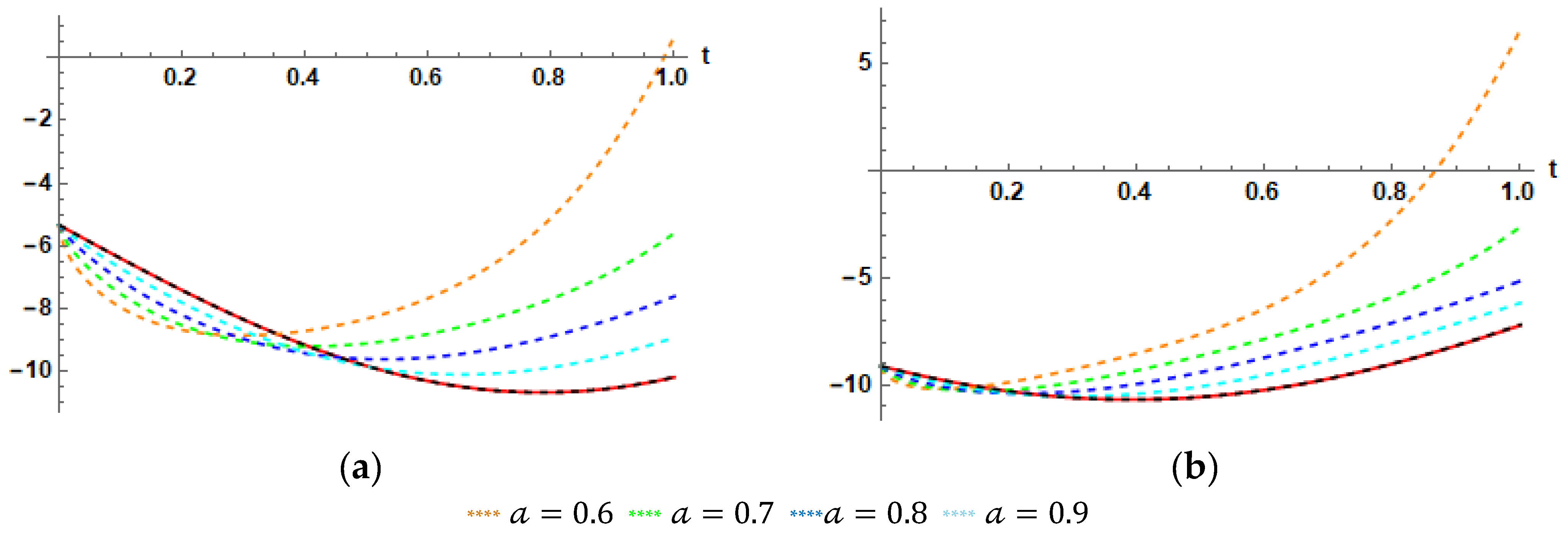
On the other hand, to show the effect of the fractional derivative to nonlinear time-fractional Rosenau–Hyman IVP (17), the graphs of the exact and 7-th approximate solutions for different values of $𝒶$ is established in Figure 3. Further, the geometric behavior of the exact and 7-th approximate solutions are plotted in 3D surface plots for $t\in \left[0,1\right]$, and $x\in \left[0,2\pi \right]$, at various values of values of $𝒶,$ as shown in Figure 4. This shows that from these figures the obtained approximate solution converges continuously to the standard-case $𝒶$ = 1 as $𝒶$ moves over $\left(0,1\right)$, and that the graphs of the behavior of the obtained 7-th approximate solution are consistent with each other, especially when considering the standard derivative.

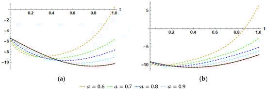
Figure 3. Profile the 7-th approximate solutions ${\mathcal{W}}_7\left(x,t\right),$ at various values of $𝒶$, for the nonlinear time-fractional Rosenau–Hyman IVP (17): (a) $x=\pi , c=4$; (b) $x=\frac{\pi }{2}, c=4$.

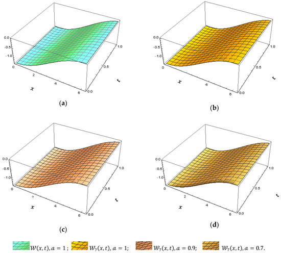
Figure 4. 3D Surface Plots of Exact solution $\mathcal{W}\left(x,t\right)$, and the 7-th approximate solution ${\mathcal{W}}_7\left(x,t\right)$, for IVP (17), with $t\in \left[0,1\right]$, and $x\in \left[0,2\pi \right]$, at various values of $𝒶$.

5. Conclusions

In this article, the approximate analytical solution is constructed and analyzed for nonlinear time-fractional Kolmogorov, and Rosenau–Hyman equations with suitable initial conditions utilizing the Laplace RPSM under time-Caputo differentiability. The present approach is a modification of the fractional RPSM via coupling it to the Laplace transform operator. The benefit of utilizing the Laplace RPSM is that it gives more accurate convergence McLaurin series and needs a small size of computation without involving the discretization, perturbation, or any other physical restrictive conditions. Two well-known physical applications are tested to validate the applicability and superiority of the proposed method. The obtained approximate solutions are discussed via graphics and numeric simulation. The obtained results are compared with other well-known existing methods in the literature. Therefore, the results confirm that the Laplace RPSM is a straightforward and convenient tool to deal with the range of various non-linear time fractional-PDEs that arise in engineering and science problems. In future studies, the Laplace RPSM can be extended to find exact and approximate solutions for systems of FPDEs. Consequently, the application of the Laplace RPSM can be extended to handle physical models and dynamical models.

References

- Mainardi, F.; Raberto, M.; Gorenflo, R.; Scalas, E. Fractional calculus and continuous-time finance II: The waiting-time distribution. Phys. A Stat. Mech. Its Appl. 2000, 287, 468–481. [Google Scholar] [CrossRef] [Green Version]
- He, J.H. Some applications of nonlinear fractional differential equations and their approximations. Bull. Sci. Technol. 1999, 15, 86–90. [Google Scholar]
- Caputo, M. Linear models of dissipation whose Q is almost frequency independent—II. Geophys. J. Int. 1967, 13, 529–539. [Google Scholar] [CrossRef]
- Oldham, K.B.; Spanier, J. The Fractional Calculus. In Integrations and Differentiations of Arbitrary Order; Descartes Press: Cambridge, MA, USA, 1974. [Google Scholar]
- Podlubny, I. Fractional Differential Equations; Academic Press: Cambridge, MA, USA, 1999. [Google Scholar]
- Alabedalhadi, M.; Al-Smadi, M.; Abu Arqub, O.; Baleanu, D.; Momani, S. Structure of optical soliton solution for nonlinear resonant space-time Schrödinger equation in conformable sense with full nonlinearity term. Physica Scripta. 2020, 95, 105215. [Google Scholar] [CrossRef]
- Al-Smadi, M.; Abu Arqub, O. Computational algorithm for solving fredholm time-fractional partial integrodifferential equations of Dirichlet functions type with error estimates. Appl. Math. Comput. 2019, 342, 280–294. [Google Scholar] [CrossRef]
- Al-Smadi, M.; Abu Arqub, O.; Hadid, S. An attractive analytical technique for coupled system of fractional partial differential equations in shallow water waves with conformable derivative. Commun. Theor. Phys. 2020, 72, 085001. [Google Scholar] [CrossRef]
- Jleli, M.; Kumar, S.; Kumar, R.; Samet, B. Analytical approach for time fractional wave equations in the sense of Yang-Abdel-Aty-Cattani via the homotopy perturbation transform method. Alex. Eng. J. 2020, 59, 2859–2863. [Google Scholar] [CrossRef]
- Hasan, S.; Al-Smadi, M.; Dutta, H.; Momani, S.; Hadid, S. Multi-step reproducing kernel algorithm for solving Caputo–Fabrizio fractional stiff models arising in electric circuits. Soft Comput. 2022, 26, 3713–3727. [Google Scholar] [CrossRef]
- Hasan, S.; El-Ajou, A.; Hadid, S.; Al-Smadi, M.; Momani, S. Atangana-Baleanu fractional framework of reproducing kernel technique in solving fractional population dynamics system. Chaos Solitons Fractals 2020, 133, 109624. [Google Scholar] [CrossRef]
- Al-Smadi, M.; Abu Arqub, O.; Momani, S. A computational method for two-point boundary value problems of fourth-order mixed integrodifferential equations. Math. Probl. Eng. 2013, 2013, 832074. [Google Scholar] [CrossRef]
- Al-Smadi, M.; Dutta, H.; Hasan, S.; Momani, S. On numerical approximation of Atangana-Baleanu-Caputo fractional integro-differential equations under uncertainty in Hilbert Space. Math. Model. Nat. Phenom. 2021, 16, 41. [Google Scholar] [CrossRef]
- Al-Smadi, M.; Abu Arqub, O.; Zeidan, D. Fuzzy fractional differential equations under the Mittag-Leffler kernel differential operator of the ABC approach: Theorems and applications. Chaos Solitons Fractals 2021, 146, 110891. [Google Scholar] [CrossRef]
- Al-Smadi, M.; Abu Arqub, O.; Gaith, M. Numerical simulation of telegraph and Cattaneo fractional-type models using adaptive reproducing kernel framework. Math. Methods Appl. Sci. 2021, 44, 8472–8489. [Google Scholar] [CrossRef]
- Wu, L.; Xie, L.d.; Zhang, J.f. Adomian decomposition method for nonlinear differential-difference equations. Commun. Nonlinear Sci. Numer. Simul. 2009, 14, 12–18. [Google Scholar] [CrossRef]
- Odibat, Z.; Momani, S. Application of variational iteration method to nonlinear differential equations of fractional order. Int. J. Nonlinear Sci. Numer. Simul. 2006, 7, 27–34. [Google Scholar] [CrossRef]
- Xu, H.; Liao, S.-J.; You, X.-C. Analysis of nonlinear fractional partial differential equations with the homotopy analysis method. Commun. Nonlinear Sci. Numer. Simul. 2009, 14, 1152–1156. [Google Scholar] [CrossRef]
- Hasan, S.; Al-Smadi, M.; El-Ajou, A.; Momani, S.; Hadid, S.; Al-Zhour, Z. Numerical approach in the Hilbert space to solve a fuzzy Atangana-Baleanu fractional hybrid system. Chaos Solitons Fractals 2021, 143, 110506. [Google Scholar] [CrossRef]
- Al-Smadi, M.; Freihat, A.; Khalil, H.; Momani, S.; Ali Khan, R. Numerical multistep approach for solving fractional partial differential equations. Int. J. Comput. Methods 2017, 14, 1750029. [Google Scholar] [CrossRef]
- Kumar, S. A new fractional modeling arising in engineering sciences and its analytical approximate solution. Alex. Eng. J. 2013, 52, 813–819. [Google Scholar] [CrossRef] [Green Version]
- Aljarrah, H.; Alaroud, M.; Ishak, A.; Darus, M. Adaptation of Residual-Error Series Algorithm to Handle Fractional System of Partial Differential Equations. Mathematics 2021, 9, 2868. [Google Scholar] [CrossRef]
- Saadeh, R.; Alaroud, M.; Al-Smadi, M.; Ahmad, R.R.; Din, U.K.S. Application of fractional residual power series algorithm to solve Newell–Whitehead–Segel equation of fractional order. Symmetry 2019, 11, 1431. [Google Scholar] [CrossRef] [Green Version]
- Freihet, A.; Hasan, S.; Alaroud, M.; Al-Smadi, M.; Ahmad, R.R.; Din, U.K.S. Toward computational algorithm for time-fractional Fokker–Planck models. Adv. Mech. Eng. 2019, 11, 1–11. [Google Scholar] [CrossRef]
- Al-Smadi, M.; Abu Arqub, O.; Hadid, S. Approximate solutions of nonlinear fractional Kundu-Eckhaus and coupled fractional massive Thirring equations emerging in quantum field theory using conformable residual power series method. Phys. Scr. 2020, 95, 105205. [Google Scholar] [CrossRef]
- Al-Smadi, M.; Abu Arqub, O.; Momani, S. Numerical computations of coupled fractional resonant Schrödinger equations arising in quantum mechanics under conformable fractional derivative sense. Phys. Scr. 2020, 95, 075218. [Google Scholar] [CrossRef]
- Alaroud, M.; Al-Smadi, M.; Ahmad, R.R.; Din, U.K.S. An analytical numerical method for solving fuzzy fractional Volterra integro-differential equations. Symmetry 2019, 11, 205. [Google Scholar] [CrossRef] [Green Version]
- Alaroud, M.; Al-Smadi, M.; Ahmad, R.R.; Din, U.K.S. Computational optimization of residual power series algorithm for certain classes of fuzzy fractional differential equations. Int. J. Differ. Equ. 2018, 2018, 8686502. [Google Scholar] [CrossRef]
- Alaroud, M.; Ahmad, R.R.; Din, U.K.S. An efficient analytical-numerical technique for handling model of fuzzy differential equations of fractional-order. Filomat 2019, 33, 617–632. [Google Scholar] [CrossRef] [Green Version]
- Bataineh, M.; Alaroud, M.; Al-Omari, S.; Agarwal, P. Series Representations for Uncertain Fractional IVPs in the Fuzzy Conformable Fractional Sense. Entropy 2019, 23, 1646. [Google Scholar] [CrossRef]
- El-Ajou, A. Adapting the Laplace transform to create solitary solutions for the nonlinear time-fractional dispersive PDEs via a new approach. Eur. Phys. J. Plu. 2021, 136, 229. [Google Scholar] [CrossRef]
- Alaroud, M. Application of Laplace residual power series method for approximate solutions of fractional IVP’s. Alex. Eng. J. 2022, 61, 1585–1595. [Google Scholar] [CrossRef]
- Alaroud, M.; Tahat, N.; Al-Omari, S.; Suthar, D.L.; Gulyaz-Ozyurt, S. An Attractive Approach Associated with Transform Functions for Solving Certain Fractional Swift-Hohenberg Equation. J. Funct. Spaces 2021, 2021, 3230272. [Google Scholar] [CrossRef]
- Yulita Molliq, R.; Noorani, M.S.M. Solving the fractional Rosenau-Hyman equation via variational iteration method and homotopy perturbation method. Int. J. Differ. Equ. 2012, 2012, 472030. [Google Scholar] [CrossRef] [Green Version]
- Korpinar, Z.; Inc, M.; Hınçal, E.; Baleanu, D. Residual power series algorithm for fractional cancer tumor models. Alex. Eng. J. 2020, 59, 1405–1412. [Google Scholar] [CrossRef]
- Nikan, O.; Avazzadeh, Z. Numerical simulation of fractional evolution model arising in viscoelastic mechanics. Appl. Num. Math. 2021, 169, 303–320. [Google Scholar] [CrossRef]
- Ali, A.; Abbas, M.; Akram, T. New group iterative schemes for solving the two-dimensional anomalous fractional sub-diffusion equation. J. Math. Comp. Sci. 2021, 22, 119–127. [Google Scholar] [CrossRef]
- Almatroud, A.; Ababneh, O.; Al-sawalha, M.M. Modify adaptive combined synchronization of fractional order chaotic systems with fully unknown parameters. J. Math. Comp. Sci. 2020, 21, 99–112. [Google Scholar] [CrossRef]
- Akram, T.; Abbas, M.; Ali, A. A numerical study on time fractional Fisher equation using an extended cubic B-spline approximation. J. Math. Comp. Sci. 2021, 22, 85–96. [Google Scholar] [CrossRef]
- Qu, H.; Rahman, M.; Ahmad, S.; Riaz, M.B.; Ibrahim, M.; Saeed, T. Investigation of fractional order bacteria dependent disease with the effects of different contact rates. Chaos Sol. Fract. 2022, 159, 112169. [Google Scholar] [CrossRef]
- El-Deeb, A.A.; Baleanu, D. Some new dynamic Gronwall–Bellman–Pachpatte type inequalities with delay on time scales and certain applications. J. Inequal. Appl. 2022, 2022, 45. [Google Scholar] [CrossRef]
- Kumar, P.; Baleanu, D.; Erturk, V.S.; Inc, M.; Govindaraj, V. A delayed plant disease model with Caputo fractional derivatives. Adv. Cont. Discr. Mod. 2022, 2022, 11. [Google Scholar] [CrossRef]
- Wang, G.; Wazwaz, A. On the modified Gardner type equation and its time fractional form. Chaos Solit. Fract. 2022, 155, 111694. [Google Scholar] [CrossRef]
- Wang, G. A new (3 + 1)-dimensional Schrödinger equation: Derivation, soliton solutions and conservation laws. Nonlin. Dyn. 2021, 104, 1595–1602. [Google Scholar] [CrossRef]
- Wang, G. Symmetry Analysis, Analytical Solutions And Conservation Laws Of A Generalized Kdv–Burgers–Kuramoto Equation And Its Fractional Version. Fractals 2021, 29, 2150101. [Google Scholar] [CrossRef]
- Wang, G. A novel (3 + 1)-dimensional sine-Gorden and a sinh-Gorden equation: Derivation, symmetries and conservation laws. Appl. Math. Lett. 2021, 113, 106768. [Google Scholar] [CrossRef]
- Wang, G. A (2 + 1)-dimensional sine-Gordon and sinh-Gordon equations with symmetries and kink wave solutions. Nucl. Phys. B 2020, 953, 114956. [Google Scholar] [CrossRef]
Publisher’s Note: MDPI stays neutral with regard to jurisdictional claims in published maps and institutional affiliations. |
© 2022 by the authors. Licensee MDPI, Basel, Switzerland. This article is an open access article distributed under the terms and conditions of the Creative Commons Attribution (CC BY) license (https://creativecommons.org/licenses/by/4.0/).