Modeling of Cerebral Blood Flow Autoregulation Using Mathematical Control Theory

Abstract

A mathematical model of cerebral blood flow in the form of a dynamical system is studied. The cerebral blood flow autoregulation modeling problem is treated as a nonlinear control problem and the potential and applicability of the nonlinear control theory techniques are analyzed in this respect. It is shown that the cerebral hemodynamics model in question is differentially flat. Then, the integrator backstepping approach combined with barrier Lyapunov functions is applied to construct the control laws that recover the cerebral autoregulation performance of a healthy human. Simulation results confirm the good performance and flexibility of the suggested cerebral blood flow autoregulation design. The conducted research should enrich our understanding of the mathematics behind the cerebral blood flow autoregulation mechanisms and medical treatments to compensate for impaired cerebral autoregulation, e.g., in preterm infants.

1. Introduction

Understanding the mathematics behind the cerebral autoregulation process is of primary importance in the mathematical modeling of cerebral blood circulation and regulation. Impaired cerebral blood flow autoregulation is one of the crucial factors that can cause cerebral hemorrhage in preterm infants. An impaired cerebral autoregulation mechanism is unable to maintain constant cerebral blood flow despite the changes in systemic arterial pressure. As a result, an increase in cerebral blood flow caused by an acute systemic arterial pressure increase can lead to bleeding in the germinal matrix of a preterm newborn [1], which is a specific region in the immature brain between the thalamus and caudate nucleus, with high vascularity and a fragile capillary network [2]. Among a variety of cerebral blood flow models (see, e.g., [3,4,5,6,7,8,9,10,11]), one can highlight lumped parameter models based on the analogy to electric circuits [4,5,6,7,8,9,10]. In [9,10], the influence of the germinal matrix on blood flow is taken into account by modeling the capillary level as two parallel connected lumped objects describing the germinal matrix and the remaining part of the brain. In [4], a cerebral blood flow model is presented in the form of nonlinear ordinary differential equations, which can be seen as a starting point to the automatic control theory oriented cerebral autoregulation modeling, because of its simplicity and, at the same time, ability to reproduce various clinical results [4].

The first steps towards considering the cerebral blood flow autoregulation modeling problem as a feedback control problem were undertaken in [7,8]. In [7], maintenance of the cerebral autoregulatory function was studied as an optimal conflict control problem. In [8], a mathematical model of cerebral autoregulation was proposed in the form of a heuristic feedback controller, verified using the techniques of the viability theory [12].

In the current work, we continue to develop the automatic control theory-based autoregulation considerations in a systemic way. Based on the cerebral blood flow dynamical model of [4], the nonlinear control theory tools are applied to construct the feedback control laws that describe the mathematics behind the cerebral autoregulation mechanisms. The main results of this paper originate from the suggested idea to interpret the cerebral blood flow autoregulation modeling challenge as an automatic control problem. This is the first time, at least to our knowledge, that the cerebral blood flow model introduced in [4] is studied as a dynamical system with control input and its controllability properties are analyzed. Because of the model’s intrinsic nonlinearity, such a well-known and effective nonlinear control tool as integrator backstepping combined with barrier Lyapunov functions is used to construct the control laws that recover the cerebral autoregulation performance of healthy humans.

The remaining part of the paper is organized as follows. In Section 2, the cerebral hemodynamics model equations presented in [4] are revisited and written in the form of a nonlinear dynamical system with control input. The cerebral blood flow autoregulation modeling problem is formulated as a nonlinear output tracking control problem. In Section 3, we show the differential flatness property of the cerebral hemodynamics in question, which is used further in Section 4 to construct the state feedback control laws that model the cerebral autoregulation performance. Numerical simulation results of the suggested cerebral blood flow autoregulation scheme are given in Section 4. Finally, Section 5 concludes with some remarks.

2. Problem Formalization

In this paper, we consider the cerebral hemodynamics model introduced in [4]. For convenience’s sake, let us first summarize the model equations. The model accounts for the hemodynamics of the arterial–arteriolar cerebrovascular bed and large cerebral veins, cerebrospinal fluid circulation and intracranial pressure dynamics; see Figure 1. The arterial–arteriolar cerebrovascular bed is modeled as a windkessel and is described by means of the hydraulic compliance (storage capacity) $C_a$ and the hydraulic resistance $R_a$ variables [4]. The arterial–arteriolar blood volume $V_a$ is calculated as below

$$V_a=C_a(P_a-P_{ic}),$$

(1)

where $P_a$ and $P_{ic}$ stand for the systemic arterial and intracranial pressure variables, respectively. The difference $P_a-P_{ic}$ represents transmural pressure in the arterioles. The rate q of blood flow through the arterial–arteriolar cerebrovascular bed that enters the skull is written as

$$q=\frac{P_a-P_c}{R_a},$$

(2)

where $P_c$ denotes the capillary pressure variable, and the difference $P_a-P_c$ is the perfusion pressure of the arterioles. Here, by the Hagen–Poiseuille law, the arterial–arteriolar resistance $R_a$ is inversely proportional to the second power of the blood volume $V_a$ with a coefficient $k_R^{\prime }$ [4], i.e.,

$$R_a=\frac{k_R^{\prime }}{V_a^2}.$$

(3)

Figure 1. The cerebral hemodynamics model components and quantities.

For the large intracranial veins, autoregulatory mechanisms and venous elasticity are neglected. The transmural pressure in the cerebral veins and the venous blood volume are supposed to remain constant. Then, the rate $q_v$ of the blood flow through the venous cerebrovascular bed is described using a hydraulic resistance $R_{pv}$ as

$$q_v=\frac{P_c-P_{ic}}{R_{pv}},$$

(4)

with the venous hydraulic compliance being ignored and $R_{pv}$ treated as a constant [4]. Here, in (4), the difference $P_c-P_{ic}$ represents the perfusion pressure of the cerebral veins. Similarly, cerebrospinal fluid production at the cerebral capillaries and reabsorption at the dural sinuses are modeled as static processes. The cerebrospinal fluid production and reabsorption rates $q_f$ and $q_o$ are characterized by constant hydraulic resistances $R_f$ and $R_o$, respectively, as below

$$q_f=\frac{P_c-P_{ic}}{R_f},q_o=\frac{P_{ic}-P_{vs}}{R_o},$$

(5)

where $P_{vs}$ is the venous sinus pressure, which is taken as a constant [4]. The quantities q, $q_v$ and $q_f$ given by the Formulae (2), (4) and (5) are linked through the algebraic equation

$$q=q_v+q_f.$$

(6)

The intracranial pressure $P_{ic}$ dynamics by Monro–Kellie doctrine are written as follows [4]:

$$C_{ic}{\dot{P}}_{ic}={\dot{V}}_a+q_f-q_o+I_i,$$

(7)

where $C_{ic}$ is the intracranial compliance (craniospinal storage capacity), and $I_i$ stands for the constant rate of possible mock cerebrospinal fluid injection in surgery. In (7), the intracranial storage capacity $C_{ic}$ is inversely proportional to the intracranial pressure $P_{ic}$ with a craniospinal compartment elastance coefficient $k_E$, i.e.,

$$C_{ic}=\frac{1}{k_E{P}_{ic}}.$$

(8)

Moreover, one should note that the following condition $P_a>P_c>P_{ic}>P_{vs}$ on the pressure values is required to hold for all the above considerations to be valid [4].

Finally, within the cerebral hemodynamics model in question, cerebral blood flow autoregulation is supposed to function only at the level of arterioles and is described in terms of the arterial–arteriolar compliance $C_a$. Vasodilation or vasoconstriction of the arterioles is modeled through positive or negative values of the compliance rate ${\dot{C}}_a$, respectively. In [4], the following heuristic cerebral autoregulation model is suggested:

$${\dot{C}}_a=\frac{1}{\tau }\left(-C_a+\sigma \left(\frac{q-q_n}{q_n}\right)\right),$$

(9)

where $\sigma (·)$ is a sigmoidal function with saturation, $\tau$ is a time constant, and $q_n$ denotes a basal value of the arterial–arteriolar blood flow rate q required for tissue metabolism.

Notice that the cerebral autoregulation model (9) is intuitively clear but the authors do not provide any mathematical proof or strict mathematical considerations of its validity in [4]. In this paper, as is done in [7], the arterial–arteriolar compliance rate ${\dot{C}}_a$ is considered as a control input. Then, the control purpose is to force the nonzero values of the difference $q\left(t\right)-q_n$ to zero using nonlinear control theory tools and, thus, provide rigorous mathematical insights into the cerebral blood flow autoregulation mechanism of a healthy human.

In the current work, we adopt the arterial–arteriolar blood volume $V_a$ and the intracranial pressure $P_{ic}$ as system state variables, instead of considering the $C_a$ and $P_{ic}$ dynamics, as is done in [4]. This choice of the state variables is more suitable for a thorough analysis of the cerebral hemodynamics in question and control design since $V_a$ is a crucial quantity defining the behavior of the overall system. In view of (1), the blood volume $V_a$ dynamics are governed by the formula

$${\dot{V}}_a={\dot{C}}_a(P_a-P_{ic})+C_a({\dot{P}}_a-{\dot{P}}_{ic})$$

(10)

and are determined by the cerebral autoregulation mechanism ${\dot{C}}_a$, the intracranial pressure dynamics ${\dot{P}}_{ic}$ and the systemic arterial pressure alterations rate ${\dot{P}}_a$.

After rearranging the terms in the differential-algebraic Equations (7) and (10) and taking into account the relations (5) and (8), one can avoid algebraic loops and obtain the following dynamical system:

$$\begin{array}{cc}\hfill & {\dot{V}}_a=\frac{1}{1+k_E{P}_{ic}{C}_a}\left(-k_E{P}_{ic}{C}_a\left(\frac{P_c-P_{ic}}{R_f}-\frac{P_{ic}-P_{vs}}{R_0}+I_i\right)+(P_a-P_{ic}){\dot{C}}_a+C_a{\dot{P}}_a\right),\hfill \\ \hfill & {\dot{P}}_{ic}=\frac{k_E{P}_{ic}}{1+k_E{P}_{ic}{C}_a}\left(\frac{P_c-P_{ic}}{R_f}-\frac{P_{ic}-P_{vs}}{R_0}+I_i+(P_a-P_{ic}){\dot{C}}_a+C_a{\dot{P}}_a\right)\hfill \end{array}$$

(11)

which describes time behavior of the cerebral blood volume $V_a$ and the intracranial pressure $P_{ic}$. Using the Formulae (1)–(6), the capillary pressure $P_c$ and the arterial–arteriolar compliance $C_a$ quantities in the right-hand side of the system (11) can be represented as functions of the system state variables $V_a$ and $P_{ic}$ in the following way:

$$P_c=P_c(V_a,P_{ic})=\frac{R_f{R}_{pv}{P}_a{V}_a^2+k_R^{\prime }(R_{pv}+R_f)P_{ic}}{k_R^{\prime }(R_{pv}+R_f)+R_f{R}_{pv}{V}_a^2},$$

(12)

$$C_a=C_a(V_a,P_{ic})=\frac{P_a-P_{ic}}{V_a}.$$

Notice that the functions in the right-hand side of the system (11) depend on the systemic arterial pressure $P_a$ time behavior. In this paper, we suppose that the arterial blood pressure dynamics are in a steady state, i.e., ${\dot{P}}_a\equiv 0$, and the arterial pressure $P_a$ has a constant value, which is possibly different from the basal one. Then, the choice of the arterial–arteriolar compliance rate ${\dot{C}}_a$ as a control input u results in the cerebral hemodynamics model

$$\begin{array}{cc}\hfill & {\dot{V}}_a=\frac{1}{1+k_E{P}_{ic}{C}_a}\left(-k_E{P}_{ic}{C}_a\left(\frac{P_c-P_{ic}}{R_f}-\frac{P_{ic}-P_{vs}}{R_0}+I_i\right)+(P_a-P_{ic})u\right),\hfill \\ \hfill & {\dot{P}}_{ic}=\frac{k_E{P}_{ic}}{1+k_E{P}_{ic}{C}_a}\left(\frac{P_c-P_{ic}}{R_f}-\frac{P_{ic}-P_{vs}}{R_0}+I_i+(P_a-P_{ic})u\right),\hfill \end{array}$$

(13)

with the arterial-,arteriolar blood flow rate q being considered as a system output function and in view of (2), (3) and (12), written as

$$q=q(V_a,P_{ic})=\frac{(R_{pv}+R_f)(P_a-P_{ic})V_a^2}{k_R^{\prime }(R_{pv}+R_f)+R_f{R}_{pv}{V}_a^2}.$$

(14)

Thus, in summary, the cerebrovascular autoregulation modeling problem in question can be formulated as a constrained (e.g., asymptotic) output regulation control problem for the nonlinear dynamical system (13), i.e., we find a feedback control law $u=u(V_a,P_{ic})$ such that

$$|q(V_a\left(t\right),P_{ic}\left(t\right))-q_n|\to 0\mathrm{as}t\to +\infty$$

(15)

for all reasonable initial values $V_a\left(0\right)={V_a}_0$, $P_{ic}\left(0\right)={P_{ic}}_0$ of the system state variables. In addition, for a proper range of the systemic arterial pressure values $P_a\in [P_{amin},P_{amax}]$, the quantities $V_a\left(t\right)$ and $P_{ic}\left(t\right)$ are required to remain positive during transients and within reasonable bounds

$$V_a\left(t\right)\in [V_{amin},V_{amax}],P_{ic}\left(t\right)\in [P_{icmin},P_{icmax}],t\ge 0.$$

(16)

3. Differential Flatness of Cerebral Hemodynamics

First, let us check the controllability properties of the nonlinear dynamical system (13) by showing that it is differentially flat [13]. Recall that a dynamical system of the form (13) is differentially flat if and only if there exists a scalar function $z_1$ of the system state variables $V_a$, $P_{ic}$ and, in a general case, of the control input u with its time derivatives $\dot{u}$, $\ddot{u}$, ⋯, $u^{\left(\alpha \right)}$ for some finite natural number $\alpha$ such that $V_a$, $P_{ic}$ and u can be represented as functions of $z_1$ and its time derivatives of up to some finite order [13]. Then, it is well known that differentially flat systems possess good controllability properties (see, e.g., [13,14]). To find such a function $z_1$, called the flat output, one can exploit the linearity of the functions on the right-hand side of the system (13) with respect to the control variable u. The coefficients of u in (13) form the vector field

$$B(V_a,P_{ic})=\frac{P_a-P_{ic}}{(1+k_E{P}_{ic}{C}_a)}\left(\begin{array}{c}1\\ k_E{P}_{ic}\end{array}\right).$$

(17)

As a flat output candidate for the system (13), one can take a first integral of the vector field (17) (see, e.g., [15]). To find the first integrals of $B(V_a,P_{ic})$ given by (17), consider an auxiliary system of ordinary differential equations written in the symmetric form

$$\frac{d{V}_a}{1}=\frac{d{P}_{ic}}{k_E{P}_{ic}}=dt.$$

(18)

Integration of (18) results in the following function:

$$z_1={\phi }_1(V_a,P_{ic})=k_E{V}_a-ln{P}_{ic}$$

(19)

which has constant values on solutions of the auxiliary system (18), with its Lie derivative $L_B{\phi }_1$ [15] along the vector field $B(V_a,P_{ic})$ being identically zero. Then, the first- and second-order time derivatives of (19) along solutions of the dynamical system (13) can be written, respectively, as

$${\dot{z}}_1=k_E{\dot{V}}_a-\frac{{\dot{P}}_{ic}}{P_{ic}}={\phi }_2(V_a,P_{ic})=\frac{-k_E{R}_{pv}}{R_{pv}+R_f}q+\frac{k_E}{R_o}{P}_{ic}-k_E\left(\frac{P_{vs}}{R_o}+I_i\right),$$

(20)

$$\begin{array}{cc}\hfill {\ddot{z}}_1=& \frac{-k_E{R}_{pv}}{R_{pv}+R_f}\dot{q}+\frac{k_E}{R_0}{\dot{P}}_{ic}=\frac{-k_E{R}_{pv}}{R_{pv}+R_f}\left(\frac{\partial q}{\partial V_a}{\dot{V}}_a+\frac{\partial q}{\partial P_{ic}}{\dot{P}}_{ic}\right)+\frac{k_E}{R_0}{\dot{P}}_{ic}\hfill \\ \hfill =& f(V_a,P_{ic})+g(V_a,P_{ic})u,\hfill \end{array}$$

(21)

where $f(·)$ and $g(·)$ are corresponding functions of their arguments.

Let $z_2={\dot{z}}_1$, $z={(z_1,z_2)}^{\mathrm{T}}$ and $\Phi (V_a,P_{ic})={({\phi }_1(V_a,P_{ic}),{\phi }_2(V_a,P_{ic}))}^{\mathrm{T}}$. One can show that the Jacobian matrix of the mapping $z=\Phi (V_a,P_{ic})$ defined by the relations (19) and (20) is nonsingular at a point $V_a={V_a}_0$, $P_{ic}={P_{ic}}_0$ if and only if the following condition holds:

$$q({V_a}_0,{P_{ic}}_0)\ne \frac{k_E(R_{pv}{R}_o+R_f{R}_{pv}){P_{ic}}_0{V_a}_0^3+k_R^{\prime }{k}_E(R_{pv}+R_f){P_{ic}}_0{V_a}_0}{2k_R^{\prime }{R}_{pv}{R}_o}.$$

(22)

Hence, the map $z=\Phi (V_a,P_{ic})$ is a diffeomorphism defined for all values $V_a={V_a}_0$, $P_{ic}={P_{ic}}_0$ such that the inequality (22) is satisfied. The relationships (19) and (20) qualify as a change of coordinates in the state space of the system (13), with its inversion being written as ${(V_a,P_{ic})}^{\mathrm{T}}={\Phi }^{-1}\left(z\right)$. Thus, the system state variables $V_a$, $P_{ic}$ are expressed as functions of the flat output $z_1$ given by (19) and its time derivative ${\dot{z}}_1$ defined as (20). Finally, from (21), we deduce that the control variable u can be represented for the nonzero values of $g(V_a,P_{ic})\ne 0$ as below

$$u=u(z_1,{\dot{z}}_1,{\ddot{z}}_1)=\frac{1}{\tilde{g}\left(z\right)}({\ddot{z}}_1-\tilde{f}\left(z\right)),$$

(23)

where

$$\tilde{g}\left(z\right)={\left[g(V_a,P_{ic})\right]}_{{(V_a,P_{ic})}^{\mathrm{T}}={\Phi }^{-1}\left(z\right)},\tilde{f}\left(z\right)={\left[f(V_a,P_{ic})\right]}_{{(V_a,P_{ic})}^{\mathrm{T}}={\Phi }^{-1}\left(z\right)}.$$

(24)

Note that one can check that the inequality $g(V_a,P_{ic})\ne 0$ at a point $V_a={V_a}_0$, $P_{ic}={P_{ic}}_0$ is equivalent to the condition (22). This fact is an outcome of a more general theory of nonlinear dynamical systems presented in [15]. As a consequence of the above considerations, we conclude that the system (13) is differentially flat.

4. Nonlinear Output Regulation Control Design

To guarantee the cerebral blood flow regulation (15), one can first try to find the constant reference values $V_a={V_a}_r=\mathrm{const}$ and $P_{ic}={P_{ic}}_r=\mathrm{const}$ such that the condition $q({V_a}_r,{P_{ic}}_r)=q_n$ holds. Then, a reasonable control strategy would be to force the differences $V_a\left(t\right)-{V_a}_r$ and $P_{ic}\left(t\right)-{P_{ic}}_r$ to zero as $t\to +\infty$ in a controllable way to meet the constraints (16) by the choice of a state feedback $u=u(V_a,P_{ic})$.

In this paper, the reference value ${P_{ic}}_r$ of the intracranial pressure variable $P_{ic}$ let us select to nullify the $z_1$ rate given by (20) under the basal value $q=q_n$ of the arterial-arteriolar blood flow rate, i.e.,

$${P_{ic}}_r=\frac{R_o{R}_{pv}{q}_n}{R_{pv}+R_f}+P_{vs}+R_o{I}_i.$$

(25)

One can easily check that the right-hand side of the expression (25) under the basal values of model parameters given in [4] and revised for convenience’s sake in Table 1 coincides with a basal value of the intracranial pressure $P_{ic}$ in a healthy human [16]. Note that, in case some of the model parameter values in (25) differ from the basal ones of a healthy human, still, one could use, for instance, the constant rate of mock cerebrospinal fluid injection $I_i$ to obtain a reference value ${P_{ic}}_r$ of the intracranial pressure that stays within medically reasonable bounds [16].

Table 1. Model parameters in basal conditions.

Model Parameter	Basal Value
$q_n$	12.5 $\mathrm{mL}·{\mathrm{s}}^{-1}$
$R_{pv}$	1.24 $\mathrm{mmHg}·\mathrm{s}·{\mathrm{mL}}^{-1}$
$R_f$	$2.38\times {10}^3$$\mathrm{mmHg}·\mathrm{s}·{\mathrm{mL}}^{-1}$
$R_o$	526.3 $\mathrm{mmHg}·\mathrm{s}·{\mathrm{mL}}^{-1}$
$P_{vs}$	6.0 mmHg
$k_E$	0.11 ${\mathrm{mL}}^{-1}$
$k_R^{\prime }$	$0.11\times {10}^4$$\mathrm{mmHg}·\mathrm{s}·\mathrm{mL}$
$I_i$	0 $\mathrm{mL}·{\mathrm{s}}^{-1}$

Then, from the relations (14) and $q({V_a}_r,{P_{ic}}_r)=q_n$, it is deduced that

$${V_a}_r=\sqrt{\frac{k_R^{\prime }(R_{pv}+R_f)q_n}{(R_{pv}+R_f)(P_a-{P_{ic}}_r)-R_{pv}{R}_f{q}_n}}.$$

(26)

Note that, for the reference blood volume value (26) to be correctly defined, the following conditions on the model parameters and the intracranial pressure reference value have to be satisfied:

$$P_a>\frac{R_{pv}{R}_f{q}_n}{R_{pv}+R_f}+{P_{ic}}_r,{V_a}_r\in [V_{amin},V_{amax}].$$

(27)

It is worthwhile to indicate that the validity of the relationships (27) is inherently related to the model parameters’ consistency and can be easily verified for the parameter values given in Table 1 within the systemic arterial pressure $P_a$ autoregulatory lower and upper limits $P_{amin}=60$ mmHg and $P_{amax}=160$ mmHg, respectively [4].

In what follows, we exploit the differential flatness property of the cerebral hemodynamics model (13) conceived in the above section. In the new coordinates $z={(z_1,z_2)}^{\mathrm{T}}$ defined by the Formulae (19) and (20), the dynamical system (13) takes the form

$$\begin{array}{cc}\hfill & {\dot{z}}_1=z_2,\hfill \\ \hfill & {\dot{z}}_2=\tilde{f}(z_1,z_2)+\tilde{g}(z_1,z_2)u,\hfill \end{array}$$

(28)

with the functions on its right-hand side being introduced in (24). Further, in view of (19) for the $z_1$ variable, we take the reference value ${z_1}_r=k_E{V_a}_r-ln{P_{ic}}_r$, where ${P_{ic}}_r$ and ${V_a}_r$ are given by (25) and (26), respectively. Moreover, by combining the relations (20) and (25), one obtains ${z_2}_r=0$ as the reference value of the $z_2$ variable.

To achieve the regulation $z_1\left(t\right)-{z_1}_r\to 0$ and $z_2\left(t\right)\to 0$ as $t\to +\infty$, a straightforward control selection would be the state feedback linearization-based design

$$u=\frac{1}{\tilde{g}(z_1,z_2)}\left(-\tilde{f}(z_1,z_2)-c_1(z_1-{z_1}_r)-c_2{z}_2\right)$$

(29)

which results in the following regulation error dynamics:

$$\begin{array}{cc}\hfill \dot{\overbrace{z_1-{z_1}_r}}& =z_2,\hfill \\ \hfill {\dot{z}}_2& =-c_1(z_1-{z_1}_r)-c_2{z}_2.\hfill \end{array}$$

(30)

Then, for any positive gain coefficients $c_1>0$ and $c_2>0$, the equilibrium point $z_1={z_1}_r$, $z_2=0$ of the system (30) is (globally) asymptotically stable.

Notice that the control law (29) and, hence, the resultant closed-loop dynamics (30) are defined whenever the control coefficient $\tilde{g}(z_1,z_2)$ in (28) is not zero. It can be shown that the inequality $\tilde{g}(z_1,z_2)\ne 0$ holds for the reference values $V_a={V_a}_r$, $P_{ic}={P_{ic}}_r$ of the arterial–arteriolar blood volume and intracranial pressure variables defined as (25) and (26), respectively, under the autoregulatory range of the systemic arterial pressure values $P_a\in [60,160]$ mmHg and model parameter basal values given in Table 1. Hence, due to the continuity property of the function $\tilde{g}(·)$, the condition $\tilde{g}(z_1,z_2)\ne 0$ is satisfied at least in some neighborhood of the point $z_1={z_1}_r$, $z_2=0$ of the system (28) state space.

It is well known that the control law (29) cannot explicitly guarantee that the nontrivial trajectories $z_1=z_1\left(t\right)\not\equiv {z_1}_r$, $z_2=z_2\left(t\right)\not\equiv 0$ of the closed-loop dynamics (30) (and, hence, the variables $V_a\left(t\right)$ and $P_{ic}\left(t\right)$ during the cerebral autoregulation transients) remain bounded within the prescribed bounds for all $t\ge 0$ or do not approach and become stuck in the set $\tilde{g}(z_1,z_2)=0$ ($g(V_a,P_{ic})=0$).

To avoid the control singularity, i.e., obtaining $g(V_a\left(t\right),P_{ic}\left(t\right))=0$ at some $t=t_{*}$, let us redesign the control law (29) to provide the conditions

$$|V_a\left(t\right)-{V_a}_r|\le L_1,|P_{ic}\left(t\right)-{P_{ic}}_r|\le L_2,t\ge 0$$

(31)

with proper positive bounds $L_1$, $L_2$ consistent with the constraints (16). Notice that, since $g({V_a}_r,{P_{ic}}_r)\ne 0$, which, by virtue of the relations (24), is equivalent to the inequality $\tilde{g}({z_1}_r,0)\ne 0$, there always exist positive constants $L_1$, $L_2$ such that, from (31), it can be deduced that $g(V_a\left(t\right),P_{ic}\left(t\right))\ne 0$ for all $t\ge 0$. Then, since the change of coordinates $z=\Phi (V_a,P_{ic})$ given by (19) and (20) defines a diffeomorphism whenever $g(V_a,P_{ic})\ne 0$, the inequalities (31) can be rewritten in the variables $z_1$, $z_2$ as

$$|z_1\left(t\right)-{z_1}_r|\le M_1,\left|z_2\left(t\right)\right|\le M_2,t\ge 0$$

(32)

with some relevant bounds $M_1=M_1(L_1,L_2)$ and $M_2=M_2(L_1,L_2)$.

To provide the regulation $z_1\left(t\right)-{z_1}_r\to 0$, $z_2\left(t\right)\to 0$ as $t\to +\infty$ and satisfy the conditions (32) on the transients simultaneously, we suggest to redesign the control law (29) by using the integrator backstepping approach [17] based on barrier Lyapunov functions; see, e.g., [18].

To this end, consider first a (barrier) function

$$V_1\left({\xi }_1\right)=\frac{1}{2}{k}_{1}ln\left(\frac{N_1^2}{N_1^2-{\xi }_1^2}\right),$$

where ${\xi }_1=z_1-{z_1}_r$, $N_1=M_1$, $k_1$ is a positive design constant. Introduce the error variable ${\xi }_2=z_2-{\alpha }_1\left({\xi }_1\right)$. Here, ${\alpha }_1(·)$ is a continuously differentiable function to be defined later, which accounts for the desired reference behavior of the $z_2$ variable.

The time derivative of $V_1\left({\xi }_1\right)$ along solutions of the system (28) is written as

$${\dot{V}}_1\left({\xi }_1\right)=\frac{k_1{\xi }_1{\dot{\xi }}_1}{N_1^2-{\xi }_1^2}=\frac{k_1{\xi }_1{z}_2}{N_1^2-{\xi }_1^2}=\frac{k_1{\xi }_1{\alpha }_1\left({\xi }_1\right)}{N_1^2-{\xi }_1^2}+\frac{k_1{\xi }_1{\xi }_2}{N_1^2-{\xi }_1^2}.$$

The choice ${\alpha }_1\left({\xi }_1\right)=-{\kappa }_1{\xi }_1$, where ${\kappa }_1>0$ is a positive gain coefficient, results in

$${\dot{V}}_1\left({\xi }_1\right)=-\frac{k_1{\kappa }_1{\xi }_1^2}{N_1^2-{\xi }_1^2}+\frac{k_1{\xi }_1{\xi }_2}{N_1^2-{\xi }_1^2}.$$

Hence, ${\dot{V}}_1\left({\xi }_1\right)$ is negative definite if ${\xi }_2\left(t\right)\equiv 0$.

Then, as a Lyapunov function candidate for the whole system, employ the barrier function

$$V_2({\xi }_1,{\xi }_2)=V_1\left({\xi }_1\right)+\frac{1}{2}{k}_{2}ln\left(\frac{N_2^2}{N_2^2-{\xi }_2^2}\right),$$

where $N_2=M_2-{\kappa }_1{M}_1$, $k_2>0$ is some positive design constant. Let the values ${\kappa }_1>0$ and $M_1>0$, $M_2>0$ be such that $N_2>0$. Note that the function $V_2({\xi }_1,{\xi }_2)$ is positive definite in the domain $\{({\xi }_1,{\xi }_2)\in {\mathbb{R}}^2:|{\xi }_1|<N_1,|{\xi }_2|<N_2\}$ and grows unbounded $V_2({\xi }_1,{\xi }_2)\to +\infty$ as ${\xi }_1\to N_1-0$ or/and ${\xi }_2\to N_2-0$.

The time derivative of $V_2({\xi }_1,{\xi }_2)$ along solutions of the system (28) is calculated as below

$$\begin{array}{cc}\hfill {\dot{V}}_2({\xi }_1,{\xi }_2)& =-\frac{k_1{\kappa }_1{\xi }_1^2}{N_1^2-{\xi }_1^2}+\frac{k_1{\xi }_1{\xi }_2}{N_1^2-{\xi }_1^2}+\frac{k_2{\xi }_2{\dot{\xi }}_2}{N_2^2-{\xi }_2^2}\hfill \\ \hfill & =-\frac{k_1{\kappa }_1{\xi }_1^2}{N_1^2-{\xi }_1^2}+\frac{k_1{\xi }_1{\xi }_2}{N_1^2-{\xi }_1^2}+\frac{k_2{\xi }_2\left(\tilde{f}(z_1,z_2)+\tilde{g}(z_1,z_2)u+{\kappa }_1{z}_2\right)}{N_2^2-{\xi }_2^2}.\hfill \end{array}$$

The control selection

$$u=\frac{1}{\tilde{g}(z_1,z_2)}\left(-\tilde{f}(z_1,z_2)-{\kappa }_1{z}_2-{\kappa }_2{\xi }_2-{\xi }_2(N_2^2-{\xi }_2^2)\right),$$

(33)

where ${\kappa }_2>0$ is a positive gain coefficient, yields

$${\dot{V}}_2({\xi }_1,{\xi }_2)=-\frac{k_1{\kappa }_1{\xi }_1^2}{N_1^2-{\xi }_1^2}+\frac{k_1{\xi }_1{\xi }_2}{N_1^2-{\xi }_1^2}-\frac{k_2{\kappa }_2{\xi }_2^2}{N_2^2-{\xi }_2^2}-k_2{\xi }_2^2.$$

By completing the squares, one obtains

$$\begin{array}{cc}\hfill {\dot{V}}_2({\xi }_1,{\xi }_2)& =-\frac{k_1{\kappa }_1{\xi }_1^2}{2(N_1^2-{\xi }_1^2)}-\left(\frac{k_1{\kappa }_1{\xi }_1^2}{2(N_1^2-{\xi }_1^2)}-\frac{k_1{\xi }_1{\xi }_2}{N_1^2-{\xi }_1^2}+\frac{k_1{\xi }_2^2}{2{\kappa }_1(N_1^2-{\xi }_1^2)}\right)-\frac{k_2{\kappa }_2{\xi }_2^2}{N_2^2-{\xi }_2^2}\hfill \\ \hfill & -{\xi }_2^2\left(k_2-\frac{k_1}{2{\kappa }_1(N_1^2-{\xi }_1^2)}\right)=-\frac{k_1{\kappa }_1{\xi }_1^2}{2(N_1^2-{\xi }_1^2)}-\frac{k_2{\kappa }_2{\xi }_2^2}{N_2^2-{\xi }_2^2}\hfill \\ \hfill & -{\left({\xi }_1\sqrt{\frac{k_1{\kappa }_1}{2(N_1^2-{\xi }_1^2)}}-{\xi }_2\sqrt{\frac{k_1}{2{\kappa }_1(N_1^2-{\xi }_1^2)}}\right)}^2-{\xi }_2^2\left(k_2-\frac{k_1}{2{\kappa }_1(N_1^2-{\xi }_1^2)}\right)\hfill \\ \hfill & \le -\frac{k_1{\kappa }_1{\xi }_1^2}{2(N_1^2-{\xi }_1^2)}-\frac{k_2{\kappa }_2{\xi }_2^2}{N_2^2-{\xi }_2^2}-{\xi }_2^2\left(k_2-\frac{k_1}{2{\kappa }_1(N_1^2-{\xi }_1^2)}\right).\hfill \end{array}$$

Hence, the time derivative ${\dot{V}}_2({\xi }_1,{\xi }_2)$ is negative definite in the domain $\{({\xi }_1,{\xi }_2)\in {\mathbb{R}}^2:|{\xi }_1|<\sqrt{N_1^2-k_1/\left(2k_2{\kappa }_1\right)},|{\xi }_2|<N_2\}$. Moreover, for any positive gain coefficients ${\kappa }_1$, ${\kappa }_2$ in the control law (33), by taking the ratio of the positive design parameters $k_1$, $k_2$ within the Lyapunov function $V_2({\xi }_1,{\xi }_2)$ small enough, one can obtain the values of $\sqrt{N_1^2-k_1/\left(2k_2{\kappa }_1\right)}$, which are arbitrary close to $N_1$.

Thus, the equilibrium point $z_1={z_1}_r$, $z_2=0$ of the system (28) under the control (33) is asymptotically stable with the domain of attraction $\{z\in {\mathbb{R}}^2:|z_1-{z_1}_r|<M_1,|z_2|<M_2\}$, which is positively invariant (see, e.g., [19]).

Notice that the difference between the integrator backstepping control law (33) and the basic feedback linearization-based design (29) under $c_1={\kappa }_1{\kappa }_2$ and $c_2={\kappa }_1+{\kappa }_2$ is in the presence of the extra term ${\xi }_2(N_2^2-{\xi }_2^2)$ in (33), which resulted in the desired boundedness with the required bounds property of the transients.

Finally, in summary, in view of the relationships ${\dot{C}}_a=u$ and (33), one obtains the following cerebral blood flow autoregulation mathematics:

$$\begin{array}{cc}\hfill {\dot{C}}_a=\frac{1}{\tilde{g}(z_1,z_2)}(& -\tilde{f}(z_1,z_2)-{\kappa }_1{z}_2-{\kappa }_2\left(z_2+{\kappa }_1(z_1-{z_1}_r)\right)\hfill \\ \hfill & -\left(z_2+{\kappa }_1(z_1-{z_1}_r)\right)\left({(M_2-{\kappa }_1{M}_1)}^2-{(z_2+{\kappa }_1(z_1-{z_1}_r))}^2\right)).\hfill \end{array}$$

(34)

The numerical simulation results of the cerebral blood flow autoregulation design (34) performance under the model parameter values indicated in Table 1 are shown in Figure 2, Figure 3, Figure 4, Figure 5, Figure 6 and Figure 7. First, the arterial pressure steady state value $P_a\left(t\right)\equiv 120$ mmHg, which is deviated from the basal quantity $P_a=100$ mmHg of a healthy adult [4], was considered. Figure 2, Figure 3, Figure 4 and Figure 5 demonstrate the autoregulation response to high arterial pressure for various control gain coefficients ${\kappa }_1$, ${\kappa }_2$ and the selected bounds $M_1$, $M_2$ based on initial values of the system state variables.

Figure 2. Arterial–arteriolar blood flow rate q time behavior (solid red line for ${\kappa }_1=0.002$, ${\kappa }_2=0.01$, $M_1=0.1738$, $M_2=3.46\times {10}^{-4}$; solid blue line for ${\kappa }_1=0.002$, ${\kappa }_2=0.005$, $M_1=0.1738$, $M_2=3.46\times {10}^{-4}$; solid green line for ${\kappa }_1=0.003$, ${\kappa }_2=0.01$, $M_1=0.1738$, $M_2=5.19\times {10}^{-4}$) and its reference value $q_n$ (dashed line).

Figure 3. Arterial–arteriolar blood volume $V_a$ time behavior (solid red line for ${\kappa }_1=0.002$, ${\kappa }_2=0.01$, $M_1=0.1738$, $M_2=3.46\times {10}^{-4}$; solid blue line for ${\kappa }_1=0.002$, ${\kappa }_2=0.005$, $M_1=0.1738$, $M_2=3.46\times {10}^{-4}$; solid green line for ${\kappa }_1=0.003$, ${\kappa }_2=0.01$, $M_1=0.1738$, $M_2=5.19\times {10}^{-4}$) and its reference value ${V_a}_r$ (dashed line).

Figure 4. Intracranial pressure $P_{ic}$ time behavior (solid red line for ${\kappa }_1=0.002$, ${\kappa }_2=0.01$, $M_1=0.1738$, $M_2=3.46\times {10}^{-4}$; solid blue line for ${\kappa }_1=0.002$, ${\kappa }_2=0.005$, $M_1=0.1738$, $M_2=3.46\times {10}^{-4}$; solid green line for ${\kappa }_1=0.003$, ${\kappa }_2=0.01$, $M_1=0.1738$, $M_2=5.19\times {10}^{-4}$) and its reference value ${P_{ic}}_r$ (dashed line).

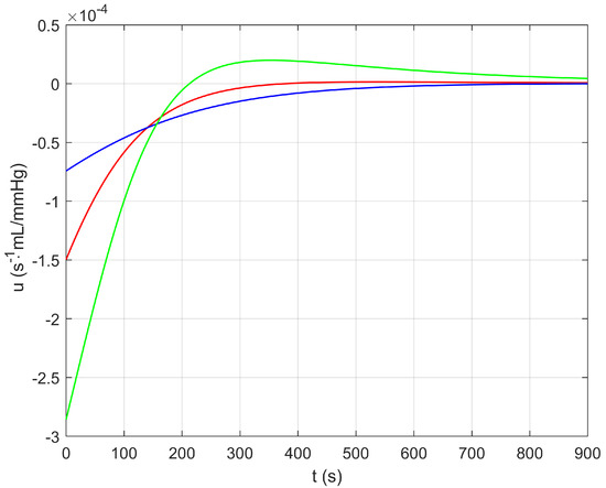
Figure 5. Control input (arterial–arteriolar compliance rate) versus time (solid red line for ${\kappa }_1=0.002$, ${\kappa }_2=0.01$, $M_1=0.1738$, $M_2=3.46\times {10}^{-4}$; solid blue line for ${\kappa }_1=0.002$, ${\kappa }_2=0.005$, $M_1=0.1738$, $M_2=3.46\times {10}^{-4}$; solid green line for ${\kappa }_1=0.003$, ${\kappa }_2=0.01$, $M_1=0.1738$, $M_2=5.19\times {10}^{-4}$).

Figure 6. Sensitivity of arterial–arteriolar blood flow rate q autoregulation response to changes in systemic arterial pressure steady state values (solid red line for a step decrease to $P_a\left(t\right)\equiv 60$ mmHg, ${\kappa }_1=6.5358\times {10}^{-4}$, ${\kappa }_2=0.01$, $M_1=0.6568$, $M_2=4.2969\times {10}^{-4}$; solid blue line for a step decrease to $P_a\left(t\right)\equiv 80$ mmHg, ${\kappa }_1=0.0012$, ${\kappa }_2=0.01$, $M_1=0.2490$, $M_2=3.0474\times {10}^{-4}$; solid green line for a step increase to $P_a\left(t\right)\equiv 120$ mmHg, ${\kappa }_1=0.0019$, ${\kappa }_2=0.01$, $M_1=0.1643$, $M_2=3.0938\times {10}^{-4}$; solid magenta line for a step increase to $P_a\left(t\right)\equiv 140$ mmHg, ${\kappa }_1=0.0023$, ${\kappa }_2=0.01$, $M_1=0.2942$, $M_2=6.7020\times {10}^{-4}$; solid black line for a step increase to $P_a\left(t\right)\equiv 160$ mmHg, ${\kappa }_1=0.0026$, ${\kappa }_2=0.01$, $M_1=0.3984$, $M_2=0.001$; dashed line for the reference value $q=q_n$).

Figure 7. Arterial–arteriolar blood flow rate q autoregulation response (solid black line) to a step systemic arterial pressure increase to $P_a\left(t\right)\equiv 160$ mmHg under ${\kappa }_1=0.0026$, ${\kappa }_2=0.002$, $M_1=0.3984$, $M_2=0.001$ (dashed line for the reference value $q=q_n$).

Figure 6 and Figure 7 illustrate the sensitivity of the arterial–arteriolar blood flow rate q autoregulation response to changes in systemic arterial pressure steady state values. All arterial pressure changes started from the basal steady state value $P_a\left(t\right)\equiv 100$ mmHg.

Notice that the simulation results show the good performance and flexibility of the cerebral blood flow autoregulation scheme (34). By adjusting parameters ${\kappa }_1$, ${\kappa }_2$ and $M_1$, $M_2$ of the control law (33), one can provide medically reasonable transients within required regulation times and bounds. Even if one control parameter set fails to yield satisfactory autoregulation responses for the whole range of arterial blood pressure values $P_a\in [60,160]$ mmHg, as shown in Figure 6, one can readily adjust, e.g., the gain coefficient ${\kappa }_2$, as demonstrated in Figure 7, to obtain reasonable cerebral blood flow autoregulation time behavior.

5. Discussion

In this paper, we proposed to treat the cerebral blood flow autoregulation modeling problem as an output tracking automatic control problem. This is the first time, at least to our knowledge, that the cerebral blood flow lumped parameter model introduced in [4] was studied as a dynamical system with control input and its controllability properties were analyzed. It was shown that the cerebral hemodynamics model in question is differentially flat. This fact reveals good potential for applying a variety of automatic control tools to design the impaired cerebral autoregulation compensation mathematical algorithms. Within the current research, due to the model’s nonlinearity, such a well-known and effective nonlinear control approach as integrator backstepping combined with barrier Lyapunov functions was used to construct the control laws that recover the cerebral autoregulation performance of a healthy human. Additionally, the backstepping-based design in question can be further strengthened to account not only for the model nonlinearities but also for various model uncertainties; see, e.g., [17].

The cerebral autoregulation model was developed in terms of arterial–arteriolar compliance time behavior in the form of a feedback control law that utilizes information on the intracranial pressure and arterial–arteriolar blood volume time profiles. It is worthwhile to notice that the intracranial pressure and arterial–arteriolar blood volume values are not available for direct measurements during clinical maneuvers. Hence, future research can be focused on the estimation of the unmeasured quantities using, e.g., state observer construction techniques [20] based on measurements of the arterial–arteriolar blood flow rate values.

References

- Hambleton, G.; Wigglesworth, J.S. Origin of intraventricular haemorrhage in the preterm infant. Arch. Dis. Child. 1976, 51, 651–659. [Google Scholar] [CrossRef] [PubMed] [Green Version]
- Volpe, J.J. Neurology of the Newborn; Elsevier Health Sciences: Amsterdam, The Netherlands, 2008. [Google Scholar]
- Paulson, O.B.; Strandgaard, S.; Edvinsson, L. Cerebral autoregulation. Cerebrovasc. Brain Metab. Rev. 1990, 2, 161–192. [Google Scholar] [PubMed]
- Ursino, M.; Lodi, C.A. A simple mathematical model of the interaction between intracranial pressure and cerebral hemodynamics. J. Appl. Physiol. 1997, 82, 1256–1269. [Google Scholar] [CrossRef] [PubMed]
- Olufsen, M.S.; Nadim, A.; Lipsitz, L.A. Dynamics of cerebral blood flow regulation explained using a lumped parameter model. Am. J. Physiol. Regulatory Integrative Comp. Physiol. 2002, 282, R611–R622. [Google Scholar] [CrossRef] [PubMed] [Green Version]
- Spronck, B.; Martens, H.J.; Gommer, E.D.; Vosse, F.N. A lumped parameter model of cerebral blood flow control combining cerebral autoregulation and neurovascular coupling. Am. J. Physiol. Heart Circ. Physiol. 2012, 303, H1143–H1153. [Google Scholar] [CrossRef] [PubMed] [Green Version]
- Lampe, R.; Botkin, N.; Turova, V.; Blumenstein, T.; Alves-Pinto, A. Mathematical modelling of cerebral blood circulation and cerebral autoregulation: Towards preventing intracranial hemorrhages in preterm newborns. Comp. Math. Meth. Med. 2014, 2014, 965275. [Google Scholar] [CrossRef] [PubMed]
- Botkin, N.; Turova, V.; Lampe, R. Feedback control of impaired cerebral autoregulation in preterm infants: Mathematical modelling. In Proceedings of the 25th Mediterranean Conference on Control and Automation (MED), Valletta, Malta, 3–6 July 2017; pp. 229–234. [Google Scholar]
- Botkin, N.D.; Kovtanyuk, A.E.; Turova, V.L.; Sidorenko, I.N.; Lampe, R. Direct modeling of blood flow through the vascular network of the germinal matrix. Comput. Biol. Med. 2018, 92, 147–155. [Google Scholar] [CrossRef] [PubMed]
- Botkin, N.D.; Kovtanyuk, A.E.; Turova, V.L.; Sidorenko, I.N.; Lampe, R. Accounting for tube hematocrit in modeling of blood flow in cerebral capillary networks. Comp. Math. Meth. Med. 2019, 2019, 4235937. [Google Scholar] [CrossRef] [PubMed]
- Payne, S. Cerebral Autoregulation. Control of Blood Flow in the Brain; Springer: Berlin/Heidelberg, Germany, 2016. [Google Scholar]
- Botkin, N.; Turova, V.; Diepolder, J.; Bittner, M.; Holzapfel, F. Aircraft control during cruise flight in windshear conditions: Viability approach. Dyn. Games Appl. 2017, 7, 594–608. [Google Scholar] [CrossRef] [Green Version]
- Fliess, M.; Lévine, J.; Martin, P.; Rouchon, P. Flatness and defect of non-linear systems: Introductory theory and examples. Int. J. Contr. 1995, 61, 1327–1361. [Google Scholar] [CrossRef] [Green Version]
- Chetverikov, V.N. Controllability of flat systems. Diff. Eq. 2007, 43, 1558–1568. [Google Scholar] [CrossRef]
- Isidori, A. Nonlinear Control Systems, 3rd ed.; Springer: Berlin/Heidelberg, Germany, 1995. [Google Scholar]
- Rangel-Castilla, L.; Gopinath, S.; Robertson, C.S. Management of intracranial hypertension. Neurol. Clin. 2008, 26, 521–541. [Google Scholar] [CrossRef] [PubMed]
- Krstić, M.; Kanellakopoulos, I.; Kokotović, P.V. Nonlinear and Adaptive Control Design; John Wiley and Sons: Hoboken, NJ, USA, 1995; p. 563. [Google Scholar]
- Ngo, K.B.; Mahony, R.; Jiang, Z.P. Integrator backstepping using barrier functions for systems with multiple state constraints. In Proceedings of the 44th IEEE Conference on Decision and Control, and the European Control Conference, Seville, Spain, 12–15 December 2005; pp. 8306–8312. [Google Scholar]
- Khalil, H.K. Nonlinear Systems, 3rd ed.; Prentice Hall: Hoboken, NJ, USA, 2002. [Google Scholar]
- Besançon, G. Nonlinear Observers and Applications; Springer: Berlin/Heidelberg, Germany, 2007. [Google Scholar]
Publisher’s Note: MDPI stays neutral with regard to jurisdictional claims in published maps and institutional affiliations. |
© 2022 by the authors. Licensee MDPI, Basel, Switzerland. This article is an open access article distributed under the terms and conditions of the Creative Commons Attribution (CC BY) license (https://creativecommons.org/licenses/by/4.0/).