Abstract
In this article, we solve fractional Integro differential equations (FIDEs) through a well-known technique known as the Chebyshev Pseudospectral method. In the Caputo manner, the fractional derivative is taken. The main advantage of the proposed technique is that it reduces such types of equations to linear or nonlinear algebraic equations. The acquired results demonstrate the accuracy and reliability of the current approach. The results are compared to those obtained by other approaches and the exact solution. Three test problems were used to demonstrate the effectiveness of the proposed technique. For different fractional orders, the results of the proposed technique are plotted. Plotting absolute error figures and comparing results to some existing solutions reveals the accuracy of the proposed technique. The comparison with the exact solution, hybrid Legendre polynomials, and block-pulse functions approach, Reproducing Kernel Hilbert Space method, Haar wavelet method, and Pseudo-operational matrix method confirm that Chebyshev Pseudospectral method is more accurate and straightforward as compared to other methods.
Keywords:
Chebyshev Pseudospectral method (CPM); fractional integro-differential equations; caputo operator MSC:
26A33; 47G20; 37N30
1. Introduction
Fractional calculus (FC) deals with derivatives and integrals of an arbitrary order (real or complex order). The history of FC started from 30 September 1695, when Leibnitz described a derivative of order (see [1]). In the 19th century, Riemann and Liouville defined the concept of differentiation to an arbitrary order (fractional differentiation). However, there were few specific models based on this type of derivative at that time due to which the study of fractional order systems attracted little interest. Nowadays, a growing number of researchers are focusing their attention on FC, and they have shown that fractional systems can retain information that is missing in integral order systems. Scientists pay more attention to FC due to its numerous applications in many areas such as solid mechanics [2], oscillation of earthquakes [3], signal processing [4], economics [5], electrode-electrolyte polarization [6], control theory [7], visco-elastic materials [8], and continuum and statistical mechanics [9]. Fractional derivatives can be described in different ways, e.g., Grünwald Letnikow, Caputo, and Generalized Functions Approach. In the present article, we focus on Caputo’s derivative, which is more useful in real-life applications [10,11,12].
In recent years, much attention has been given to the solutions of fractional differential and integro-differential equations. FIDEs have many applications in mechanical, nuclear engineering, chemistry, astronomy, biology, economics, potential theory, and electrostatics. In particular cases, the exact solution of such FIDEs may be found only. In many cases, analytical solutions of integro-differential equations are an unwieldy task, so it is required to obtain an efficient approximate solution. Recently, many effective techniques have been presented to solve integro-differential equations having fractional-order. such as Homotopy perturbation transform method [12], Reproducing Kernal Hilbert Space Method (RKHSM) [13,14], Haar Wavelet Method (HWM) [15], Taylor Expansion Method (TEM) [16], Homotopy Analysis Method (HAM) [17], Euler Wavelet Method (EWM) [18], Spline Collocation Method (SCM) [19], Variational Iteration Method (VIM) [20], Laplace Adomian Decomposition Method (LADM) [21], Homotopy Perturbation Method (HPM) [22] and much more [23,24,25,26].
As Chebyshev polynomials [27] are considered to be a known family of orthogonal polynomials with many applications on the interval , they are commonly used in function approximation because of their good properties. S. Nemati et al. [28] implement a spectral method based on operational matrices of the second kind of Chebyshev polynomials to solve FIDEs having weakly singular kernels. M.S. Mahdy et al. [29] used the least squares method aid of third kind shifted Chebyshev polynomials to solve a linear system of fractional integro-differential equations. However, to the best of our knowledge, the solution of FIDEs has done little to adapt these polynomials. In the present study, we solve FIDEs by implementing CPM. By implementing the proposed method, we compared our results with other techniques. We solve FIDEs of the form
having initial and boundary sources;
where and are real constants, represents the fractional derivative in Caputo manner for , G and H are well-defined functions.
The paper is structured as follows. In Section 2, we provide some basic definitions which are further used in current work. In Section 3, the concept of approximation Chebyshev series expansion by means of Caputo derivative is given. The implementation of the Chebyshev collocation approach to solve Equation (1) is presented in Section 4. In Section 5, we solve some problems to clarify the technique’s effectiveness.
2. Preliminaries Concept
Definition 1.
A function is said to be in space if there exists a real number , with , where and it is said to be in space if and only if
Definition 2.
The derivative having fractional-order in Caputo manner is given as:
where represents the derivative order, and represents the lowest integer greater than β with
For the derivative in Caputo sense we have [30]
Here we utilize ceiling function to represent the lowest integer equal to or greater than with In addition, for the Caputo operator becomes similar to integer-order differential operator. Both operation of integer-order and fractional-order differentiation are similar:
where ϕ and ν are constants.
3. Approximation of Chebyshev Series Expansion by Means of Caputo Derivative
The Chebyshev polynomials are explained on the interval, and can be calculated by means of recurrence formulae as [31,32]
where and The Chebyshev polynomial having degree analytical form is defined by [32]
To define Chebyshev shifted polynomials , we take the Chebyshev polynomials over the interval The Chebyshev shifted polynomials are determined by means of the following relation as [32]
also by means of the below recurrence formula:
where and The orthogonality condition is (see [33])
Now, by using the relation,
and Equation (8) to obtain Chebyshev shifted polynomials analytical form for order as:
A function , described in Chebyshev shifted polynomials form as
where the factors , for are determined by
Thus, in practice first -terms are taken and for few , is calculated as
Theorem 1.
The sum of the absolute values of all the omitted coefficients constrains the inaccuracy in approximating by the sum of its first terms. If, however [34]
Thus, for all , m and , we get
Theorem 2.
Assume that and is calculated by the Chebyshev shifted polynomials as in Equation (16). Then [35]
where is defined by
4. Chebyshev Collocation Method
In this part, we implement Chebyshev’s collocation method to solve FIDE (1) having initial and boundary conditions (2) to achieve this goal, we calculated as
By means of Equations (1) and (21) and Theorem 2 we get
Now we collocate (22) at points
The roots of the shifted Chebyshev polynomial are used to find suitable collocation points . To apply the Gaussian integration formula for (23), we use the transformation to convert the to t-interval
Equation (23), for may be rewritten as
On applying the Gaussian integration formula, for we have
where represents the zeros of the Chebyshev polynomial and are the appropriate weights as in [36]. For polynomials with a degree of less than , the correctness of the Gaussian integration formula provides the basis for the above approximation.
We can generate more equations by substituting (19) into initial or boundary conditions. By putting (19) into the boundary conditions (2), we obtain
Equation (25), when combined with equations of initial sources or boundary sources, yields nonlinear algebraic equations that may be solved using Newton’s iterative approach for applying Newton’s iterative method. As a result, the function from (1) can be computed.
5. Applications
In this part, we solved three integro-differential problems having fractional-order and compared the obtained results with other methods. All the computational work was undertaken through MAPLE.
5.1. Problem 1
Let us consider the FIDE of the form [37]
subject to the initial conditions , having accurate solution at .
The behavior of the exact and proposed method results are illustrated in Table 1. Table 2 illustrates the error comparison among CPM, HWM and HLBF which verify that CPM approaches fast as compared to HWM and HLBF. The solution at different fractional-orders for problem 1 is given in Table 3 which shows that the solution gets closer towards an accurate result as the value of goes from fractional-order towards integer-order. The graphical view for the exact and proposed method solution are given in Figure 1, whereas Figure 2 illustrates the comparison of given techniques on the basis of error. Figure 3 shows the graphical representation of problem 1 at different fractional-orders. It is observed from the results that CPM solutions are in good agreement with the exact solution as compared to HWM and HLBF.

Table 1.
Comparison of the exact and proposed method results with the aid of absolute error for problem 1.
Table 2.
Comparison of the proposed method with other techniques on the basis of absolute error (A.E) for problem 1.
Table 3.
Comparison of the proposed technique solution at various fractional-orders of for problem 1.
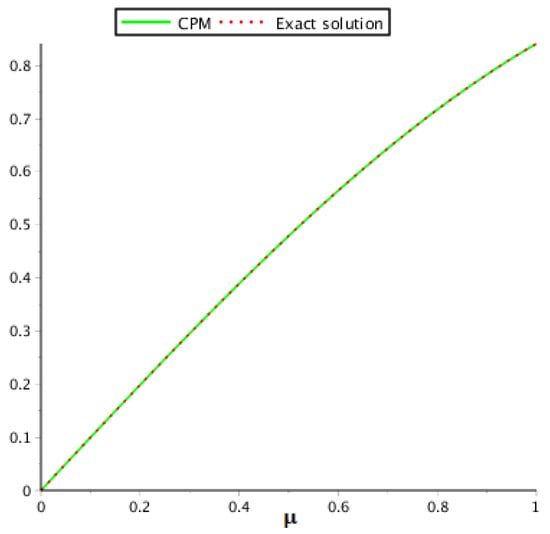
Figure 1.
Analysis of the exact and our method result for problem 1.
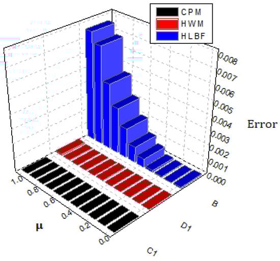
Figure 2.
Comparison of proposed method solution with other methods on error base for problem .
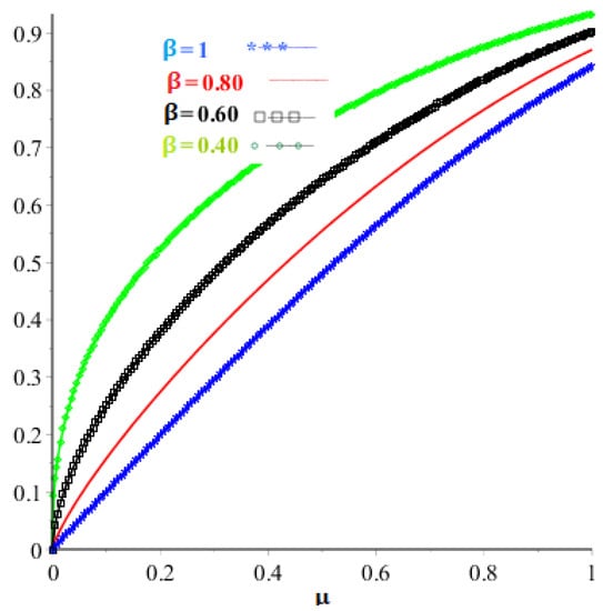
Figure 3.
Analysis of the proposed method solution at various fractional-orders for problem .
5.2. Problem 2
Let us consider the FIDE of the form [38]
subject to the initial sources .
At the accurate solution of the problem is The behavior of the exact and proposed method results are demonstrated in Table 4. Table 5 demonstrates the proposed method and RKHSM error comparison verify that CPM approaches fast as compared to RKHSM, whereas Table 6 shows the behavior of the proposed method at different fractional-orders of problem 2. The graphical view for the exact and proposed method solution are given in Figure 4, while Figure 5 illustrates the comparison of the given techniques on the basis of error. In addition, Figure 6 provides the graphical layout for problem 2 at various fractional-orders. The results we obtained by implementing the proposed technique are better than those of RKHSM.
Table 4.
Comparison of the exact and proposed method results with the aid of absolute error for problem 2.
Table 5.
Comparison of the proposed technique with other technique on the basis of absolute error (A.E) for problem 2.
Table 6.
Comparison of the proposed technique solution at various fractional-orders of for problem 2.
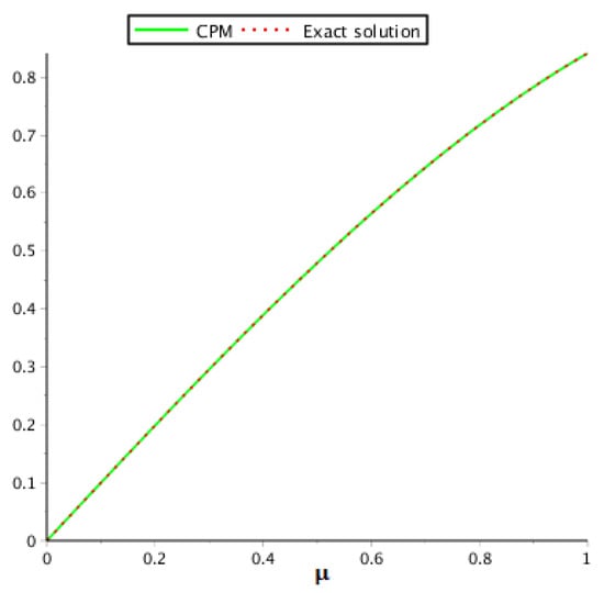
Figure 4.
Analysis of the exact and our method solution for problem 2.
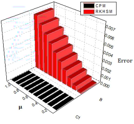
Figure 5.
Comparison of proposed method solution with other method on error base for problem .
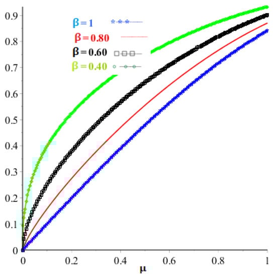
Figure 6.
Analysis of the proposed method solution at various fractional-orders for problem .
5.3. Problem 3
Let us consider the FIDE of the form [39]
with initial sources .
The exact solution of this equation for is . The behavior of the accurate and proposed method result are given in Table 7. Table 8 shows the behavior of the proposed method at different fractional-orders of problem 3. In addition, Table 9 shows the proposed method and POMM error comparison which verify that CPM approaches fast as compared to POMM. The graphical view for the exact and proposed method solution are given in Figure 7, whereas the graphical layout for problem 3 at various fractional-orders is shown in Figure 8.
Table 7.
Comparison of the exact and proposed method solution with the aid of absolute error for problem 3.
Table 8.
Comparison of the proposed technique solution at various fractional-orders of for problem 3.
Table 9.
Comparison of the proposed technique with other technique on the basis of absolute error (A.E) for problem 3.
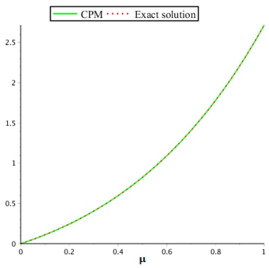
Figure 7.
Analysis of the exact and our method result for problem 3.
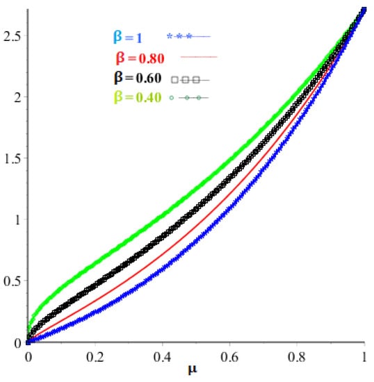
Figure 8.
Analysis of the proposed method solution at various fractional-order for problem .
6. Conclusions
We used the Chebyshev Pseudospectral approach for solving fractional integro-differential equations in this article. In the Caputo manner, the fractional derivative is considered. To reduce fractional integro-differential equations to algebraic equations, the properties of Chebyshev polynomials were combined with the Gaussian integration method which is solved using either the conjugate gradient approach or the Newton iteration approach. Studying the convergence analysis and estimating an upper bound of the error of the resulting formula receives special emphasis. The results obtained by employing the suggested technique are in great agreement with the actual solution and show greater accuracy as compared to other techniques. Furthermore, it is clear from the figures that the proposed method error converges quickly when compared to other approaches. MAPLE was used to perform the calculations in this article.
Author Contributions
Data curation, T.S.H.; Formal analysis, T.S.H.; Funding acquisition, W.W.; Methodology, I.O.; Project administration, R.S.; Resources, I.O. and W.W.; Supervision, W.W.; Writing—original draft, R.S. All authors have read and agreed to the published version of the manuscript.
Funding
This research received no external funding.
Institutional Review Board Statement
Not applicable.
Informed Consent Statement
Not applicable.
Data Availability Statement
The numerical data used to support the findings of this study are included within the article.
Conflicts of Interest
The authors declare that there are no conflict of interest regarding the publication of this article.
References
- Loverro, A. Fractional Calculus: History, Definitions and Applications for the Engineer; Rapport Technique; Univeristy of Notre Dame, Department of Aerospace and Mechanical Engineering: Notre Dame, IN, USA, 2004; pp. 1–28. [Google Scholar]
- Rossikhin, Y.A.; Shitikova, M.V. Applications of Fractional Calculus to Dynamic Problems of Linear and Nonlinear Hereditary Mechanics of Solids. Appl. Mech. Rev. 1997, 50, 15–67. [Google Scholar] [CrossRef]
- He, J.H. Nonlinear oscillation with fractional derivative and its applications. In Proceedings of the International Conference on Vibrating Engineering, Dalian, China, 6–9 August 1998; Volume 98, pp. 288–291. [Google Scholar]
- Baskin, E.; Iomin, A. Electro-chemical manifestation of nanoplasmonics in fractal media. Cent. Eur. J. Phys. 2013, 11, 676–684. [Google Scholar] [CrossRef][Green Version]
- Baillie, R.T. Long memory processes and fractional integration in econometrics. J. Econom. 1996, 73, 5–59. [Google Scholar] [CrossRef]
- Deng, W.H.; Li, C.P. Chaos synchronization of the fractional Lü system. Phys. A Stat. Mech. Its Appl. 2005, 353, 61–72. [Google Scholar] [CrossRef]
- Khan, H.; Farooq, U.; Shah, R.; Baleanu, D.; Kumam, P.; Arif, M. Analytical Solutions of (2+Time Fractional Order) Dimensional Physical Models, Using Modified Decomposition Method. Appl. Sci. 2019, 10, 122. [Google Scholar] [CrossRef]
- Bagley, R.L.; Torvik, P.J. Fractional calculus in the transient analysis of viscoelastically damped structures. AIAA J. 1985, 23, 918–925. [Google Scholar] [CrossRef]
- Mainardi, F. Fractional calculus: Some basic problems in continuum and statistical mechanics. arXiv 2012, arXiv:1201.0863. [Google Scholar]
- Nonlaopon, K.; Naeem, M.; Zidan, A.; Shah, R.; Alsanad, A.; Gumaei, A. Numerical Investigation of the Time-Fractional Whitham–Broer–Kaup Equation Involving without Singular Kernel Operators. Complexity 2021, 2021, 1–21. [Google Scholar] [CrossRef]
- Areshi, M.; Khan, A.; Shah, R.; Nonlaopon, K. Analytical investigation of fractional-order Newell-Whitehead-Segel equations via a novel transform. AIMS Math. 2022, 7, 6936–6958. [Google Scholar] [CrossRef]
- Shah, N.A.; Alyousef, H.A.; El-Tantawy, S.A.; Shah, R.; Chung, J.D. Analytical Investigation of Fractional-Order Korteweg-De-Vries-Type Equations under Atangana-Baleanu-Caputo Operator: Modeling Nonlinear Waves in a Plasma and Fluid. Symmetry 2022, 14, 739. [Google Scholar] [CrossRef]
- Bushnaq, S.; Momani, S.; Zhou, Y. A reproducing kernel Hilbert space method for solving integro-differential equations of fractional order. J. Optim. Theory Appl. 2013, 156, 96–105. [Google Scholar] [CrossRef]
- Akgül, A. Solutions of Integral Equations by Reproducing Kernel Hilbert Space Method. In Topics in Integral and Integro-Differential Equations; Springer: Cham, Switzerland, 2021; pp. 103–124. [Google Scholar]
- Amin, R.; Shah, K.; Asif, M.; Khan, I.; Ullah, F. An efficient algorithm for numerical solution of fractional integro-differential equations via Haar wavelet. J. Comput. Appl. Math. 2021, 381, 113028. [Google Scholar] [CrossRef]
- Huang, L.; Li, X.F.; Zhao, Y.; Duan, X.Y. Approximate solution of fractional integro-differential equations by Taylor expansion method. Comput. Math. Appl. 2011, 62, 1127–1134. [Google Scholar] [CrossRef]
- Abbasbandy, S.; Hashemi, M.S.; Hashim, I. On convergence of homotopy analysis method and its application to fractional integro-differential equations. Quaest. Math. 2013, 36, 93–105. [Google Scholar] [CrossRef]
- Wang, Y.; Zhu, L. Solving nonlinear Volterra integro-differential equations of fractional order by using Euler wavelet method. Adv. Differ. Equ. 2017, 2017, 27. [Google Scholar] [CrossRef]
- Qiao, L.; Wang, Z.; Xu, D. An alternating direction implicit orthogonal spline collocation method for the two dimensional multi-term time fractional integro-differential equation. Appl. Numer. Math. 2020, 151, 199–212. [Google Scholar] [CrossRef]
- Khaleel, O.I. Variational iteration method for solving multi-fractional integro differential equations. Iraqi J. Sci. 2014, 55, 1086–1094. [Google Scholar]
- Ullah, Z.; Ahmad, S.; Ullah, A.; Akgül, A. On solution of fuzzy Volterra integro-differential equations. Arab. J. Basic Appl. Sci. 2021, 28, 330–339. [Google Scholar] [CrossRef]
- Ghazanfari, B.; Ghazanfari, A.G.; Veisi, F. Homotopy perturbation method for nonlinear fractional integro-differential equations. Aust. J. Basic Applid Sci. 2010, 12, 5823–5829. [Google Scholar]
- Akgül, A. A novel method for a fractional derivative with non-local and non-singular kernel. Chaos Solitons Fractals 2018, 114, 478–482. [Google Scholar] [CrossRef]
- Ul Haq, M.; Ullah, A.; Ahmad, S.; Akgül, A. A Quantitative Approach to nth-Order Nonlinear Fuzzy Integro-Differential Equation. Int. J. Appl. Comput. Math. 2022, 8, 1–24. [Google Scholar] [CrossRef]
- Ghanbari, B.; Akgül, A. Abundant new analytical and approximate solutions to the generalized Schamel equation. Phys. Scr. 2020, 95, 075201. [Google Scholar] [CrossRef]
- Modanli, M.; Akgül, A. Numerical solution of fractional telegraph differential equations by theta-method. Eur. Phys. J. Spec. Top. 2017, 226, 3693–3703. [Google Scholar] [CrossRef]
- Alaoui, M.; Fayyaz, R.; Khan, A.; Shah, R.; Abdo, M. Analytical Investigation of Noyes–Field Model for Time-Fractional Belousov–Zhabotinsky Reaction. Complexity 2021, 2021, 1–21. [Google Scholar] [CrossRef]
- Nemati, S.; Sedaghat, S.; Mohammadi, I. A fast numerical algorithm based on the second kind Chebyshev polynomials for fractional integro-differential equations with weakly singular kernels. J. Comput. Appl. Math. 2016, 308, 231–242. [Google Scholar] [CrossRef]
- Mahdy, A.M.; Mohamed, E.M. Numerical studies for solving system of linear fractional integro-differential equations by using least squares method and shifted Chebyshev polynomials. J. Abstr. Comput. Math. 2016, 1, 24–32. [Google Scholar]
- Podlubny, I. Fractional Differential Equations; Academic Press: San Diego, CA, USA, 1999. [Google Scholar]
- Sunthrayuth, P.; Ullah, R.; Khan, A.; Shah, R.; Kafle, J.; Mahariq, I.; Jarad, F. Numerical analysis of the fractional-order nonlinear system of Volterra integro-differential equations. J. Funct. Spaces 2021, 2021, 1537958. [Google Scholar] [CrossRef]
- Kilbas, A.A.; Srivastava, H.M.; Trujillo, J.J. Theory and Applications of Fractional Differential Equations; Elsevier: San Diego, CA, USA, 2006. [Google Scholar]
- Kadem, A.; Baleanu, D. Analytical method based on Walsh function combined with orthogonal polynomial for fractional transport equation. Commun. Nonlinear Sci. Numer. Simul. 2010, 15, 491–501. [Google Scholar] [CrossRef]
- Youssri, Y.H.; Hafez, R.M. Chebyshev collocation treatment of Volterra-Fredholm integral equation with error analysis. Arab. J. Math. 2020, 9, 471–480. [Google Scholar] [CrossRef]
- Khader, M.M. On the numerical solutions for the fractional diffusion equation. Commun. Nonlinear Sci. Numer. Simul. 2011, 16, 2535–2542. [Google Scholar] [CrossRef]
- Constantinides, A. Applied Numerical Methods with Personal Computers; McGraw-Hill, Inc.: New York, NY, USA, 1987. [Google Scholar]
- Aziz, I.; Fayyaz, M. A new approach for numerical solution of integro-differential equations via Haar wavelets. Int. J. Comput. Math. 2013, 90, 1971–1989. [Google Scholar]
- Bushnaq, S.; Maayah, B.; Ahmad, M. Reproducing kernel Hilbert space method for solving fredholm integrodifferential equations of fractional order. Ital. J. Pure Appl. Math. 2016, 36, 307–318. [Google Scholar]
- Dehestani, H.; Ordokhani, Y.; Razzaghi, M. Pseudo-operational matrix method for the solution of variable-order fractional partial integro-differential equations. Eng. Comput. 2021, 37, 1791–1806. [Google Scholar] [CrossRef]


Publisher’s Note: MDPI stays neutral with regard to jurisdictional claims in published maps and institutional affiliations. |
© 2022 by the authors. Licensee MDPI, Basel, Switzerland. This article is an open access article distributed under the terms and conditions of the Creative Commons Attribution (CC BY) license (https://creativecommons.org/licenses/by/4.0/).