1. Introduction
A significant number of experimental and theoretical works are devoted to the study of the structure of jets of combustion products of rocket engines in which, as a rule, the influence of such dimensionless similarity criteria as the Mach number at the nozzle exit and in the cocurrent flow , the adiabatic index , the degree of non-design , Reynolds number and the angle of inclination nozzle contour in the outlet section θa (where is the viscosity coefficient at the nozzle exit, is the longitudinal velocity component at the nozzle exit, is the nozzle exit radius and and are the Mach number and wake pressure at infinity).
Thanks to these studies, it was established that when a supersonic jet flows into a cocurrent supersonic flow, a complex flow structure is formed: hanging barrel-shaped shock waves appear in the external flow and inside the jet, rarefaction waves arise inside the jet, and an expanding mixing layer is formed at the outer boundary of the jet. In this case, the gaseous medium into which the outflow occurs can be at rest relative to the solid propellant rocket engine SFRE (outflow into the flooded space) or move relative to it at a speed (interaction with a cocurrent flow). An increase in pressure leads to the appearance of an initially oblique hanging shock at the nozzle exit, and at a higher counterpressure, the appearance of a Y-shaped system of shocks, consisting of two oblique and one direct shocks, is observed. At a certain threshold value of pressure, the . Y-shaped system of shocks enters the nozzle, separating the boundary layer from the nozzle wall and significantly changing the gas-dynamic flow inside the nozzle apparatus.
It is important to note here that the described picture of the gas flow inside the nozzle apparatus is observed when the gas jet flows into the flooded space and can change under conditions of interaction with the external gas flow. Due to the difference in flow rates in the outgoing jet and the cocurrent flow, a central zone of reverse currents appears, which has a toroidal shape. The size and location of the reverse flow zones strongly affect the performance of the solid propellant rocket engine combustion chambers, which requires appropriate research.
In addition, this paper also considers the issue of the impact of a shock wave resulting from the impact on the oncoming undisturbed supersonic air flow of the head part of a solid propellant rocket engine on the thermal physical parameters of the cocurrent air jet and combustion products flowing from the nozzle apparatus of a solid-fuel rocket engine.
The paper presents a theoretical model of a solid fuel rocket, which allows calculating the characteristics of gas-dynamic processes in the nozzle block of a solid fuel rocket engine (SFRE) as well as calculating the interaction of the combustion product jet with the surrounding gas medium based on a unified numerical methodology. The computational studies are carried out within the framework of viscous (Navier–Stokes equations) gas flow. Earlier multigrid methods have been created, and the computation for convection–diffusion equations on nonuniform grids and equations with dynamic boundary conditions was performed. Numerical simulations have been developed for different flows and aerodynamic applications [
1,
2,
3].
The important point in the numerical modeling of Navier–Stokes equations is the construction of a computational grid in complicated two- and three-dimensional domains Ω, which represents the computational domain Ω in the form of separate finite elements (cells). In this paper, the hexagonal irregular grid method, based on the hybrid non-structural multi-block structuring grids, is used for such domains. For this purpose, uniform partitioning of the domain into rectangular cells of size , and the boundary of the computational domain Ω is presented as a piecewise-smooth contour consisting of curvilinear segments approximated by Bezier curves, is applied as an initial approximation. The numerical technique used in this research makes it possible to construct nonorthogonal structured grids even in those areas where non-structured computational grids are normally used to discretize the computational domain.
2. Method for Constructing Adaptive Grids
It is known from practical calculations that structured computational grids are preferable for solving problems in plasma dynamics and aerodynamics. However, the range of technical objects, the surface geometry of which can be described by structured computational grids, is rather limited. Therefore, there is a compromise option—a hybrid unstructured block-tetrahedral computational grid.
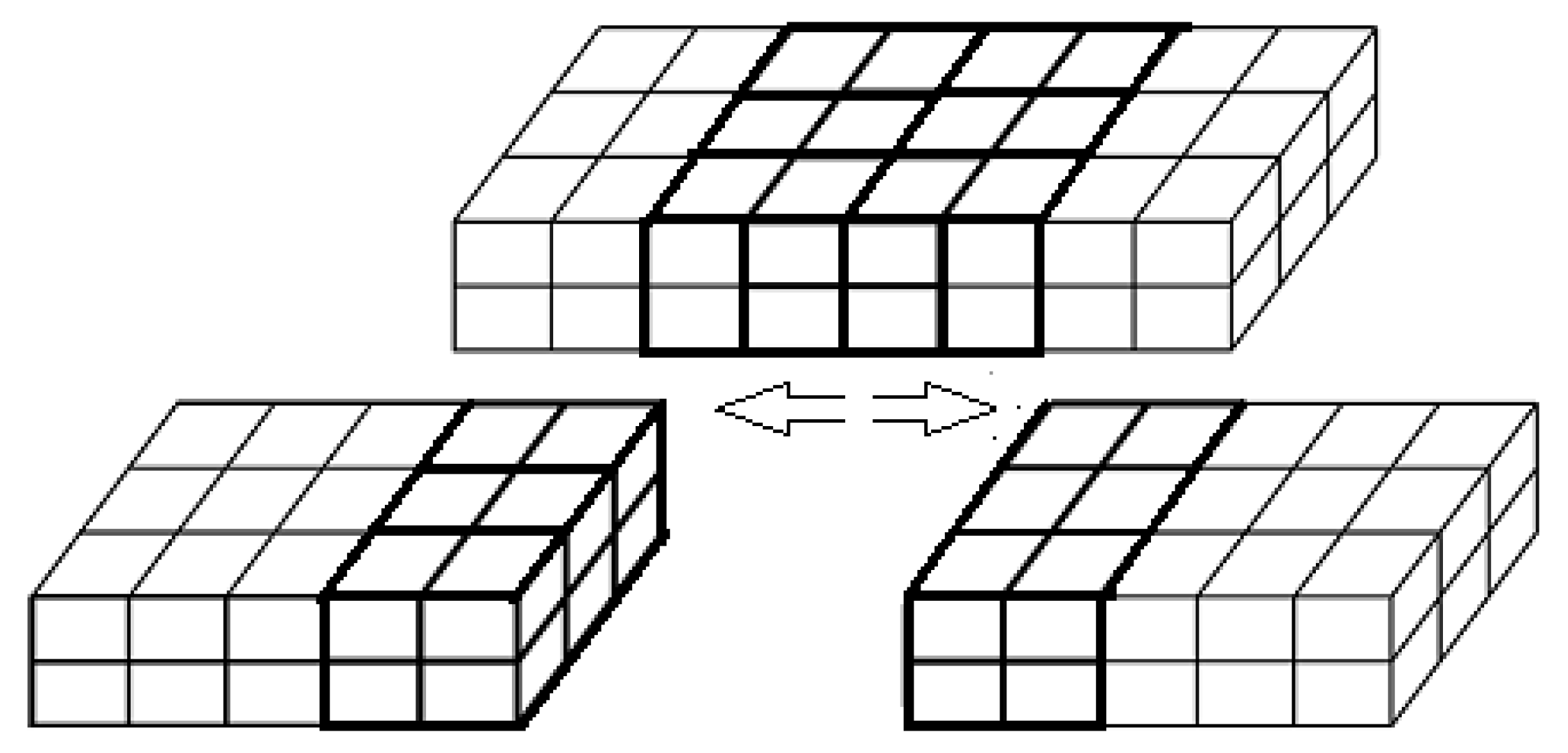
The use of a complex block-structured grid involves shaping the geometry of the computational domain by representing it as a group of hexahedral block-primitives (
Figure 1), each of which constructs its structured grid
consistent with the grid in neighbouring blocks. The implementation of this approach requires that the blocks-primitives are docked on the boundaries with each other, and the computational grid formed in each block is combined into a single unstructured grid with common node numbering (
Figure 2).
To approximate the curvilinear surfaces of faces, a Bezier projective surface is used, which is defined by a finite set of ordered points of three-dimensional space called the matrix of poles and the matrix of weights assigned to the same points. By changing the positions of the poles (control points) and the values of weights , we can control the closeness of the shape of the Bezier projective surface to the shape of the smooth curvilinear surfaces of the faces. Note here that the larger (relative to other points) the value of the weighting factor , the closer the Bezier surface is to the corresponding point on the face surface of the primitive block (decreasing the weight of the vertex will have the opposite effect).
Analytically, a Bezier projective surface of order
n ×
m (its representation is related to Bernstein basis polynomials
,
) is described by a fractional-rational function
of the following form (the weights
of the angular vertices are considered to be equal to 1):
where
,
are the binomial coefficients, and
is the pole matrix consisting of vectors (with x, y, z components) of control points.
When writing this formula, it is assumed that there is a set of control points conventionally arranged as n + 1 rows of m + 1 points in each row. The indices of point mean that the given j-th control point is located in the i-th row (the first index equals the number of the row; the second index equals the number of the point in the row). Note also that the expression for is a convex hull of the poles . That is, the projective Bezier surface will be located inside this convex hull, “stretched” on these poles.
The Bezier surface can (for the convenience of further calculations) be written in vector form:
where
,
,
.
Let us assume that on any curvilinear face surface,
N ×
M points are interpolation nodes, for which their Cartesian
(
) coordinates are known (as well as their corresponding values of parameters
), listed in the order of their connection in the framework of control points of the face being constructed. Then using the coordinate values of the interpolation nodes
(and
) and the formula for
, we can formulate a system of linear equations with the unknowns being the coordinates of the control points (the pole matrix
):
where
is a number of interpolation nodes on the curvilinear face;
is the number of unknowns for each component (
x,
y or
z) of pole matrix
;
is its radius vector; the Cartesian coordinates of points (in number
) on the curvilinear face are approximated by the Bezier surface; and
are parameter values (with a changing area
), appropriate to specified points
, where
, on the curvilinear face.
However, such a system of equations will in most cases be overdetermined. The least squares method [
4] can be used to overcome this disadvantage:
where
is the number of interpolation nodes on the curvilinear face;
is the number of unknowns for each component (
x,
y or
z) of pole matrix
;
are its radius vector and Cartesian coordinates of points (in number
) on the curvilinear face, which is approximated by the Bezier surface; and
are parameter values (with a changing area
), appropriate to specified points
, where
on the curvilinear face.
Using the found projective variant (Bezier surface) of each curvilinear surface of block-primitive faces, a surface grid of block-primitives can be constructed. Then operating on this surface grid and using the method of three-dimensional transfinite interpolation [
5] as well as the quasi orthogonalization method, a bulk structured quasiorthogonal computational grid (consisting of grid surfaces whose nodes are numbered using parameters) inside the block-primitive is created. Then, as mentioned above, the constructed local (in block-primitive) computational grid is combined (
Figure 3) into a single global unstructured grid with common node numbering. After that, an additional stage of its optimization (improvement—“regularization”) with the assessment of its quality is applied.
For numerical adaptation (to the solution peculiarities) of the volumetric computational grid, the results of [
6] or the principle of uniform distribution (equidistributional method) of the “adaptation” (weight) function
w are used.
To give the bulk structured computational grid (generally speaking non-orthogonal) inside the block-primitive properties of quasiorthogonality, an approximate solution of the equation describing the longitudinal deformation of the plates is found in [
7]. The initial approximation for the mock orthogonalization method is the computational grid obtained after the numerical adaptation step.
When describing the mock orthogonalization method, we introduce in the Cartesian coordinate system XYZ a rectangular parallelepiped , which has a continuously differentiable way to be mapped into a curvilinear parallelepiped (hexahedron) . The rectangular grid mapped to the domain forms , a smooth curvilinear grid in the domain .
Denote by
the radius vector in the
XYZ coordinate system and introduce a vector
characterizing the displacement of points. Here,
and
are radius vectors of points of domains before
and after
transformation. To construct regular adaptive grids close to being orthogonal, the following equations are used to determine the displacement values
and to describe the longitudinal deformation of the plates [
7]:
The boundary conditions required to solve this system of equations are given as follows: , , where the symbol ∂ means that the components of the radii of the vectors and are defined at the boundary of the corresponding domain.
The components of the covariant and contravariant metric tensor entering the system of equations are defined by the relations:
The coefficient describes the ratio of transverse strain to longitudinal strain. The coefficient is a control function used to achieve the desired degree of densification of the grid lines in the area of the strongest change in gas-dynamic functions or spatial boundaries.
Let us introduce vectors
tangent to the grid lines in the spatial domain
; then the control function can be formulated in the form
This kind of control function leads to the orthogonalization of relatively small cells. In the numerical construction of high aspect ratio grids, instead of contour integrals, the sum of expressions of the form or , etc., and overall grid corners will be used.
To solve the problem
, we used the method of establishment [
8]. Step by “time”
is found using the iterative method of a variational type.
3. A Mathematical Model for Determining the Individual Characteristics of a Solid-Propellant Rocket
This section considers the effect of a ballistic wave, resulting from the oncoming unperturbed airflow of the monoblock head part, on the thermophysical parameters of the down jet of air and combustion products flowing from the nozzle of a solid fuel rocket engine.
The numerical investigations of such kinds of flows can be performed on the basis of the solution of Navier–Stokes equations. The case of transition from Cartesian coordinates
to arbitrary curvilinear coordinates
while taking into account the absence of dependence of this transformation on time
is used for transformation. In this case, the system of Navier–Stokes equations of a compressible heat-conducting gas in arbitrary curvilinear coordinates
takes the form [
9]:
where
,
and
T are pressure, density and temperature;
and
are internal and kinetic energies of gas;
is stress tensor;
is the contravariant metric tensor;
is the contravariant components of the velocity vector,
;
is the shear viscosity; and
is the heat transfer coefficient. In these expressions, repeated indices summation is assumed.
The reduced system of equations is supplemented by the initial conditions:
The boundary conditions that determine the characteristics of the combustion products entering the engine chamber from the surface of a burning solid fuel have the form:
where
,
,
,
and
R are the speed, density, temperature, internal energy and gas constant of incoming gaseous combustion products from the surface of solid fuel;
is the density of solid fuel; and
is the speed of movement of the surface of the fuel during its burnout. It is assumed that gas injection into the engine chamber occurs along the normal to the fuel surface. The burnup rate is known from experimentation or from calculations of the combustion kinetics [
10]. It is given in the following form [
11]:
where
is the value of the speed of movement of the burnable fuel boundary at pressure
P = 1, and
v is the constant, depending on the type of fuel used.
On the stationary solid surfaces of the nozzle and the front bottom of the engine, the conditions of impermeability are set as . At the boundary of the computational domain (behind the nozzle exit), through which the co-flow enters, the following gas-dynamic parameters are set: , where , and are the velocity, density and pressure of the gas entering through the boundary surface, respectively.
On the external (located at sufficiently large distances from the nozzle exit) surfaces of the computational domain, the free flow conditions are set as where is the coordinate normal to the boundary surface, and is the vector of resulting variables.
Given what is known in the physical space,
coordinates of the grid nodes in the computational domain
, the metric coefficients can generally be found by numerical differentiation using the formulas [
12].
The Christoffel symbols of the second kind are found using the formula , and for the case of Euclidean physical space , also using the formula .
4. Computational Method
To solve the gas-dynamic part of the system of equations, a nonlinear quasimonotone compact-polynomial difference scheme of higher-order accuracy [
7,
13,
14,
15], as well as a spatial splitting of Navier–Stokes equations [
7] written in an arbitrary curvilinear coordinate system, were used. To calculate the flux vectors at the boundaries of the computational cell, the discontinuity calculation procedure formulated in [
16] was applied. Other details of the nonlinear quasi-monotone compact polynomial difference scheme are given in [
7,
13]. The time step required to integrate the above difference scheme was chosen from the condition of the Courant–Friedrichs–Levy stability criterion.
The “hyperbolic” (convective) part of the computer model of targets was tested on a one-dimensional version of the Riemann problem (Soda problem) about the decay of an unstable discontinuity of a given configuration. A comparison of the exact solution and the approximate solution showed that the difference is not more than one percent [
16]. Verification calculations were carried out to estimate the degree of attenuation of the reflected shockwave system and showed that the calculation error is within the experimental accuracy of the results and can reach a level of 10%. As an additional verification test, we considered flowing air around a wedge mated to a plate and a cone mated to a cylinder with the following oncoming flow parameters: pressure P = 2060 Pa, speed V = 1860 m/s, temperature
T = 223 K and Mach number
. These results are also in good agreement [
12] with the above calculations (relative error of 0.4%). In addition, the methodology was tested with an example of a viscous jet flowing into a downstream gas stream [
17] (relative error of 5%). The “thermal” (“parabolic”) part of the model has been tested on some problems admitting exact analytical solutions: heating of a continuous medium [
18] filling a flat semibounded space
by a heat flow through the left fixed boundary
(relative error less than 1.0%).
A composite two-block structured grid was invented, which was combined into a single computational grid. Block number one of the computational grid described the grid space of the combustion chamber, the nozzle block and the wake jet of combustion products. The characteristic size of the computational grid in the first block is 150 × 400 cells. The second block is located outside the solid propellant rocket monoblock and the wake (these two blocks are separated (for illustration) from each other by a black line in
Figure 4,
Figure 5 and
Figure 6). The characteristic size of the computational grid in this block is 350 × 550 cells. The calculation cells were thickened in the area of the boundary layer (the thickness of the boundary layer is several millimeters; the number of cells in the direction perpendicular to the SFRE surface is not less than 50) in the head part of the monoblock, at the cut of the combustion chamber nozzle and also in the mixing layers. The density gradient was used as a control (monitor) function.
5. Some Results of Calculations of Gas-Dynamic Parameters of a Jet Flowing into a Downstream Gas Stream
Based on the developed numerical codes [
19,
20,
21] a numerical simulation of two trajectory points of the ARIAN 5 missile flight path was carried out: (1)
W∞ = 0.72 km/s,
P∞ = 0.036 at,
T∞ = 270 K, γ = 1.4, distance from the Earth’s surface 25 km and (2)
W∞ = 1.5 km/s,
P∞ = 0.00065 at,
h = 55 km). The prototype engine chosen was the solid propellant rocket engine P-85, which belongs to the medium class of solid propellant boosters of the European Space Agency [
22], i.e., the monoblock consists of a cylinder with length
Znoz = 1060 cm, diameter equal to the diameter of the nozzle shear
Dnoz = 215 cm and a conical head with an opening angle of 54 degrees. The condensed phase was neglected [
23].
Figure 4 and
Figure 5 show the spatial distributions of temperature
and Mach numbers for the first and second points of the trajectory of the ARIAN 5 rocket. The following notations were used: Mach numbers at nozzle cutoff
= 4 and in unperturbed flow
, adiabatic exponent
and degree of inconsistency
(where the indices a and ∞ correspond to the gas-dynamic parameters at nozzle cutoff and unperturbed flow).
Figure 4 shows spatial distributions of the temperature and Mach number corresponding to the first point of the monoblock flight path. In this case, a flow pattern corresponding to a small value of the degree of inconsistency (
h = 25 km,
n = 1) was realized. Here, due to a sufficiently large value of pressure in the down jet (
P∞ ≈
Pa), the radial expansion of the central exhaust gas jet was strongly limited. This limitation lead to the falling of the densification jump on the jet axis (axial coordinate of drop region
Z = 1700 cm—conic nozzle shape) with the following regular reflection from it; the temperature distribution was aligned along the jet axis, and the characteristic transverse size of the central jet was close to diameter of nozzle shear. In this case, the number of “barrels” increases (if we compare with the results of 55 km) and becomes more than one during interaction between the down jet and the central jet.
At high under-expanding (second point of the flight path; option
h = 55 km,
n = 80), the flow pattern shown in
Figure 5 is realized. These figures illustrate the wave structure of a highly under-expanded jet flow into the cocurrent stream. From the given distributions, it can be seen that with sufficiently high values of the degree of under-expansion n near the exit edge of the nozzle and in the down jet of ambient air due to the collision of the expanding jet of the SFRE exhaust and the down jet, an oblique shock wave (SW) and a hanging SW falling on the jet axis, which is characterized by a regular reflection from the jet axis (the axial coordinate of the incident area
Z = 1700 cm—“conical” nozzle shape), emerge. In this case, due to the fact that the size of the first barrel grows as
, only the first “barrel” is observed, the size of which significantly exceeds the characteristic transverse size of the SFRE.
The calculations also show that there is a noticeable (second trajectory point in
Figure 5) effect of the leading shock wave on the thermophysical parameters of the down jet of air and combustion products expiring from the nozzle of the solid propellant rocket engine.
It is known [
24,
25,
26,
27,
28] that a decrease in the degree of non-design
n below a certain value
ncr leads to the irregular reflection of the incident shock from the jet axis with the formation of a
Y-shaped system of shocks, consisting of two oblique and one direct shocks. Spatial distributions of the Mach number, pressure and longitudinal velocity in combustion products and wake air corresponding to the first point of the ARIAN 5 flight trajectory (flight altitude 6 km), which are presented in
Figure 6 and
Figure 7, illustrate this fact. In this group of calculations, the formation of “barrels” is not observed; the temperature along the jet axis is equalized and amounts to 600 K. The decrease in the degree of non-design is accompanied by an irregular reflection of the hanging shock from the jet axis with the formation of a figurative system of shocks, consisting of two oblique and one direct shocks. In these variants of calculations (altitude 6 km, degree of non-design
n = 0.7), this shock system had a “standard” form, entered the supersonic part of the nozzle and led to the separation of the SFRE exhaust gas flow from the nozzle walls. At the same time, a zone of reverse currents formed behind the central shock wave, which has a toroidal shape [
29].
The appearance of the reverse flow zone is mainly associated with a large positive pressure gradient (
Figure 7, axial region (
cm)) behind the nozzle exit [
24], which occurs due to a sharp expansion of the wake jet towards the axis of the coaxially interacting jets (the pressure in the wake jet
is approximately twice the pressure at the nozzle exit
).
Wake jet expansion leads to the narrowing and hence the deceleration (with pressure increase to
; see
Figure 7) of the jet flowing out through the solid propellant rocket nozzle exit, consisting of combustion products. This increase in pressure creates a positive gradient in the axial region (
cm), which leads to the occurrence of a reverse flow (
Figure 7, for
Z = 1000 cm,
Vz = −1 × 10
−5 cm/s). At the same time, as can be seen from
Figure 7, the equilibrium condition for the vortex flow is satisfied (the pressure inside the shock system (3); (4) is equal to the flow pressure in the stagnation zone
), and the vortex region spatially fixes its position.
Thus, apparently, a necessary condition for the occurrence of a vortex region in the nozzle apparatus behind the shock wave is the achievement in the stagnation zone (
Figure 7, at
) of the level of pressure values equal to the total pressure in the cocurrent air flow, i.e.,
. In this case, it is also necessary that the degree of non-design
n < 1, determined at the nozzle exit, be located below a certain critical value
ncr.
In general, the structure of the gas flow in the SFRE nozzle block under the condition of the formation of a zone of reverse currents differs from the case of flow, when a Y-shaped system of shocks is formed inside the nozzle, and can be described as follows (
Figure 6): the main shock wave resulting from the entry of a hanging shock wave into the nozzle apparatus; secondary SW or compression wave, which may appear due to the occurrence of a reverse flow at a large value of the positive pressure gradient in the stagnation zone; zone of reverse currents, located behind the system of jumps; and stagnation zone of the flow of combustion products of solid fuel, located behind the nozzle exit and responsible for the occurrence of a positive pressure gradient
P.
The dimensions, shape and location of the reverse current zone are determined by the following factors:
- *
Ratio of velocities in the wake and central jets;
- *
Degree of unaccountability n;
- *
Geometry of the nozzle.


