Simulations of Hypersonic Boundary-Layer Transition over a Flat Plate with the Spalart-Allmaras One-Equation BCM Transitional Model

Abstract

Transitional flow has a significant impact on vehicles operating at supersonic and hypersonic speeds. An economic way to simulate this problem is to use computational fluid dynamics (CFD) codes. However, not all CFD codes can solve transitional flows. This paper examines the ability of the Spalart–Allmaras one-equation BCM (SA-BCM) transitional model to solve hypersonic transitional flow, implemented in the open-source CFD code Eilmer. Its performance is validated via existing wind tunnel data. Eight different hypersonic flow conditions are applied. A flat plate model is built for the numerical tests. The results indicate that the existing SA-BCM model is sensitive to the freestream turbulence intensity and the grid size. It is not accurate in all the test cases, though the transitional length can be matched by tuning the freestream intensity. This is likely due to the intermittency term of the SA-BCM model not being appropriately calibrated for high-velocity flow, though if the model can be recalibrated it may be able to solve the general high-velocity flows. Although the current SA-BCM model is only accurate under certain flow conditions after one calibration process, it remains attractive to CFD applications. As a one-equation model, the SA-BCM model runs much faster than multiple-equation flow models.

1. Introduction

The transition region in fluid dynamics refers to an area where a laminar flow is transforming to turbulent flow, typically in a boundary layer. Due to the difficulty of predicting the onset of transition, the uncertainty of this location can have a significant impact on engineering applications, affecting shock wave/boundary layer interactions, increasing the heat transfer rate, and impacting the separation of shear layers [1,2]. Accurate predictions of this phenomenon are, therefore, critical to the re-entry stage of reusable launch vehicles and scramjet-powered vehicles [3]. Transition also increases uncertainties in the prediction of the aerodynamics of wind turbine blades [4]. Turbulent transition is initiated by noise in the freestream flow, which comes from the surroundings via sound waves or vibrations, and interactions with the flow around an object of interest. Further downstream, the initially small noise gets amplified by instabilities, and eventually can trigger a chaotic turbulent breakdown. There exist many known instabilities, including those producing roughness, waviness, bluntness [5,6]. Other instabilities include Gortler, the first mode, the second mode, 3D cross flow, and the shock layer [7,8,9,10]. However, research into laminar–turbulent transition is often stymied by difficulties with conventional wind tunnel tests. Data can be disturbed by the high level of noise from the wind tunnel walls [5,11]. Furthermore, large differences between conventional-tunnel data and quiet-tunnel data may be expected [5].

To avoid the cost of physical experiments, computational fluid dynamics (CFD) is a popular method of analyzing fluid dynamics; however, the reliability of CFD results mainly depends on the solver types and flow models within. Most conventional turbulent flow models in CFD software (ANSYS 2022 R2; ANSYS, Inc.; Canonsburg, PA, USA, OpenFoam 6/7/8/9/10; The OpenFoam Foundation Ltd.; USA) are adapted from Reynolds-averaged Navier–Stokes (RANS) equations. One-equation models are one type of RANS model, and include the Spalart–Allmaras (SA) model and Bradshaw’s model [12,13]. Two-equation models are another type, such as the $k-\epsilon$ model, $k-\omega$ model, and Menter’s Shear Stress Transport turbulence (SST) model [14,15,16]. The third type includes more complex stress-transport models, such as the Launder–Reece–Rodi (LRR) model [17]. Although these conventional models work well in specific cases, they are unable to predict boundary-layer transitional flow, or model the transition region in an accurate manner [12,13,14,15,16,17,18,19,20,21,22]. It should also be noted that direct numerical simulation (DNS) is able to solve this problem; nevertheless, the cost of computing resources is too high for it to be widely adopted [23,24], at least for engineering applications.

Many researchers have developed modifications of RANS models that work for transitional flow. These modifications draw on an improved understanding of the mechanisms of transition, such as bypass transition, K-type transition, and H-type transition [25,26]. It is known that secondary instability has a major impact on bypass transition, while other types of transition can be predicted by linear stability theory. Recent CFD studies have probed these phenomena using DNS methods [27,28,29]. Additionally, hypersonic boundary-layer transition has been studied by Mee [30] in a shock tunnel, finding that the length of a transition region increases with the flow velocity. In a hypersonic boundary layer, the transition problem is much more complex, due to the various types of interaction between vehicle surface and external flow [31]. Though these theories account for transition in some cases and to some degree, the full dynamics of transitional flow remain unexplained. Fully turbulent CFD models are commonly used without considering the transition region, which leads to inaccuracy. The economic way to solve transitional flow in CFD still needs improvement.

In this research, the Spalart–Allmaras one-equation Bas–Cakmakcioglu-modified (SA-BCM) transitional model [32] is built into the Eilmer open-source compressible flow code to solve hypersonic transitional flow, the equation of which is developed from the SA model [12]. The SA-BCM model has an intermittency factor to simulate transition and has been modified from the original SA-BC model to ensure Galilean invariance. Additionally, the one-equation model is easy to implement and runs faster than a multi-equation model. It has been reported that the model works well in predicting transition in low-velocity flows [32]. Nevertheless, its performance in hypersonic flow is unknown. This paper aims to validate the model by applying to existing flat-plate experimental data taken from He and Morgan’s paper [33]. Eight flow cases have been chosen for comparison, and the transition onset points computed by the CFD are compared with their experimental counterparts. We find that the SA-BCM model can accurately solve cases with proper calibration. However, the calibrated values are limited to the flow condition they are developed on and cannot be generalized. It is also observed that the transition region in the SA-BCM model is quite sensitive to grid size.

2. Implementation and Testing Strategy

The following sections review the SA-BCM model and demonstrate how the flat plate simulation is developed. All the necessary configuration details are clarified. It also introduces a grid convergence study to ensure discretization errors have been appropriately minimized.

2.1. Review of SA-BCM Model

The SA-BCM model is a local-correlated one-equation model that was presented by Cakmakcioglu et al. in 2020. As a modified version of the SA-BC model, it has two key features compared to the original model. Primarily, it eliminates the lack of Galilean invariance. Secondly, it removes the Reynolds number within the equation. The model has an intermittency factor, ${\gamma }_{BC}$. The full SA-BCM model is illustrated in the following equations [32]:

$$\frac{\partial \tilde{\nu }}{\partial t}+u_j\frac{\partial \tilde{\nu }}{\partial x_j}={\gamma }_{BC}{C}_{b1}\tilde{S}\tilde{\nu }-C_{w1}{f}_w\left(\frac{\tilde{\nu }}{d}\right)+\frac{1}{\sigma }\left[\frac{\partial }{\partial x_j}\left(\left(\nu +\tilde{\nu }\right)\frac{\partial \tilde{\nu }}{\partial x_j}\right)+C_{b2}\frac{\partial \tilde{\nu }}{\partial x_j}\frac{\partial \tilde{\nu }}{\partial x_j}\right]$$

(1)

$${\gamma }_{BC}=1-exp\left(-\sqrt{Term1}-\sqrt{Term2}\right)$$

(2)

$$Term1=\frac{\max \left(R{e}_{\theta }-R{e}_{\theta c}, 0.0\right)}{{\chi }_{1}R{e}_{\theta c}}$$

(3)

$$Term2=\max \left(\frac{{\mu }_t}{{\chi }_2\mu }, 0.0\right)$$

(4)

$$R{e}_{\theta }=\frac{R{e}_{\theta \nu }}{2.193}$$

(5)

$$R{e}_{\theta \nu }=\frac{\rho d^2}{\mu }\mathsf{\Omega }$$

(6)

$$R{e}_{\theta c}=803.73{\left(T{u}_{\infty }+0.6067\right)}^{-1.027}$$

(7)

Additionally, ${\chi }_1$ is 0.002 and ${\chi }_2$ is 0.02 for all simulations. The value of ${\chi }_2$ is calibrated from Schubauer and Klebanoff’s flat-plate test [34]. ${\mu }_t$ is turbulent viscosity, accounting for the closure of the RANS equation. Other constants can be found in the original SA model, as listed in the following equations [12]:

$$C_{w1}=\frac{C_{b1}}{{\kappa }^2}+\frac{1+C_{b2}}{\sigma }$$

(8)

$$f_w=g{\left[\frac{1+C_{w3}^6}{g^6+C_{w3}^6}\right]}^{\frac{1}{6}}$$

(9)

$$g=r+C_{w2}\left(r^6-r\right)$$

(10)

$$r=\min \left[\frac{\tilde{\nu }}{\tilde{S}{\kappa }^2{d}^2},10\right]$$

(11)

$$\tilde{S}=\mathsf{\Omega }+\frac{\tilde{\nu }}{{\kappa }^2{d}^2}{f}_{v2}$$

(12)

$$f_{v2}=1-\frac{\chi }{1+\chi f_{v1}}$$

(13)

$$\chi =\frac{\tilde{\nu }}{\nu }$$

(14)

$$f_{v1}=\frac{{\chi }^3}{{\chi }^3+C_{v1}^3}$$

(15)

where $C_{b1}$, $C_{b2}$, $\sigma$, $C_{v1}$, $C_{w2}$ and $C_{w3}$ are model constants that are set to $0.1355$, $0.622$, $\frac{2}{3}$, $7.1$, $0.3$ and 2. $\kappa$ is the von Karman constant, which is 0.41.

The original model was constructed in ANSYS and tested in an Eppler E387 aerofoil case and a 6:1 prolate spheroid case by Cakmakcioglu et al. [32]. The skin friction from the simulation is compared with experimental data. Aerofoil tests show the SA-BCM model results match closely with the measurements, as well as the $\gamma -R{e}_{\theta t}$ model. Although there are some deviations in the prolate spheroid case, it is still reasonable for a one-equation model to achieve accurate results. However, these tests are under low-velocity and low-Re flow. The performance of the SA-BCM model to predict supersonic and hypersonic transitional flow is unclear.

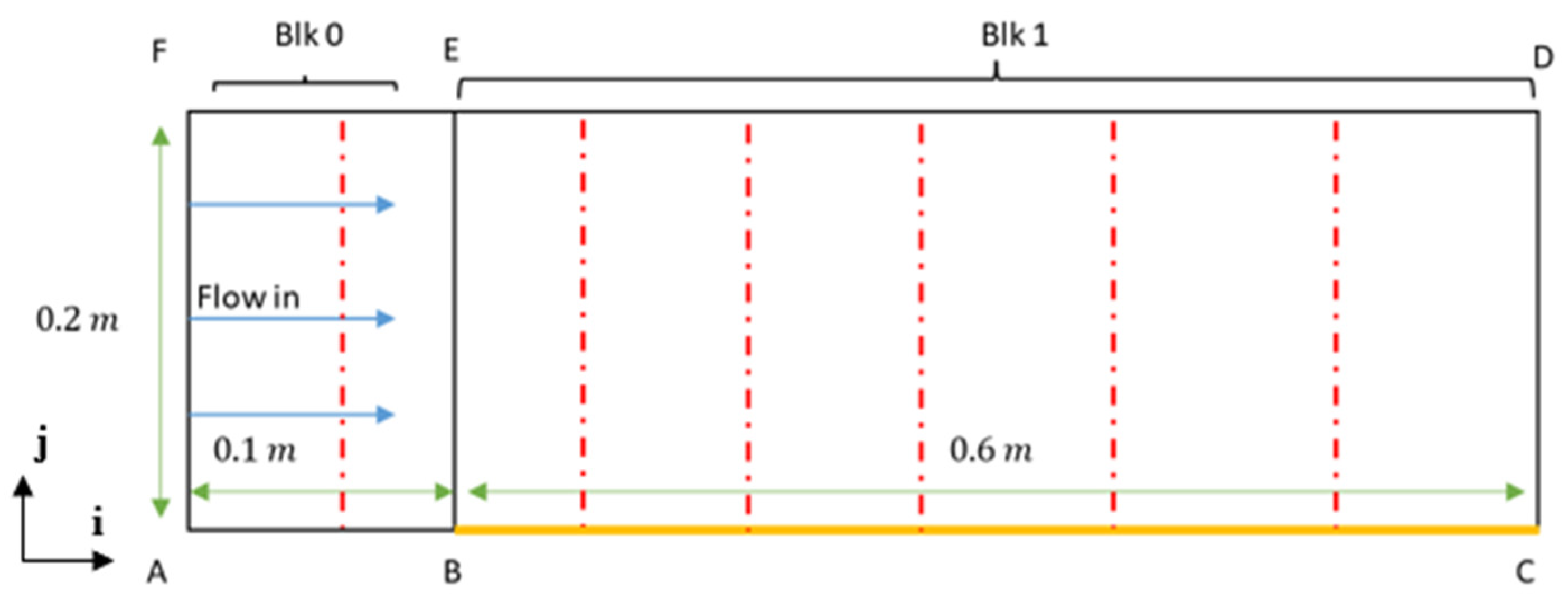
2.2. Eilmer and Numerical Plate Model

The SA-BCM model tested in this work is implemented in Eilmer [35], an open-source computational fluid dynamics code developed at the University of Queensland to support research in hypersonic and high-temperature gas dynamics. Eilmer is a fluid simulation program which solves the physical quantities and chemical reactions of high-speed gas flow. It is written in the D programming language and uses an embedded Lua interpreter for configuration and run-time customization. Eilmer contains a wide range of customizable options, including gas models, turbulence models, and flux calculators. In this research, both the existing SA model and a laminar flow condition are compared with the SA-BCM model. The transitional flow model has been built into Eilmer by the first author. As shown in Appendix A, SA-BCM is available in the public repository for broader use.

To assess the performance of SA-BCM under high-velocity flow conditions, a flat-plate model from He and Morgan’s experiments [33]—which were conducted in the T4 free-piston shock tunnel at the University of Queensland—is chosen for the test. The plate is 600 mm long and 300 mm wide with a $30°$ tapered edge. The CFD flow condition is initially aligned with one of their experimental conditions: s00 from

Table 1. Flow condition for the simulation [33].

Simulation Case	${\mathit{H}}_0$ $\left(\raisebox{1ex}{$\mathbf{M}\mathbf{J}$}\!\left/ \!\raisebox{-1ex}{$\mathbf{k}\mathbf{g}$}\right.\right)$	${\mathit{T}}_{\mathit{\infty }}$ $\left(\mathbf{K}\right)$	${\mathit{p}}_{\mathit{\infty }}$ $\left(\mathbf{k}\mathbf{P}\mathbf{a}\right)$	${\mathit{M}}_{\mathit{\infty }}$	${\mathit{U}}_{\mathit{\infty }}$ $\left(\raisebox{1ex}{$\mathbf{m}$}\!\left/ \!\raisebox{-1ex}{$\mathbf{s}$}\right.\right)$	$\mathit{R}{\mathit{e}}_{\mathit{u}}$ $\left(\times {10}^6\right)$	$\mathit{R}{\mathit{e}}_{\mathit{t}}$ $\left(\times {10}^6\right)$	Pr
s00	2.45	254	3.25	6.52	2100	4.99	1.28	0.719
s01	7.00	867	3.28	5.74	3360	1.25	0.65	0.694
s02	2.35	240	5.22	6.55	2060	10.30	1.74	0.723
s03	6.40	770	5.00	5.81	3150	2.60	1.03	0.688
s04	2.88	310	8.70	6.48	2200	9.56	1.63	0.705
s05	9.19	1257	9.60	5.47	3810	2.18	0.71	0.713
s06	3.17	347	18.30	6.30	2380	20.80	2.81	0.697
s07	10.10	1340	23.80	5.46	4050	4.30	1.33	0.717

[33]. After successful implementation and calibration, seven other flow conditions are also tested. Additionally, the freestream kinematic viscosity is set to ${\tilde{\nu }}_{farfield}=0.025{\nu }_{\infty }$, while the value is ${\tilde{\nu }}_{farfield}=5{\nu }_{\infty }$ in the original SA model. Since the physical experiment was performed in a free-piston shock tunnel [33], the freestream turbulence intensity, $T{u}_{\infty }$, is chosen to meet the same shock-tunnel condition. Two studies have performed similar experiments in the same type of shock tunnel, where the freestream flow is around Mach 6 [36,37]. Based on those reports, the $T{u}_{\infty }$ value is set to 0.4% here. However, the value is not fixed and can be adjusted further to correct the model through the research. The turbulent Schmidt number is left to its default value of 0.75, while the turbulent Prandtl number (Pr) is adjusted to the dry air at low-pressure conditions [38]. The Pr for each simulation case is also listed in Table 1.

An ideal air–gas model is applied for all the simulations, which does not consider the chemical reaction of the gas. To simplify the domain, only a 2D plate model is built (see Figure 1). The topology for the CFD grid consists of two blocks: blk0 is a blank block in front of the plate, and blk1 is the block that contains the plate, which is highlighted in yellow. The blank block is needed to simulate a stagnation point in the correct manner, although this does result in a minor increase in the computing resources required. The plate boundary BC is set to the fixed temperature of 300 K. Since the contact time between the gas and the plate is extremely short (in the order of milliseconds), it is assumed that no temperature change happens during the test. Flow comes in from the AF boundary and exits through the CD boundary. The height of the model is large enough to contain the entire shock from the stagnation to the end of the plate. As the shock is relatively weak in a flat-plate model, the grid structure is not adapted to the shock shape.

Viscous effects are turned on to evaluate the interaction between the flow boundary layer and the plate surface. The details of the s00 simulation configuration script are demonstrated in Appendix B. A series of files are generated after the simulation which collect the flow quantities along the BC boundary. The data from the final timestep, after the simulation has converged, is then compared to the experimental measurements to verify the transition model [33]. The location of transition region is be determined via heat transfer. The overall results of each simulation are visualized via ParaView software (ParaView 5.6; Kitware; USA).

2.3. Simulation Configuration

All the different flow cases use the same configuration with the same structured grid, except the grid convergence study. During the grid convergence study, various cell sizes for the simulation grid are evaluated. All the simulations are run on the same hardware, as detailed in

Table 2. Hardware information.

Hardware	Detail
CPU	AMD Ryzen 7 5800X
GPU	Nvidia GeForce RTX 3070Ti
Installed RAM	$\mathrm{USCorsair} \mathrm{LPX} \mathrm{DDR}4 2\times 16GB$
Installed Disk Space	$\mathrm{Samsung} \mathrm{PM}9\mathrm{A}1 512GBSSD$
System	Ubuntu 20.04 LTS

.

Two cluster functions are used in the model. One is a fixed Roberts function that clusters to the BE boundary, improving the accuracy of the solution near the stagnation point. The cfx0 is in the block 0, and the cfx0 is in the block 1.

cfx0 = RobertsFunction:new{end0 = false, end1 = true, beta = 1.1}

(16)

cfx1 = RobertsFunction:new{end0 = true, end1 = false, beta = 1.1}

(17)

The second cluster function is based on a geometric series and is applied along the AC boundary to resolve the boundary layer.

$$\mathrm{cfy}=\mathrm{GeometricFunction}:\mathrm{new}\{\mathrm{a}=0.001, \mathrm{r}=1.2, \mathrm{N}=N{j}_0\}$$

(18)

where ‘a’ defines the smallest cell size close to the surface that is the ratio of the height of the block. The growth rate of the cell size is defined by parameter ‘r’, while the N represents the quantities. The number of cells in different directions is represented by and $Nj$, while 0 and 1 mean the block number.

The final grid information is demonstrated in

Table 3. Grid information.

Cell Size (m)	$\mathit{N}{\mathit{i}}_0$	$\mathit{N}{\mathit{j}}_0$	$\mathit{N}{\mathit{i}}_1$	$\mathit{N}{\mathit{j}}_1$	a	r	Max CFL
0.002	50	100	300	100	0.0001	1.2	20

, and the special configuration of the Lua script of the plate model is shown in

Table 4. Details of the configuration in flat-plate Lua script.

Configuration Parameter	Value
config.dimensions	2
config.axisymmetric	false
config.viscous	true
config.report_invalid_cells	true
config.compute_loads	true
config.dt_loads	$1\times {10}^{-5}$
config.flux_calculator	ausmdv
config.max_time	$2\times \frac{l_{BC}}{U_{\infty }}$
config.max_step	$5\times {10}^5$
config.dt_init	$1\times {10}^{-8}$
config.cfl_schedule	$\left\{\right\{0.0, 0.5\}, \{5\times {10}^{-5}$, 20.0}}
config.dt_plot	config.max_time/10.0
For Turbulence Only
config.turbulence_model	“spalart_allmaras” or “spalart_allmaras_bcm”
config.turbulence_prandtl_number	0.89 (default)
config.turbulence_schmidt_number	0.75 (default)
config.freestream_turbulent_intensity	0.4%

. To increase the simulation speed, the message passing interface (MPI) parallel strategy is implemented. blk0 and blk1 are equally divided into two and six blocks, respectively, via Eilmer’s FBArray function. Thus, there are eight fluid blocks in total, which are calculated by eight separate processors in parallel. The time stepping scheme is set to the backward Euler method. A Courant–Friedrichs–Lewy (CFL) schedule is used, rather than a fixed CFL value. The maximum CFL value is set to twenty. As for the max simulation time, it is defined by the two times plate length, $l_{BC}$, divided by the freestream flow velocity, $U_{\infty }$. Thus, the time is enough for the flow to pass the plate. AUSMDV is the chosen flux calculator in this simulation, which is relatively economical. It should be noticed that Prandtl number is adapted to different flow conditions, while $T{u}_{\infty }$ is adjusted to 1.6% in model calibration step to match the experimental results.

2.4. Grid Convergence Study Plan

A grid convergence study is conducted before simulating different flow cases to assure the CFD is appropriately resolved. There are three interesting issues to investigate. The first one is the general cell size of the model. At this stage, there is no cluster function along the BE boundary, and only a fixed geometric function is implemented along the AC boundary, as defined in Equation (19). The general cell size is maintained as a square shape. Four different cell sizes are assessed at this stage, as shown in

Table 5. Test of general cell size.

Case No.	Cell Size (m)	$\mathit{N}{\mathit{i}}_0$	$\mathit{N}{\mathit{j}}_0$	$\mathit{N}{\mathit{i}}_1$	$\mathit{N}{\mathit{j}}_1$
1	0.004	25	40	150	40
2	0.0025	40	80	240	80
3	0.002	50	100	300	100
4	0.001	100	200	600	200

. The cell size is the length of the cell. The actual nodes in each direction are the cell number plus one.

cfy = RobertsFunction:new{end0 = true, end1 = false, beta = 1.02}

(19)

The second interesting issue is the parameters of the geometric cluster function, defined in Equation (18). The grid convergence study aims to find out how the parameters ‘a’ and ‘r’ in the geometric function impact the convergence. Under this test, the general cell size is set to 0.002 m. ‘a’ is tested from 0.01 to 0.00004, while ‘r’ is tested from 1.05 to 1.2.

Finally, a separate convergence study investigates the effect of the CFL schedule. Since different time-stepping schemes are sensitive to the CFL value, the maximum CFL value in the CFL schedule is assessed in the grid convergence section. To simplify the test process, only the maximum CFL value is adjusted in the schedule. The results of the convergence study are presented in the next section. After completing the convergence study, the SA-BCM model is applied to other flow conditions using the coarsest grid that properly resolves the required gradients.

3. Results

This section illustrates the results of the grid convergence study, as well as the SA-BCM model calibration and simulations of different flow cases. At first, the flat plate model is verified in a grid convergence study. Secondly, the freestream turbulence intensity is calibrated with the s00 flow case, the value of which is eventually set to 1.4%. Finally, the model with the new freestream turbulence intensity value is assessed with eight widely different hypersonic flow conditions. For ease of comparison, a new coordinate ‘x’ is introduced, which ignores the blank block and starts from the front point B to point C in Figure 1. All the simulations are conducted with the 2D flat-plate model. This research mainly focuses on the heat transfer in the boundary layer, which can directly reflect the transition start point.

3.1. Results of Grid Convergence Study

This section presents three approaches to grid convergence. The first is general cell size. The second is the geometric cluster function, and the final one is the max CFL value in the CFL schedule, which affects the time-accurate solutions. All the convergence studies are based on the flow condition of the s00 case in Table 1, and all the cases use $T{u}_{\infty }=4\%$. The reason for selecting the specific $T{u}_{\infty }$ is because the lower value of $T{u}_{\infty }$ in some grids cannot turn on the turbulent effect of the SA-BCM model.

The resulting heat transfer along the plate surfaces with different general cell size is plotted in Figure 2. However, there is no evident sign of convergence of adjusting this variable. Additionally, the rising cell quantities dramatically increase the running time of a script. When the general cell size is reduced to 0.001 m, the running time costs over one hour. Since the most interested area is the boundary layer, the geometric cluster function should play a more important role. When the cell size is smaller than 0.001 m, it is also found that the setting conflicts with the geometric cluster function and can cause geometry distortion.

Next, two parameters of geometric function are investigated, which are ‘a’ and ‘r’ in Equation (18). At first, variations of the cell ratio ‘a’ are assessed, while the growth rate, ‘r’, is set to 1.2. ‘a’ is reduced from 0.01 to 0.00004, Figure 3. The convergence is observed when ‘a’ reaches 0.0001. At this value, the laminar region and turbulent region highly converge. However, there is still minor gap in the transition region, as shown in red circle in Figure 3. When ‘a’ starts from 0.01 to 0.0001, the running time rises from 3 min to 90 min. Considering the finiteness of computing resources, a = 0.0001 is chosen as sufficient for this research. In addition to the SA-BCM model, the result of the SA model also shows convergence, as presented by Figure A1.

Normally, the growth rate is not as important as the cell ratio to the boundary layer. This research investigates it regardless. For convenience, ‘a’ is set to 0.001 at this stage. The growth rate, ‘r’, varies from 1.05 to 1.35. The result indicates no evident effect of convergence, and the heat transfer function fluctuates like a sine function in the transition region (Figure 4). Therefore, the growth rate retains 1.2 for the later simulation.

Initially, the maximum CFL value was set to 50. However, instabilities are observed within the heat transfer graph in this case. After the max CFL value is reduced to twenty, the heat transfer function becomes much more stable. To figure out whether this configuration affects convergence, the value is reduced further, and the results are demonstrated in Figure 5. The difference among them is extremely small. Thus, the max CFL value, 20, is enough for this research. As a result, the grid information presented in Table 3 is used for the subsequent studies.

3.2. SA-BCM Model Calibration

The flow condition s00 is applied, and the transition onset location is calibrated to He and Morgan’s paper [33] by adjusting the applied freestream turbulence intensity assumed by the code. The final grid structure is shown in Figure 6. The comparison of different $T{u}_{\infty }$ values in the SA-BCM model is indicated in Figure 7. The performance of SA-BCM model is compared to the laminar model and the original fully turbulent SA model. There is a clear indication that the SA-BCM model transforms from the laminar model to the SA turbulent model. The transition onset point is found by comparing the SA-BCM model to the laminar model at 1% difference. The reference transition onset point is $x_t=0$.256 m [33]. The deviation of each case is shown in

Table 6. Comparison of the results of SA-BCM model with experiment data.

$\mathit{T}{\mathit{u}}_{\mathit{\infty }}$	Transition Onset Point $x_t { }^1$	Error of $x_t$ to Reference	$q_{la}$ (J)	$q_{sb}$ (J)	$q_{sa}$at$x=0.5$(J)	$q_{sb}$at$x=0.5$(J)	Difference
4.0%	0.111	−56.69%	$8.08\times {10}^4$	$8.29\times {10}^4$	$1.52\times {10}^5$	$1.54\times {10}^5$	1.60%
2.5%	0.168	−34.26%	$6.53\times {10}^4$	$6.69\times {10}^4$	$1.52\times {10}^5$	$1.57\times {10}^5$	3.19%
2.0%	0.213	−16.92%	$5.80\times {10}^4$	$6.06\times {10}^4$	$1.52\times {10}^5$	$1.58\times {10}^5$	4.47%
1.7%	0.234	−8.45%	$5.53\times {10}^4$	$5.74\times {10}^4$	$1.52\times {10}^5$	$1.60\times {10}^5$	5.24%
1.6%	0.246	−4.04%	$5.40\times {10}^4$	$5.53\times {10}^4$	$1.52\times {10}^5$	$1.60\times {10}^5$	5.66%
1.5%	0.269	5.13%	$5.16\times {10}^4$	5.31 × 104	1.52 × 105	1.62 × 105	6.48%
0.4%	N/A	N/A	N/A	N/A	$1.52\times {10}^5$	$4.27\times {10}^5$	−71.84%

¹ The subscript t means transition onset point. The Laminar model and SA turbulent model are represented by la and sa. The notation sb means SA-BCM model.

. The total heat transfer q of each model at the transition point is also calculated. After that, the percentage difference between the SA model and the SA-BCM model in the fully turbulent region at $x=0.5 \mathrm{m}$ is compared as well. The result indicates that the SA-BCM model has the least error compared to the experiment result, as $T{u}_{\infty }=1.6\%$. This value is used to evaluate the model in different flow conditions. It should also be noted that $T{u}_{\infty }=0.4\%$ is too small to turn on the turbulence and the SA-BCM result is exactly same as the laminar model.

3.3. Simulation of Different Flow Conditions

The simulation results of eight flow cases are presented in this section. The performance of the SA-BCM model is compared to a laminar model and a fully turbulent SA model in each case, plotted in Figure 8. As calibrated in the previous section, the SA-BCM model switches from laminar flow to turbulent flow smoothly in the s00 case. The evidence of transition is also visible in the flow profiles (Figure A2, Figure A3, Figure A4, Figure A5, Figure A6, Figure A7, Figure A8 and Figure A9). However, the results of the SA-BCM model are the same as the laminar model in the s01 case, and it fails again in the s03 case. The turbulent effects seem to be underestimated in the s05 case. Besides these, the SA-BCM model seems to work well in the other flow conditions. This study also investigates the error between the transition onset point of the simulation result and the experimental results of each flow case from He and Morgan [33] (

Table 7. Transition onset locations under different flow cases.

Simulation Case	Reference $x_t$ [33] (m)	Simulation $x_t$ (m)	Error (%)
s00	0.256	0.245	−4.51
s01	0.520	N/A	N/A
s02	0.169	0.158	−6.27
s03	0.396	N/A	N/A
s04	0.171	0.132	−22.60
s05	0.326	0.508	56.12
s06	0.135	0.077	−43.07
s07	0.309	0.213	−31.17

). Additionally, the percentage error map against the flow Mach number is plotted in Figure 9. The y+ of the first cell of the flat plate in each case is demonstrated in

Table 8. y+ of the first cell over the flat plate in each case.

Simulation Case	y+ of Laminar Model	y+ of SA Model	y+ of SA-BCM Model
s00	6.64	6.65	6.64
s01	2.87	2.87	2.87
s02	8.44	8.50	8.44
s03	3.88	3.88	3.88
s04	9.04	9.17	9.04
s05	3.84	3.84	3.84
s06	11.42	12.48	11.42
s07	5.77	5.78	5.77

. The maximum dx values of all the flow cases and different flow models are the same, which are $3.35\times {10}^{-3}$ m. Similarly, the minimum dx is $5.84\times {10}^{-4}$ m for all the simulations. Since it is a 2D model, there is no z direction.

4. Discussion

4.1. About the Grid Convergence Study

The grid convergence study has investigated three factors that impact the grid accuracy, including the general cell size in the freestream, the geometric cluster function along the plate surface, and the max CFL value used for the backward Euler stepping scheme. The results show that it is the parameter ‘a’ of the geometric cluster function that impacts the boundary flow most significantly. The second most important factor is the max CFL value in the CFL schedule. As explained by this research, it seems the max CFL value lower than twenty makes the simulation converge neatly in time, as compared to larger values where noise is observed.

The general cell size in the freestream area may possess less impact on the boundary flow, compared to the cell size in the boundary area. Additionally, too small overall cell size can conflict with the geometric cluster function and result in geometry distortion. Thus, it is recommended that the general grid size should be defined with caution when the geometric function is used. Despite this, the grid convergence reveals that the transition length predicted by the SA-BCM model is highly sensitive to the grid size. Even though the laminar region and turbulent region converges to a certain value, the transition region keeps fluctuating around some points (Figure 3 and Figure 4).

Another concern is the y+ value in this study. The overall y+ value is quite high. When y+ is greater than five, the turbulent onset point may take place early [39]. Since s01, s03 and s05 cases possess relatively low y+, the transition of these three cases may be turned on slower than the others with higher y+. However, the grid convergence study indicates that further reduction in cell size along the boundary layer does not have much effect on the turbulent onset location when ‘a’ is less than 0.0002. On the contrary, this action can significantly increase the simulation time. While a = 0.00004, the simulation costs more than nine hours to run. Thus, the large y+ value should not account for the inaccuracy of this model. For the ease of simulating and adjusting codes at the development stage, configures with short running time are still preferred.

4.2. Performance of SA-BCM Model in Hypersonic Flow

The prediction of the transition onset location in the s00 flow condition shows good agreement with the shock tunnel experiment [33] after the modification of turbulence intensity in Table 6. When $T{u}_{\infty }$ is set to 1.6%, the most accurate transition onset location is obtained. The obtained transition onset location is $x_t=0$.246 m, compared to $x_t$ $=0$.256 m in the experiment [33]. Figure 8a indicates that the SA-BCM model perfectly fits the laminar model before the transition and matches the SA turbulence model after transition. The laminar flow gradually changes into turbulent flow in the transition region. This evidence proves the ability of the SA-BCM model to potentially predict the hypersonic transitional flow, after appropriate calibration. The transition is also observed in the profiles of physical quantities of the flow. The laminar model has no turbulence, while the SA model generates turbulent viscosity at the leading edge of the plate. Only the SA-BCM model shows a transition from laminar flow to turbulent flow. This phenomenon is distinctive in ${\mu }_t$ and $\widehat{\nu }$ profiles. As in ${\mu }_t$ profiles, there is no turbulence and the ${\mu }_t$ is completely missing in the boundary region of the laminar model, while ${\mu }_t$ starts from the stagnation point in the SA model. In the SA-BCM model, there is a delay before the beginning of the rise in ${\mu }_t$. This delay indicates the flow is still laminar in that region.

However, the calibrated turbulence intensity disagrees with the experimental measurements of the T4 free-piston shock tunnel [36]. At a similar flow condition to s00 in a similar shock tunnel, $T{u}_{\infty }$ is around 0.4%, rather than 1.6%. One likely reason for this is that the measurement of turbulence intensity is not accurate. Another reason could be that the constant of ${\Re }_{\theta c}$ function in the SA-BCM model is not designed for hypersonic flow conditions. Moreover, this research finds that a higher $T{u}_{\infty }$ value may increase the running time of the simulations dramatically.

The performance of SA-BCM in different flow conditions is also unsatisfactory. The model fails to predict the transition in the s01 and s03 cases. One probable reason for this may be that $T{u}_{\infty }$ is too small to turn on the turbulence in the s01 and s03 cases. This hypothesis is supported by the s05 and s06 cases. In the s05 case, transition is observed near the end of the plate, while the transition occurs too early in the s06 case. Thus, the accuracy of the SA-BCM model is significantly affected by $T{u}_{\infty }$ in hypersonic flow. Additionally, the SA-BCM model can be accurate in different flow cases if the $T{u}_{\infty }$ is calibrated with different flow conditions. In this case, the flow model should be precise and able to adopt appropriate $T{u}_{\infty }$ in certain conditions. However, this may require a table of $T{u}_{\infty }$ to be built in the program and raise the programming complexity.

According to Table 7, it seems that the SA-BCM model with calibrated $T{u}_{\infty }$ from one flow condition is not accurate in other cases. As shown in Figure 9, the error in the SA-BCM model is unlikely to have a linear relationship with the Mach number. It may relate to the specific enthalpy and internal energy of the flow. This drawback introduces complexities into the use of the SA-BCM model, as it always requires calibrating in different flow conditions.

4.3. $T{u}_{\infty }$ and ${\gamma }_{BC}$ in SA-BCM Model

The constant parameters in the SA-BCM model could lead the simulation to predict wrong results at high-velocity flow. Thus far, all the results indicate the error within the SA-BCM model relating to the $T{u}_{\infty }$ value. It seems the SA-BCM model gives invalid results due to the wrong $T{u}_{\infty }$. However, the similar hypersonic flow condition where $T{u}_{\infty }$ equals 0.4% is also used in two papers. One is in simulation with the $\gamma -R{e}_{\theta t}$ model and the $k-\omega -\gamma$ model [37]. Another one is tested with a one-equation γ model [40]. The second case defines a flat plate with an adiabatic condition, rather than fixed temperature. All these models work well with $T{u}_{\infty }$ = 0.4%. As a result, the freestream turbulence intensity value is not the source of the misconduct of the SA-BCM model. Other parameters inside the ${\gamma }_{BC}$ term may be relevant to the problem.

A deep look into the SA-BCM model shows that the constants are calibrated by the low-velocity test, and the ${\chi }_2$ inside the ${\gamma }_{BC}$ is calibrated from Schubauer and Klebanoff’s flat-plate test [34]. The highest flow speed in those wind tunnel experiments was 42.7 m/s, which is extremely low compared to the simulation cases in this research. According to Table 1 [33], the lowest flow velocity is 2100 m/s in the s00 case. Thus, those constants can cause trouble in high-enthalpy and high-velocity flow. The effort of calibrating $T{u}_{\infty }$ is the compensation for the inaccurate constants within the SA-BCM model under high-velocity flow. If the constant inside the ${\gamma }_{BC}$ model can be recalibrated with a new physical experimental result from supersonic or hypersonic flow tests, it may be possible to apply SA-BCM to general high-velocity flow problems.

4.4. Comparison with Modified $\gamma -R{e}_{\theta t}$ Model

The original $\gamma -R{e}_{\theta t}$ model, proposed by Menter et al. [39], is a two-equation model based on the LCTM concept. The model is widely adopted and has a few modified versions which are adapted to hypersonic flow problems [2,41,42,43]. After a few years, Menter et al. [44] announced a simplified one-equation γ model. The new model eliminates the lack of Galilean invariance and removes the transitional Reynold’s number $R{e}_{\theta t}$ in the transport equation. In 2020, an improved one-equation $\gamma$ model is proposed by Liu et al. [40]. Compared to the Menter’s model [44], the key difference is that $R{e}_{\theta }$ and $\gamma$ are modified to simulate high-speed transitional flow. The new $\gamma$ considers the physical information of the flow. A new feature is the introduction of the Fr term based on Hao’s research [45]. This replaced the $R{e}_{v,max}$ term in the original equation, which is not compatible with hypersonic boundary conditions [2]. Another important update is to add the $f\left(T{u}_{\infty }\right)$ term, which is inspired by Yang et al. [46].

The improved one-equation γ model has been tested by Liu et al. [40] in a supersonic flat-plate case [47], a hypersonic flat-plate case [30], a slender-cone case [48], a X-51A forebody case [49], and a hypersonic inflatable aerodynamic decelerator case [50,51]. All the results indicate that the improved model has significantly increasing accuracy. Although the original model has problems with predicting the skin fraction along an adiabatic flat plate, the modified version can accurately predict the transition starting point and flow quantity [40]. This new modified model may have an advantage over the SA-BCM model based on accuracy. However, the SA-BCM model is not fully calibrated for hypersonic flow and the potential for this model is still uncertain. In practical programming, the software may need an additional equation to find the turbulent frequency, $\omega$. Another transport equation is also needed to calculate the turbulent kinetic energy, k. As a result, this two-equation model is expected to cost much more in terms of computing resources than one-equation SA-BCM model.

5. Conclusions

This paper presents research into the performance of the SA-BCM turbulent transition model for high-velocity flow. The model is tested in a flat-plate CFD simulation with eight different flow conditions [33]. The SA-BCM model has the potential to predict the transition region in hypersonic conditions with calibrated $T{u}_{\infty }$. However, there are two evident shortcomings. Primarily, the heat transfer in the transition region is extremely sensitive to the local grid size. Even though the laminar region and the turbulent region of the SA-BCM model converged in our grid convergence study, the transition region may still be unstable. Secondly, the accuracy of the SA-BCM model relies on the precise tuning of $T{u}_{\infty }$. To increase the accuracy, different flow conditions may require a corresponding $T{u}_{\infty }$ value. As demonstrated in this research, a single $T{u}_{\infty }$ calibrated from the s00 case does not give accurate flow solutions in other flow conditions. As a result, this drawback restricts the application of the model.

It is the constant in ${\gamma }_{BC}$ term that should account for the shortcomings, rather than $T{u}_{\infty }$. The original ${\gamma }_{BC}$ term is calibrated with low-velocity flow data, which are unlikely to predict high-velocity flow in the correct manner. Adjusting $T{u}_{\infty }$ only compensates for some model constants, which cannot solve the intrinsic problems within the SA-BCM model. Although the application of this model is restricted by the $T{u}_{\infty }$ and ${\gamma }_{BC}$ term, the SA-BCM is still accurate to use after the $T{u}_{\infty }$ has been calibrated. As a one-equation model, it is also fast to run and remains attractive to modern CFD. In conclusion, the performance of the SA-BCM model in hypersonic flow is summarized as follows:

• Possesses fast running speed;
• Has potential for industrial applications;
• Can partially solve hypersonic transitional flow;
• Requires calibration of $T{u}_{\infty }$ for complex flow conditions;
• Requires awareness that the transition region is sensitive to the grid;
• Needs recalibration of the model constants to solve intrinsic inaccuracy.

There are two recommendations for future research on this topic. One is to re-calibrate the ${\gamma }_{BC}$ term and make it suitable for supersonic and hypersonic flows. This may require extra effort in physical experiments. Another is to replace the ${\gamma }_{BC}$ term and combine the SA-BCM model with other transitional flow models. A practical way to do this may be to replace the ${\gamma }_{BC}$ term with the intermittency factor from the modified one-equation γ model [40]. However, this may cause other issues, as the one-equation γ model needs turbulent kinetic energy, k, and turbulent frequency, ω. This would, however, require hybridization with the k and ω calculated from the k − ω equations [15], which would somewhat increase the running time and would require new model development.

References

1. Schneider, S.P. Laminar-Turbulent Transition on Reentry Capsules and Planetary Probes. J. Spacecr. Rocket. 2006, 43, 1153–1173. [Google Scholar] [CrossRef]
2. Frauholz, S.; Reinartz, B.U.; Müller, S.; Behr, M. Transition Prediction for Scramjets Using γ-Reθt Model Coupled to Two Turbulence Models. J. Propuls. Power 2015, 31, 1404–1422. [Google Scholar] [CrossRef]
3. Sommer, S.C.; Compton, D.L.; Short, B.J.; Ames Research Center. Free-Flight Measurements of Static and Dynamic Stability of Models of the Project Mercury Re-Entry Capsule at Mach Numbers 3 and 9.5; National Aeronautics and Space Administration: Washington DC, USA, 1960.
4. Michna, J.; Rogowski, K.; Bangga, G.; Hansen, M.O.L. Accuracy of the Gamma Re-Theta Transition Model for Simulating the DU-91-W2-250 Airfoil at High Reynolds Numbers. Energies 2021, 14, 8224. [Google Scholar] [CrossRef]
5. Schneider, S.P. Effects of High-Speed Tunnel Noise on Laminar-Turbulent Transition. J. Spacecr. Rocket. 2001, 38, 323–333. [Google Scholar] [CrossRef]
6. Schneider, S.P. Hypersonic Laminar–Turbulent Transition on Circular Cones and Scramjet Forebodies. Prog. Aerosp. Sci. 2004, 40, 1–50. [Google Scholar] [CrossRef]
7. Saric, W.S. Görtler Vortices. Annu. Rev. Fluid Mech. 1994, 26, 379–409. [Google Scholar] [CrossRef]
8. Mack, L.M. Boundary-Layer Linear Stability Theory; California Inst of Tech Pasadena Jet Propulsion Lab: La Cañada Flintridge, CA, USA, 1984. [Google Scholar]
9. Reed, H.L.; Lin, R.-S. Stability of Three-Dimensional Boundary Layers; SAE: Warrendale, PA, USA, 1987. [Google Scholar]
10. Kundu, A.; Thangadurai, M.; Biswas, G. Investigation on Shear Layer Instabilities and Generation of Vortices during Shock Wave and Boundary Layer Interaction. Comput. Fluids 2021, 224, 104966. [Google Scholar] [CrossRef]
11. Beckwith, I.E.; Miller, C.G. Aerothermodynamics and Transition in High-Speed Wind Tunnels at NASA Langley. Annu. Rev. Fluid Mech. 1990, 22, 419–439. [Google Scholar] [CrossRef]
12. Spalart, P.; Allmaras, S. A One-Equation Turbulence Model for Aerodynamic Flows. In Proceedings of the 30th Aerospace Sciences Meeting and Exhibit, Reno, NV, USA, 6–9 January 1992; American Institute of Aeronautics and Astronautics: Reston, VA, USA, 1992. [Google Scholar]
13. Bradshaw, P.; Ferriss, D.H.; Atwell, N.P. Calculation of Boundary-Layer Development Using the Turbulent Energy Equation. J. Fluid Mech. 1967, 28, 593–616. [Google Scholar] [CrossRef]
14. Jones, W.P.; Launder, B.E. The Prediction of Laminarization with a Two-Equation Model of Turbulence. Int. J. Heat Mass Transf. 1972, 15, 301–314. [Google Scholar] [CrossRef]
15. Wilcox, D.C. Formulation of the K-w Turbulence Model Revisited. AIAA J. 2008, 46, 2823–2838. [Google Scholar] [CrossRef]
16. Menter, F.R. Two-Equation Eddy-Viscosity Turbulence Models for Engineering Applications. AIAA J. 1994, 32, 1598–1605. [Google Scholar] [CrossRef]
17. Launder, B.E.; Reece, G.J.; Rodi, W. Progress in the Development of a Reynolds-Stress Turbulence Closure. J. Fluid Mech. 1975, 68, 537–566. [Google Scholar] [CrossRef]
18. Crivellini, A.; D’Alessandro, V. Spalart–Allmaras Model Apparent Transition and RANS Simulations of Laminar Separation Bubbles on Airfoils. Int. J. Heat Fluid Flow 2014, 47, 70–83. [Google Scholar] [CrossRef]
19. Sai, V.A.; Lutfy, F.M. Analysis of the Baldwin-Barth and Spalart-Allmaras One-Equation Turbulence Model. AIAA J. 1995, 33, 1971–1974. [Google Scholar] [CrossRef]
20. Cebeci, T. Analysis of Turbulent Flows with Computer Programs; Elsevier Science & Technology: Oxford, UK, 2013; ISBN 978-0-08-098335-6. [Google Scholar]
21. Karvinen, A.; Ahlstedt, H. Comparison of Turbulence Models in Case of Three-Dimensional Diffuser. In Proceedings of the Open Source CFD International Conference 2008, Berlin, Germany, 4–5 December 2008. [Google Scholar]
22. Miroshnichenko, I.; Sheremet, M. Comparative Study of Standard k –ε and k –ω Turbulence Models by Giving an Analysis of Turbulent Natural Convection in an Enclosure. EPJ Web Conf. 2015, 82, 01057. [Google Scholar] [CrossRef]
23. Rodi, W. DNS and LES of Some Engineering Flows. Fluid Dyn. Res. 2006, 38, 145–173. [Google Scholar] [CrossRef]
24. Yang, X.I.A.; Griffin, K.P. Grid-Point and Time-Step Requirements for Direct Numerical Simulation and Large-Eddy Simulation. Phys. Fluids 2021, 33, 015108. [Google Scholar] [CrossRef]
25. Kendall, J. Experiments on Boundary-Layer Receptivity to Freestream Turbulence. In Proceedings of the 36th AIAA Aerospace Sciences Meeting and Exhibit, Reno, NV, USA, 12–15 January 1998; American Institute of Aeronautics and Astronautics: Reston, VA, USA, 1998. [Google Scholar]
26. Klebanoff, P.S.; Tidstrom, K.D.; Sargent, L.M. The Three-Dimensional Nature of Boundary-Layer Instability. J. Fluid Mech. 1962, 12, 1–34. [Google Scholar] [CrossRef]
27. Zhao, Y.; Lei, C.; Patterson, J.C. The K-Type and H-Type Transitions of Natural Convection Boundary Layers. J. Fluid Mech. 2017, 824, 352–387. [Google Scholar] [CrossRef]
28. Sayadi, T.; Hamman, C.W.; Moin, P. Direct Numerical Simulation of H-Type and K-Type Transition to Turbulence; Center for Turbulence Research Annual Research Briefs; NASA Ames: Mountain View, CA, USA, 2011; pp. 109–121.
29. Xu, J.; Liu, J.; Mughal, S.; Yu, P.; Bai, J. Secondary Instability of Mack Mode Disturbances in Hypersonic Boundary Layers over Micro-Porous Surface. Phys. Fluids 2020, 32, 044105. [Google Scholar] [CrossRef]
30. Mee, D.J. Boundary-Layer Transition Measurements in Hypervelocity Flows in a Shock Tunnel. AIAA J. 2002, 40, 1542–1548. [Google Scholar] [CrossRef]
31. Anderson, J.D. Hypersonic and High-Temperature Gas Dynamics, 3rd ed.; American Institute of Aeronautics & Astronautics: Reston, VA, USA, 2019; ISBN 978-1-62410-645-3. [Google Scholar]
32. Cakmakcioglu, S.C.; Bas, O.; Mura, R.; Kaynak, U. A Revised One-Equation Transitional Model for External Aerodynamics. In Proceedings of the AIAA AVIATION 2020 FORUM, Virtual Event, 15–19 June 2020; American Institute of Aeronautics and Astronautics: Reston, VA, USA, 2020. [Google Scholar]
33. He, Y.; Morgan, R.G. Transition of Compressible High Enthalpy Boundary Layer Flow over a Flat Plate. Aeronaut. J. 1994, 98, 25–34. [Google Scholar] [CrossRef]
34. Schubauer, G.B.; Klebanoff, P.S. Contributions on the Mechanics of Boundary-Layer Transition; National Advisory Committee For Aeronautics; NACA: Washington, DC, USA, 1955.
35. Gibbons, N.N.; Damm, K.A.; Jacobs, P.A.; Gollan, R.J. Eilmer: An Open-Source Multi-Physics Hypersonic Flow Solver. arXiv 2022, arXiv:2206.01386. [Google Scholar]
36. Papp, J.L.; Dash, S.M. Rapid Engineering Approach to Modeling Hypersonic Laminar-To-Turbulent Transitional Flows. J. Spacecr. Rocket. 2005, 42, 467–475. [Google Scholar] [CrossRef]
37. Zhao, Y.; Yan, C.; Liu, H.; Zhang, K. Uncertainty and Sensitivity Analysis of Flow Parameters for Transition Models on Hypersonic Flows. Int. J. Heat Mass Transf. 2019, 135, 1286–1299. [Google Scholar] [CrossRef]
38. Rogers, G.F.C.; Mayhew, Y.R. Thermodynamic and Transport Properties of Fluids: SI Units, 5th ed.; reprinted; SI units; Blackwell: Oxford, UK, 2003; ISBN 978-0-631-19703-4. [Google Scholar]
39. Menter, F.R.; Langtry, R.B.; Likki, S.R.; Suzen, Y.B.; Huang, P.G.; Völker, S. A Correlation-Based Transition Model Using Local Variables—Part I: Model Formulation. J. Turbomach. 2006, 128, 413. [Google Scholar] [CrossRef]
40. Liu, Z.; Yan, C.; Cai, F.; Yu, J.; Lu, Y. An Improved Local Correlation-Based Intermittency Transition Model Appropriate for High-Speed Flow Heat Transfer. Aerosp. Sci. Technol. 2020, 106, 106122. [Google Scholar] [CrossRef]
41. Krause, M.; Behr, M.; Ballmann, J. Modeling of Transition Effects in Hypersonic Intake Flows Using a Correlation-Based Intermittency Model. In Proceedings of the 15th AIAA International Space Planes and Hypersonic Systems and Technologies Conference, Dayton, OH, USA, 28 April–1 May 2008; American Institute of Aeronautics and Astronautics: Reston, VA, USA, 2008. [Google Scholar]
42. You, Y.; Luedeke, H.; Eggers, T.; Hannemann, K. Application of the Y-Reot Transition Model in High Speed Flows. In Proceedings of the 18th AIAA/3AF International Space Planes and Hypersonic Systems and Technologies Conference, Tours, France, 24–28 September 2012; American Institute of Aeronautics and Astronautics: Reston, VA, USA, 2012. [Google Scholar]
43. de Rosa, D.; Catalano, P. RANS Simulations of Transitional Flow by γ Model. Int. J. Comput. Fluid Dyn. 2019, 33, 407–420. [Google Scholar] [CrossRef]
44. Menter, F.R.; Smirnov, P.E.; Liu, T.; Avancha, R. A One-Equation Local Correlation-Based Transition Model. Flow Turbul. Combust. 2015, 95, 583–619. [Google Scholar] [CrossRef]
45. Hao, Z.; Yan, C.; Qin, Y.; Zhou, L. Improved γ-Reθt Model for Heat Transfer Prediction of Hypersonic Boundary Layer Transition. Int. J. Heat Mass Transf. 2017, 107, 329–338. [Google Scholar] [CrossRef]
46. Yang, M.; Xiao, Z. Distributed Roughness Induced Transition on Wind-Turbine Airfoils Simulated by Four-Equation k-ω-γ-Ar Transition Model. Renew. Energy 2019, 135, 1166–1177. [Google Scholar] [CrossRef]
47. Pirozzoli, S.; Grasso, F.; Gatski, T.B. Direct Numerical Simulation and Analysis of a Spatially Evolving Supersonic Turbulent Boundary Layer at M=2.25. Phys. Fluids 2004, 16, 530–545. [Google Scholar] [CrossRef]
48. Horvath, T.; Berry, S.; Hollis, B.; Singer, B.; Chang, C.-L. Boundary Layer Transition on Slender Cones in Conventional and Low Disturbance Mach 6 Wind Tunnels. In Proceedings of the 32nd AIAA Fluid Dynamics Conference and Exhibit, St. Louis, MO, USA, 24–26 June 2002; American Institute of Aeronautics and Astronautics: Reston, VA, USA, 2012. [Google Scholar]
49. Borg, M.; Schneider, S. Effect of Freestream Noise on Instability and Transition for the X-51A Lee Side. In Proceedings of the 47th AIAA Aerospace Sciences Meeting including The New Horizons Forum and Aerospace Exposition, Orlando, FL, USA, 5–8 January 2009; American Institute of Aeronautics and Astronautics: Reston, VA, USA, 2009. [Google Scholar]
50. Hollis, B.R.; Hollingsworth, K.E. Experimental Study of Hypersonic Inflatable Aerodynamic Decelerator (HIAD) Aeroshell with Axisymmetric Surface Deflection Patterns; NASA: Washington, DC, USA, 2017.
51. Hollis, B.R. Surface Heating and Boundary-Layer Transition on a Hypersonic Inflatable Aerodynamic Decelerator. J. Spacecr. Rocket. 2018, 55, 856–876. [Google Scholar] [CrossRef]
Figure 1. Demonstration of the flat-plate model.
Mathematics 10 03431 g001
Figure 2. Grid convergence study of general cell size.
Mathematics 10 03431 g002
Figure 3. Grid convergence study of cell ratio ‘a’.
Mathematics 10 03431 g003
Figure 4. Grid convergence study of growth ratio ‘r’.
Mathematics 10 03431 g004
Figure 5. Grid convergence study of max CFL value.
Mathematics 10 03431 g005
Figure 6. Grid of the flat plate.
Mathematics 10 03431 g006
Figure 7. Calibration of freestream turbulence intensity.
Mathematics 10 03431 g007
Figure 8. Flow model comparison: (a) s00 case; (b) s01 case; (c) s02 case; (d) s03 case; (e) s04 case; (f) s05 case; (g) s06 case; (h) s07 case.
Mathematics 10 03431 g008aMathematics 10 03431 g008b
Figure 9. Error of different flow cases against Mach number.
Mathematics 10 03431 g009