The Dimensionality Reduction of Crank–Nicolson Mixed Finite Element Solution Coefficient Vectors for the Unsteady Stokes Equation

Abstract

By means of a proper orthogonal decomposition (POD) to cut down the dimensionality of unknown finite element (FE) solution coefficient vectors in the Crank–Nicolson (CN) mixed FE (CNMFE) method for two-dimensional (2D) unsteady Stokes equations in regard to vorticity stream functions, a reduced dimension recursive-CNMFE (RDR-CNMFE) method is constructed. In this case, the RDR-CNMFE method has the same FE basis functions and accuracy as the CNMFE method. The existence, stability, and errors of RDR-CNMFE solutions are analyzed by matrix analyzing, resulting in very simple theory analysis. Some numerical tries are used to check on the validity of the RDR-CNMFE method. The RDR-CNMFE method has second-order time accuracy and few unknowns so as to be able to shorten CPU runtime and retard the error cumulation in simulation calculating process, and improve real-time calculating accuracy.

1. Introduction

Let $\mathsf{\Omega }\subset {\mathbb{R}}^2$ be a bounded connected domain, and consider the following two-dimensional (2D) unsteady Stokes Equation (see [1,2]).

Problem 1.

Find ${(u,v)}^T$ and p such that

$$\begin{array}{ccc}\hfill & & {\displaystyle {\partial }_{t}u-\nu \Delta u+{\partial }_{x}p=g_1,(t,x,y)\in (0,t_e)\times \mathsf{\Omega },}\hfill \end{array}$$

(1)

$$\begin{array}{ccc}& & {\displaystyle {\partial }_{t}v-\nu \Delta v+{\partial }_{y}p=g_2,(t,x,y)\in (0,t_e)\times \mathsf{\Omega },}\hfill \end{array}$$

(2)

$$\begin{array}{ccc}\hfill & & {\displaystyle {\partial }_{x}u+{\partial }_{y}v=0,(t,x,y)\in (0,t_e)\times \mathsf{\Omega },}\hfill \end{array}$$

(3)

$$\begin{array}{ccc}\hfill & & {\displaystyle u(t,x,y)={\phi }_u(t,x,y),(t,x,y)\in (0,t_e]\times \partial \mathsf{\Omega },}\hfill \end{array}$$

(4)

$$\begin{array}{ccc}\hfill & & {\displaystyle v(t,x,y)={\phi }_v(t,x,y),(t,x,y)\in (0,t_e]\times \partial \mathsf{\Omega },}\hfill \end{array}$$

(5)

$$\begin{array}{ccc}& & {\displaystyle u(0,x,y)=u^0(x,y),v(0,x,y)=v^0(x,y),(x,y)\in \mathsf{\Omega },}\hfill \end{array}$$

(6)

wherein ${(u,v)}^T$ is the fluid velocity vector; p is the fluid pressure; $t_e$ is the final time; $Re$ is the Reynolds number; ${\partial }_z=\partial /\partial z$$(z=t,x,y)$, $\Delta u={\partial }^{2}u/\partial x^2+{\partial }^{2}u/\partial y^2$, $\Delta v={\partial }^{2}v/\partial x^2+{\partial }^{2}v/\partial y^2$, $\nu =1/Re$; and $(g_1(t,x,y),g_2(t,$${x,y\left)\right)}^T$, ${(u^0(x,y),v^0(x,y))}^T$, and $({\phi }_u(t,x,y),{\phi }_v(t,$${x,y\left)\right)}^T$ are the known vectors for the body force, boundary value, and initial value, respectively.

The unsteady Stokes equation is one of the most important fluid dynamic equations and has been used to simulate many natural phenomena (see, e.g., [1,2,3,4,5,6,7]). However, when the geometrical shape of computational domain is irregular, or the known vectors of body force and boundary initial and values are complex, it has no analytical solution, so one has to rely on numerical solutions.

The Crank–Nicolson (CN) mixed finite element (FE) (MFE) (CNMFE) method for the 2D unsteady Stokes equation about vorticity-stream functions has second-order time accuracy, unconditional stability, and unconditional convergence, so it is one of the most popular numerical methods. However, the CNMFE method, like other numerical methods, involves a large number of unknowns, such that its calculation load is very heavy, and rounding errors could be quickly accumulated in an actual numerical computation. Hence, the main task herein is to cut down the unknowns in the CNMFE method so as to shorten CPU runtime, retard the rounded error amassing, alleviate the calculated burden, and enhance high calculation efficiency.

Lots of examples (see [8,9,10,11,12,13,14,15,16]) have shown that the proper orthogonal decomposition (POD) method is one of the most effective approaches to be able to lessen the unknowns in the numerical methods. Therefore, we herein employ the POD method to reduce the unknowns of CNMFE method by only lowering the dimensionality of unknown CNMFE solution coefficient vectors for unsteady Stokes equations so as to construct the reduced dimension recursive-CNMFE (RDR-CNMFE) method. In the case, the RDR-CNMFE method has the same FE basis functions and accuracy as the CNMFE method; moreover, it has only a few unknowns.

Although the reduced-dimension methods of the unknown FE solution coefficient vectors for the hyperbolic and parabolic equations, the Sobolev equation, and the Rosenau equation were, respectively, constructed in [17,18,19,20], the unsteady Stokes equation is more complicated than the four type of equations in [17,18,19,20], since it not only contains the fluid velocity vector, but also includes the pressure, so that both the construction for the RDR-CNMFE method and the theoretical analysis for the existence, stability, and convergence for the RDR-CNMFE solutions would face more difficulties and require more techniques than those in [17,18,19,20]; but the Stokes equation has very important applications (see, e.g., [1,2,3,4,5,6,7]). Thus, it is worthy to study the RDR-CNMFE method for the unsteady Stokes equation.

To this end, we first construct the unconditionally stable and unconditionally convergent CNMFE method with second-order time accuracy for the 2D unsteady Stokes equation about the vorticity-stream functions and analyze the existence, stability, and errors of the CNMFE solutions in Section 2. Next, in Section 3, we use the POD method to construct the POD basis vectors and RDR-CNMFE model, and adopt the matrix analysis to analyze the existence, stability, and erorrs for the RDR-CNMFE solutions. Then, we employ some numerical tests to exhibit the superiority of the RDR-CNMFE method and verify that the numerical calculation results are in accordance with the theoretical results in Section 4. Finally, we summarize main conclusions in Section 5.

2. The CNMFE Method for the Unsteady Stokes Equation

The Sobolev spaces and norms used herein are standard. For convenience, we assume that $\mathbb{V}=H_0^1\left(\mathsf{\Omega }\right)$, and for the sake of discussion, but without losing generality, we suppose that ${({\phi }_u(t,x,y),{\phi }_v(t,x,y))}^T=\mathbf{0}$ in the follow-up theoretical analysis.

Owing to the boundedness and connectedness of the domain $\mathsf{\Omega }$, the equation ${\partial }_{x}u+{\partial }_{y}v=0$ exists as a unique stream function $\psi$ such that $u={\partial }_y\psi$ and $v=-{\partial }_x\psi$. Further, there exists a vorticity function $\varpi$ such that $\varpi ={\partial }_{x}v-{\partial }_{y}u=-\Delta \psi$. Thus, Problem 1 can be turned into the following vorticity–stream forms:

$$\begin{array}{ccc}\hfill & & \left\{\begin{array}{c}{\displaystyle -▵\psi =\varpi ,(t,x,y)\in (0,t_e)\times \mathsf{\Omega },}\hfill \\ {\displaystyle \psi =0,(t,x,y)\in [0,t_e]\times \partial \mathsf{\Omega },}\hfill \end{array}\right.\hfill \end{array}$$

(7)

$$\begin{array}{ccc}\hfill & & \left\{\begin{array}{c}{\displaystyle {\partial }_t\varpi -\nu ▵\varpi =f={\partial }_x{g}_2-{\partial }_y{g}_1,(t,x,y)\in (0,t_e)\times \mathsf{\Omega },}\hfill \\ {\displaystyle \varpi =0,(t,x,y)\in [0,t_e]\times \partial \mathsf{\Omega },}\hfill \\ {\displaystyle \varpi ={\varpi }^0={\partial }_x{v}^0-{\partial }_y{u}^0,(x,y)\in \mathsf{\Omega }.}\hfill \end{array}\right.\hfill \end{array}$$

(8)

To construct the CNMFE method with second-order time accuracy, it is first necessary to discretize the first derivative of time in (8) by the CN method. Let $N>0$ denote the integer, let $\Delta t=t_e/N$ denote the time step, and let ${\varpi }^n(x,y)$ and ${\psi }^n(x,y)$ be, respectively, the approximations of $\varpi (t,x,y)$ and $\psi (x,y,t)$ at $t_n=n\Delta t$. Thus, a time semi-discretized format with second-order time accuracy can be constructed as follows.

Problem 2.

Find $({\varpi }^n,{\psi }^n)\in V\times V$$(1⩽n⩽N)$ such that

$$\begin{array}{ccc}\hfill & & {\displaystyle a({\psi }^{n-1},\chi )=({\varpi }^{n-1},\chi ),\forall \chi \in V,1⩽n⩽N+1;}\hfill \\ & & {\displaystyle ({\varpi }^n,\chi )+\frac{\nu \Delta t}{2}a({\varpi }^n+{\varpi }^{n-1},\chi )}\hfill \end{array}$$

(9)

$$\begin{array}{ccc}\hfill & & {\displaystyle =({\varpi }^{n-1},\chi )+\Delta t(f^{n-\frac{1}{2}},\chi ),\forall \chi \in V,1⩽n⩽N,}\hfill \end{array}$$

(10)

where $a(\psi ,\chi )=(\nabla \psi ,\nabla \chi )$, $(·,·)$ is the inner product in $L^2\left(\mathsf{\Omega }\right)$, and $f^{n-\frac{1}{2}}=f(x,y,t_{n-\frac{1}{2}})$.

The following results of existence, stability, and convergence for the time semi-discretized solutions to Problem 2 can be easily derived by means of Taylor’s formula, since it is a system of linear PDEs.

Theorem 1.

If ${\varpi }^0,f^n\in C^0\left(\overline{\mathsf{\Omega }}\right)$ are given, Problem 2 has a unique set of solutions ${\left\{({\varpi }^n,{\psi }^n)\right\}}_{n=1}^N$$\subset \mathbb{V}\times \mathbb{V}$ that satisfies the following unconditional stability:

$$\begin{array}{ccc}\hfill & & {\displaystyle \parallel {\psi }^n{\parallel }_1+\parallel {\varpi }^n{\parallel }_0⩽c(\parallel {\psi }^0{\parallel }_0+\parallel {\varpi }^0{\parallel }_0+{\parallel f\parallel }_0),1⩽n⩽N,}\hfill \end{array}$$

(11)

where and used follow-up c is a general positive constant and ${\parallel ·\parallel }_l$ is the norm in space $H^l\left(\mathsf{\Omega }\right)$. Additionally, the set of solutions ${\left\{({\varpi }^n,{\psi }^n)\right\}}_{n=1}^N$ has the following second-order time accuracy:

$$\begin{array}{ccc}\hfill & & {\displaystyle \parallel \psi \left(t_n\right)-{\psi }^n{\parallel }_1+{\parallel \varpi \left(t_n\right)-{\varpi }^n\parallel }_0⩽c\Delta t^2,1⩽n⩽N,}\hfill \end{array}$$

(12)

where $(\psi \left(t_n\right),\varpi \left(t_n\right))$ are the states of the solutions to (9) and (10) at $t_n$$(n=1,2,\cdots ,N)$.

Let ${\Im }_h$ be the regular triangulation on $\overline{\mathsf{\Omega }}$ and the M-dimensional FE subspace ${\mathbb{V}}_h$, spanned by the orthonormal basis ${\left\{{\zeta }_j\left(\mathbf{x}\right)\right\}}_{j=1}^M$ under the inner product in $L^2\left(\mathsf{\Omega }\right)$ (where ${\zeta }_j\left(\mathbf{x}\right)$ can be gotten by the standard orthogonalization in (Section 6.3) [21]). It can be defined as follows:

$$\begin{array}{c}\hfill {\displaystyle {\mathbb{V}}_h=\left\{{\upsilon }_h\in H_0^1\left(\mathsf{\Omega }\right)\cap C\left(\mathsf{\Omega }\right):{\upsilon }_h{|}_K\in {\mathbb{P}}_l\left(K\right),K\in {\Im }_h\right\}=\mathrm{span}\left\{{\zeta }_j\left(\mathbf{x}\right):1⩽j⩽M\right\},}\end{array}$$

(13)

in which ${\mathbb{P}}_l\left(K\right)$ is formed by lth degree polynomials on $K\in {\Im }_h$.

Define an $H^1$-projection $R_h:H_0^1\left(\mathsf{\Omega }\right)\to {\mathbb{V}}_h$ such that, for any $w\in H_0^1\left(\mathsf{\Omega }\right)$, there holds

$$\begin{array}{ccc}& & a(R_{h}w-w,w_h)=0,\forall w_h\in {\mathbb{V}}_h.\hfill \end{array}$$

Thus, the CNMFE method can be constructed as follows.

Problem 3.

Find $({\varpi }_h^n,{\psi }_h^n)\in {\mathbb{V}}_h\times {\mathbb{V}}_h$$(n=1,2,\cdots ,N)$ such that

$$\begin{array}{ccc}\hfill & & {\displaystyle a\left({\psi }_h^{n-1}{w}_h\right)=({\varpi }_h^{n-1},w_h),\forall w_h\in {\mathbb{V}}_h,1⩽n⩽N;}\hfill \\ & & {\displaystyle 2({\varpi }_h^n,w_h)+\nu \Delta ta({\varpi }_h^n,w_h)=2\Delta t(f^{n-\frac{1}{2}},w_h)}\hfill \end{array}$$

(14)

$$\begin{array}{ccc}\hfill {\displaystyle }& & {\displaystyle +2({\varpi }_h^{n-1},w_h)-\nu \Delta ta({\varpi }_h^{n-1},w_h),\forall w_h\in {\mathbb{V}}_h,1⩽n⩽N,}\hfill \end{array}$$

(15)

where ${\varpi }_h^0=R_h{\varpi }^0$.

Since the bilinear functionals on the left hand of (14) and (15) are symmetrical and positive definite, the following results of the existence, stability, and convergence for CNMFE solutions to Problem 3 can be easily concluded by means of the FE method.

Theorem 2.

Under the same hypotheses as Theorem 1, Problem 3 has a unique series of solutions ${\left\{({\varpi }_h^n,{\psi }_h^n)\right\}}_{n=1}^N\subset$${\mathbb{V}}_h\times {\mathbb{V}}_h$ that satisfies the following stability:

$$\begin{array}{ccc}\hfill & & {\displaystyle \parallel {\psi }_h^n{\parallel }_1+\parallel {\varpi }_h^n{\parallel }_0⩽c(\parallel {\psi }^0{\parallel }_0+\parallel {\varpi }^0{\parallel }_0+{\parallel f\parallel }_0).}\hfill \end{array}$$

(16)

Moreover, if $(\psi ,\varpi )\in [H^{l+1}\left(\mathsf{\Omega }\right)\cap H_0^1\left(\mathsf{\Omega }\right)]\times [H^{l+1}\left(\mathsf{\Omega }\right)\cap H_0^1\left(\mathsf{\Omega }\right)]$, the series of solutions $({\varpi }_h^n,{\psi }_h^n)$$(1⩽n⩽N)$ have the following error estimates:

$$\begin{array}{ccc}\hfill & & {\displaystyle \parallel \varpi \left(t_n\right)-{\varpi }_h^n{\parallel }_0⩽c(\Delta t^2+h^{l+1}),1⩽n⩽N;}\hfill \end{array}$$

(17)

$$\begin{array}{ccc}\hfill & & {\displaystyle \parallel \psi \left(t_n\right)-{\psi }_h^n{\parallel }_1⩽c(\Delta t^2+h^l),1⩽n⩽N.}\hfill \end{array}$$

(18)

Using the basis functions of FE space ${\mathbb{V}}_h$, the solutions $({\varpi }_h^n,{\psi }_h^n)$ to Problem 3 can be expressed as:

$$\begin{array}{ccc}\hfill & & {\varpi }_h^n=\mathit{\zeta }·{\mathit{\varpi }}^n=\sum _{j=1}^M{\varpi }_j^n{\zeta }_j,{\psi }_h^n=\mathit{\zeta }·{\mathit{\psi }}^n=\sum _{j=1}^M{\psi }_j^n{\zeta }_j,\hfill \end{array}$$

(19)

where both ${\mathit{\varpi }}^n={({\varpi }_1^n,{\varpi }_2^n,\cdots ,{\varpi }_M^n)}^T$ and ${\mathit{\psi }}^n={({\psi }_1^n,{\psi }_2^n,\cdots ,{\psi }_M^n)}^T$ are unknown CNMFE solution coefficient vectors. Thus, Problem 3 can be rewritten in the following matrix form.

Problem 4.

Find $({\mathit{\varpi }}^n,{\mathit{\psi }}^n)\in {\mathbb{R}}^M\times {\mathbb{R}}^M$ and $({\varpi }_h^n,{\psi }_h^n)\in {\mathbb{V}}_h\times {\mathbb{V}}_h$$(1⩽n⩽N)$ such that

$$\begin{array}{ccc}\hfill & & {\displaystyle \mathit{B}{\mathit{\psi }}^{n-1}={\mathit{\varpi }}^{n-1},1⩽n⩽N+1;}\hfill \end{array}$$

(20)

$$\begin{array}{ccc}& & {\displaystyle \left(\mathit{I}+0.5\nu \Delta t\mathit{B}\right){\mathit{\varpi }}^n=\left(\mathit{I}+0.5\nu \Delta t\mathit{B}\right){\mathit{\varpi }}^{n-1}+\Delta t{\mathit{F}}^n,1⩽n⩽N,}\hfill \end{array}$$

(21)

$$\begin{array}{ccc}\hfill & & {\displaystyle {\varpi }_h^n=\mathit{\zeta }·{\mathit{\varpi }}^n=\sum _{j=1}^M{\varpi }_j^n{\zeta }_j,{\psi }_h^n=\mathit{\zeta }·{\mathit{\psi }}^n=\sum _{j=1}^M{\psi }_j^n{\zeta }_j,1⩽n⩽N,}\hfill \end{array}$$

(22)

where $\mathit{I}$ is the $M\times M$ unit matrix, $\mathit{B}={\left(a({\zeta }_i,{\zeta }_j)\right)}_{M\times M}$ is the positive definite matrix, since $a(·,·)$ is positive definite in ${\mathbb{V}}_h\times {\mathbb{V}}_h$, ${\mathit{\varpi }}^0=R_h(({\varpi }^0,{\zeta }_1),({\varpi }^0,{\zeta }_2),\cdots ,$$({\varpi }^0,{\zeta }_M){)}^T$, and ${\mathit{F}}^n=\left(\right(f^{n-\frac{1}{2}},$${\zeta }_1),(f^{n-\frac{1}{2}},{\zeta }_2),$$\cdots ,(f^{n-\frac{1}{2}},{\zeta }_M){)}^T$.

Remark 1.

So long as the time step $\Delta t$, spatial partition parameter h, Reynolds number $Re$, source function vector ${(g_1,g_2)}^T$, and initial value vector ${(u^0,v^0)}^T$ are provided, by solving Problem 4 we can gain the series of the solutions $({\mathit{\psi }}^n$, ${\mathit{\varpi }}^n)$ ($1⩽n⩽N$). Then, we can get the CNMFE velocity solutions $(u_h^n,v_h^n)$ from $u_h^n=\partial {\psi }_h^n/\partial y$ and $v_h^n=-\partial {\psi }_h^n/\partial x$. As the CNMFE method has a large number of unknowns, it is necessary to reduce the dimensions of the unknown CNMFE solution coefficient vectors in the CNMFE method, i.e., Problem 4, with the POD method.

3. The Reduced-Dimension Recursive Crank–Nicolson Mixed Finite Element Method for the Unsteady Stokes Equation

3.1. Formulation of POD Basis

We firstly compute out the first L solution vectors ${\mathit{\varpi }}^n$ ($1⩽n⩽L$) by Problem 4 at the first L time-steps and combine an $M\times L$ snapshot matrix $\mathit{A}=({\mathit{\varpi }}^1,{\mathit{\varpi }}^2,\cdots ,{\mathit{\varpi }}^L)$. Afterwards, we seek out the positive eigenvalues ${\lambda }_j>0$$(j=1,$$2,$$\cdots ,r=:$ rank$\left(\mathit{A}\right))$ of $\mathit{A}{\mathit{A}}^T$ listed degressively and the associated eigenmatrix $\tilde{\mathsf{\Phi }}=({\mathit{\phi }}_1,{\mathit{\phi }}_2,\cdots ,$${\mathit{\phi }}_r)\in {\mathbb{R}}^{M\times r}$. Thus, according to the discrete POD method in [14], we obtain a set of POD bases $\mathsf{\Phi }=({\mathit{\phi }}_1,{\mathit{\phi }}_2,\cdots ,$${\mathit{\phi }}_d)$ ($d⩽r$) by the first d rows of $\tilde{\mathsf{\Phi }}$ that has the following property:

$$\begin{array}{ccc}& & \parallel \mathit{A}-\mathsf{\Phi }{\mathsf{\Phi }}^T{\mathit{A}\parallel }_2=\sqrt{{\lambda }_{d+1}},\hfill \end{array}$$

(23)

where ${\parallel \mathit{A}\parallel }_2={sup}_{\mathit{\xi }\ne \mathbf{0}}{\parallel \mathit{A}\mathit{\xi }\parallel }_2/{\parallel \mathit{\xi }\parallel }_2$ and ${\parallel \mathit{\xi }\parallel }_2$ is Euler’s norm for vector $\mathit{\xi }$. Further, we get

$$\begin{array}{c}\hfill {\displaystyle \parallel {\mathit{\varpi }}^n-\mathsf{\Phi }{\mathsf{\Phi }}^T{\mathit{\varpi }}^n\parallel =\parallel (\mathit{A}-\mathsf{\Phi }{\mathsf{\Phi }}^T\mathit{A}){\mathit{e}}^n\parallel ⩽\parallel \mathit{A}-\mathsf{\Phi }{\mathsf{\Phi }}^T{\mathit{A}\parallel }_2\parallel {\mathit{e}}^n\parallel ⩽\sqrt{{\lambda }_{d+1}},}\end{array}$$

(24)

where ${\mathit{e}}_n$$(1⩽n⩽L)$ are the L-dimensional unit vectors, whose nth element is 1. Hence, $\mathsf{\Phi }=({\mathit{\phi }}_1,{\mathit{\phi }}_2,\cdots ,$${\mathit{\phi }}_d)$ is a set of optimizing POD bases.

Remark 2.

Note that the order M for the matrix $\mathit{A}{\mathit{A}}^T$ is far larger than that L for the matrix ${\mathit{A}}^T\mathit{A}$, but both the matrix $\mathit{A}{\mathit{A}}^T$ and the matrix ${\mathit{A}}^T\mathit{A}$ has same positive eigenvalues ${\lambda }_i$$(1⩽i⩽r)$, so we may first compute out the positive eigenvalues ${\lambda }_i>0$$(1⩽i⩽r)$ of ${\mathit{A}}^T\mathit{A}$ and the relative eigenvectors ${\mathit{\varphi }}_i$$(1⩽i⩽r)$; afterwards, we can expediently get the eigenvectors ${\mathit{\phi }}_i$$(1⩽i⩽r)$ of $\mathit{A}{\mathit{A}}^T$ associated with ${\lambda }_i>0$$(1⩽i⩽r)$ by means of the formulas ${\mathit{\phi }}_i=\mathit{A}{\mathit{\varphi }}_i/\sqrt{{\lambda }_i}$$(1⩽i⩽r)$.

3.2. Construction of the RDR-CNMFE Method

If we suppose that ${\mathit{\psi }}_d^n={({\psi }_{d1}^n,{\psi }_{d2}^n,\cdots ,{\psi }_{dM}^n)}^T$, ${\mathit{\varpi }}_d^n$$=({\varpi }_{d1}^n,$${\varpi }_{d2}^n,\cdots ,{\varpi }_{dM}^n{)}^T$, and ${\mathit{\beta }}_d^n=({\beta }_1^n,$${\beta }_2^n,\dots ,{\beta }_d^n{)}^T$, we can immediately get the first L RDR-CNMFE solution vectors: ${\mathit{\varpi }}_d^n$$=\mathsf{\Phi }{\mathsf{\Phi }}^T{\mathit{\varpi }}^n=:\mathsf{\Phi }{\mathit{\beta }}_d^n$$(1⩽n⩽L)$. By replacing the coefficient vectors ${\mathit{\varpi }}^n$ in Problem 4 with ${\mathit{\varpi }}_d^n=\mathsf{\Phi }{\mathit{\beta }}_d^n$$(L+1⩽n⩽N)$ and noting that the matrix $\left(\mathit{I}+0.5\nu \Delta t\mathit{B}\right)$ is invertible, we can construct the following RDR-CNMFE method.

Problem 5.

Find $({\mathit{\varpi }}_d^n,{\mathit{\psi }}_d^n)\in {\mathbb{R}}^M\times {\mathbb{R}}^M$ and $({\varpi }_d^n,{\psi }_d^n)\in {\mathbb{V}}_h\times {\mathbb{V}}_h$$(1⩽n⩽N)$ such that

$$\begin{array}{ccc}\hfill & & \left\{\begin{array}{c}{\mathit{\beta }}_d^n={\mathsf{\Phi }}^T{\mathit{\varpi }}^n,1⩽n⩽L;\hfill \\ {\displaystyle {\mathit{\beta }}^n={\mathsf{\Phi }}^T{\left(\mathit{I}+0.5\nu \Delta t\mathit{B}\right)}^{-1}\left(\mathit{I}+0.5\nu \Delta t\mathit{B}\right)\mathsf{\Phi }{\mathit{\beta }}_d^{n-1}}\hfill \\ {\displaystyle +\Delta t{\mathsf{\Phi }}^T{\left(\mathit{I}+0.5\nu \Delta t\mathit{B}\right)}^{-1}{\mathit{F}}^n,L+1⩽n⩽N;}\hfill \\ {\displaystyle {\mathit{\psi }}_d^n={\mathit{B}}^{-1}\mathsf{\Phi }{\mathit{\beta }}_d^n,{\mathit{\varpi }}_d^n=\mathsf{\Phi }{\mathit{\beta }}_d^n,L+1⩽n⩽N,}\hfill \\ {\displaystyle {\varpi }_d^n=\mathit{\zeta }·{\mathit{\varpi }}_d^n,{\psi }_d^n=\mathit{\zeta }·{\mathit{\psi }}_d^n,1⩽n⩽N,}\hfill \end{array}\right.\hfill \end{array}$$

(25)

where ${\mathit{\varpi }}^n$$(1⩽n⩽L)$ are the first L solution coefficient vectors to Problem 4.

Remark 3.

It is obvious that for Problem 5 there exists a unique set of solutions $({\varpi }_d^n,{\psi }_d^n)\in {\mathbb{V}}_h\times {\mathbb{V}}_h$$(1⩽n⩽N)$. Note that Problem 4 includes M unknowns at each time step, but the RDR-CNMFE model Problem 5 only includes d unknowns $(d\ll M)$ at the same time step; therefore, the RDR-CNMFE method (Problem 5) is greatly superior to the CNMFE method (Problem 4). After ${\psi }_d^n$ ($n=1,2,\cdots ,M$) are obtained from (25), we can get the RDR-CNMFE velocity solutions $(u_d^n,v_d^n)$ by using the formulas $u_d^n=\partial {\psi }_d^n/\partial y={\mathit{\psi }}_d^n·\partial \tilde{\mathit{\zeta }}/\partial y$ and $v_d^n=-\partial {\psi }_d^n/\partial x=-{\mathit{\psi }}_d^n·\partial \tilde{\mathit{\zeta }}/\partial x$$(n=1,2,\cdots ,N)$.

3.3. The Stability and Convergence for the RDR-CNMFE Solutions

To discuss the stability and convergence of the RDR-CNMFE solutions, we need the following two lemmas. The following lemma can be gotten from ([22], Lemmas 1.4.1 and 1.4.2) or Kellogg’s Lemma (see [23]).

Lemma 1.

If $\mathit{B}$ is a positive semi-definite M order matrix and $\mathit{I}$ is the M-order identity matrix, then for any real $\sigma ⩾0$, there hold the following estimates:

$${\parallel (\mathit{I}+\sigma \mathit{B})}^{-1}{\parallel }_2{⩽1;\parallel (\mathit{I}-\sigma \mathit{B})(\mathit{I}+\sigma \mathit{B})}^{-1}{\parallel }_2⩽1;{\parallel {(\mathit{I}+\sigma \mathit{B})}^{-1}(\mathit{I}-\sigma \mathit{B})\parallel }_2⩽1.$$

Furthermore, if $\mathit{B}$ is positive definite and $\sigma >0$, then ${\parallel (\mathit{I}+\sigma \mathit{B})}^{-1}{\parallel }_2<1$, ${\parallel (\mathit{I}-\sigma \mathit{B})(\mathit{I}+\sigma \mathit{B})}^{-1}{\parallel }_2<1$, and ${\parallel (\mathit{I}+\sigma \mathit{B})}^{-1}{(\mathit{I}-\sigma \mathit{B})\parallel }_2<1$.

Using the definition of matrix norm and ([1], Lemma 1.22) or the norm relationship in [24], we can get the following lemma.

Lemma 2.

If $(·,·)$ is the $L^2$ inner product, ${\zeta }_i$$(i=1,2,\cdots ,M)$ are the FE basis functions, and $\mathit{B}$ consists of $(\nabla {\zeta }_i,\nabla {\zeta }_j)$, then there hold the following estimates

$${\displaystyle {\parallel \mathit{B}\parallel }_2⩽c,{\parallel {\mathit{B}}^{-1}\parallel }_2⩽c.}$$

Further, if $\mathit{B}$ consists of $({\zeta }_i,{\zeta }_j)$, then there hold ${\displaystyle {\parallel \mathit{B}\parallel }_2⩽ch}$ and ${\displaystyle \parallel {\mathit{B}}^{-1}{\parallel }_2⩽c{h}^{-1}}$.

The stability and convergence of the RDR-CNMFE solutions have the following result.

Theorem 3.

Under the same hypotheses of Theorem 1, the RDR-CNMFE solutions $({\varpi }_d^n,{\psi }_d^n)$ have the following stability:

$$\begin{array}{c}\hfill {\displaystyle \parallel {\varpi }_d^n{\parallel }_0+\parallel {\psi }_d^n{\parallel }_0⩽c(\parallel {\psi }^0{\parallel }_0+\parallel {\varpi }^0{\parallel }_0+{\parallel f\parallel }_0),1⩽n⩽N.}\end{array}$$

(26)

Further, if $(\varpi ,\psi )\in [H^{l+1}\left(\mathsf{\Omega }\right)\cap H_0^1\left(\mathsf{\Omega }\right)]\times [H^{l+1}\left(\mathsf{\Omega }\right)\cap H_0^1\left(\mathsf{\Omega }\right)]$, the RDR-CNMFE solutions $({\varpi }_d^n,{\psi }_d^n)$ have the error estimates:

$$\begin{array}{ccc}\hfill & & \parallel \varpi \left(t_n\right)-{\varpi }_d^n{\parallel }_{0,\infty }⩽c\left(\Delta t^2+h^{l+1}+\sqrt{{\lambda }_{d+1}}\right),1⩽n⩽N;\hfill \end{array}$$

(27)

$$\begin{array}{ccc}\hfill & & \parallel \psi \left(t_n\right)-{\psi }_d^n{\parallel }_{1,\infty }⩽c\left(\Delta t^2+h^l+h\sqrt{{\lambda }_{d+1}}\right),1⩽n⩽N.\hfill \end{array}$$

(28)

Proof .

(1) Analyze the stability for the RDR-CNMFE solutions.

By ${\mathit{\varpi }}_d^n=\mathsf{\Phi }{\mathit{\beta }}_d^n$$(1⩽n⩽M)$ we can revert the model (25) into the following:

$$\begin{array}{c}\hfill \left\{\begin{array}{c}{\mathit{\varpi }}_d^n=\mathsf{\Phi }{\mathsf{\Phi }}^T{\mathit{\varpi }}^n,{\mathit{\psi }}_d^n={\mathit{B}}^{-1}{\mathit{\varpi }}_d^n,1⩽n⩽L;\hfill \\ {\displaystyle {\mathit{\varpi }}_d^n={\left(\mathit{I}+0.5\nu \Delta t\mathit{B}\right)}^{-1}\left(\mathit{I}+0.5\nu \Delta t\mathit{B}\right){\mathit{\varpi }}_d^{n-1}}\hfill \\ {\displaystyle +\Delta t{\left(\mathit{I}+0.5\nu \Delta t\mathit{B}\right)}^{-1}{\mathit{F}}^n,L+1⩽n⩽N;}\hfill \\ {\displaystyle {\mathit{\psi }}_d^n={\mathit{B}}^{-1}{\mathit{\varpi }}_d^n,L+1⩽n⩽M,}\hfill \\ {\displaystyle {\varpi }_d^n={\mathit{\varpi }}_d^n·\mathit{\zeta },{\psi }_d^n={\mathit{\psi }}_d^n·\mathit{\zeta },1⩽n⩽N.}\hfill \end{array}\right.\end{array}$$

(29)

Thus, noting that ${\parallel \mathit{\zeta }\parallel }_{\infty }={max}_{1⩽i⩽M}\left|{\zeta }_i\right|⩽1$ and $\parallel \mathsf{\Phi }{\mathsf{\Phi }}^T{\parallel }_2⩽c$, by (29), Theorem 2, and Lemmas 1 and 2 we get

$$\begin{array}{ccc}\hfill & & \parallel {\varpi }_d^n{\parallel }_0⩽\parallel \mathsf{\Phi }{\mathsf{\Phi }}^T{\parallel }_2\parallel {\mathit{\varpi }}^n{·\mathit{\zeta }\parallel }_0⩽c{\parallel {\omega }_h^n\parallel }_0\hfill \end{array}$$

$$\begin{array}{ccc}\hfill & & {\displaystyle ⩽c(\parallel {\psi }^0{\parallel }_0+\parallel {\varpi }^0{\parallel }_0+\parallel f{\parallel }_0),1⩽n⩽L;}\hfill \end{array}$$

(30)

$$\begin{array}{ccc}\hfill & & \parallel {\psi }_d^n{\parallel }_1⩽c\parallel {\varpi }_d^n{\parallel }_0⩽c(\parallel {\psi }^0{\parallel }_{0,\infty }+\parallel {\varpi }^0{\parallel }_{0,\infty }+{\parallel f\parallel }_{0,\infty }),1⩽n⩽L;\hfill \end{array}$$

(31)

$$\begin{array}{ccc}\hfill & & \parallel {\varpi }_d^n{\parallel }_0={\parallel {\mathit{\varpi }}_d^n·\mathit{\zeta }\parallel }_0\hfill \\ \hfill & & {\displaystyle {=\parallel (\mathit{I}+0.5\nu \Delta t\mathit{B})}^{-1}(\mathit{I}+0.5\nu \Delta t\mathit{B}){\mathit{\varpi }}_d^{n-1}·\mathit{\zeta }+\Delta t{\left(\mathit{I}+0.5\nu \Delta t\mathit{B}\right)}^{-1}{\mathit{F}}^n{·\mathit{\zeta }\parallel }_0}\hfill \\ \hfill & & {\displaystyle ⩽\parallel {\varpi }_d^{n-1}{\parallel }_0+\Delta t\parallel f^{n-\frac{1}{2}}{\parallel }_0⩽\cdots ⩽\parallel {\varpi }_d^L{\parallel }_0+\Delta t\sum _{i=L+1}^n{\parallel f^{n-\frac{1}{2}}\parallel }_0}\hfill \end{array}$$

$$\begin{array}{ccc}\hfill & & {\displaystyle ⩽c(\parallel {\psi }^0{\parallel }_0+\parallel {\varpi }^0{\parallel }_0+\parallel f{\parallel }_0),L+1⩽n⩽N;}\hfill \end{array}$$

(32)

$$\begin{array}{ccc}\hfill & & {\displaystyle \parallel {\psi }_d^n{\parallel }_1⩽c\parallel {\varpi }_h^n{\parallel }_0⩽c(\parallel {\psi }^0{\parallel }_0+\parallel {\varpi }^0{\parallel }_0+{\parallel f\parallel }_0),L+1⩽n⩽N.}\hfill \end{array}$$

(33)

Combining (30)–(33), we get (26).

(2) Analyze the errors of the RDR-CNMFE solutions.

Owing to ${\varpi }_h^n={\sum }_{j=1}^M{\varpi }_j{\zeta }_j=\mathit{\zeta }·{\mathit{\varpi }}^n$, ${\psi }_h^n={\sum }_{j=1}^M{\psi }_j{\zeta }_j=\mathit{\zeta }·{\mathit{\psi }}^n$, ${\parallel \mathit{\zeta }\parallel }_{0,\infty }⩽c$, and ${\parallel \mathit{\zeta }\parallel }_{1,\infty }⩽c$, when $n=1,2,\cdots ,L$, from (24) and (29), and Lemmas 1 and 2, we get

$$\begin{array}{ccc}\hfill & & {\displaystyle \parallel {\varpi }_h^n-{\varpi }_d^n{\parallel }_0={\parallel ({\mathit{\varpi }}^n-{\mathit{\varpi }}_d^n)·\mathit{\zeta }\parallel }_0}\hfill \\ \hfill & & {\displaystyle ⩽{\parallel \mathit{\zeta }\parallel }_{0,\infty }\parallel {\mathit{\varpi }}^n-{\mathit{\varpi }}_d^n\parallel ⩽\parallel {\mathit{B}}^{-1}{\parallel }_2\parallel {\mathit{\varpi }}^n-\mathsf{\Phi }{\mathsf{\Phi }}^T{\mathit{\varpi }}^n\parallel ⩽c\sqrt{{\lambda }_{d+1}},}\hfill \end{array}$$

(34)

$$\begin{array}{ccc}& & {\displaystyle \parallel {\psi }_h^n-{\psi }_d^n{\parallel }_1=\parallel {\mathit{B}}^{-1}({\mathit{\varpi }}^n-{\mathit{\varpi }}_d^n){\mathit{\zeta }\parallel }_1⩽c\parallel {\varpi }_h^n-{\varpi }_d^n{\parallel }_0·{\parallel \mathit{\zeta }\parallel }_{1,\infty }⩽c\sqrt{{\lambda }_{d+1}}.}\hfill \end{array}$$

(35)

When $l+1⩽n⩽N$, by (21), the second and third equations in the system of Equations (29), and Lemmas 1 and 2, we get

$$\begin{array}{ccc}\hfill & & \parallel {\mathit{\varpi }}^n-{\mathit{\varpi }}_d^n{\parallel =\parallel (\mathit{I}+0.5\nu \Delta t\mathit{B})}^{-1}(\mathit{I}+0.5\nu \Delta t\mathit{B})({\mathit{\varpi }}^{n-1}-{\mathit{\varpi }}_d^{n-1})\parallel \hfill \\ \hfill & & {\displaystyle {⩽\parallel (\mathit{I}+0.5\nu \Delta t\mathit{B})}^{-1}{(\mathit{I}+0.5\nu \Delta t\mathit{B})\parallel }_2\parallel {\mathit{\varpi }}^{n-1}-{\mathit{\varpi }}_d^{n-1}\parallel }\hfill \\ \hfill & & {\displaystyle ⩽\parallel {\mathit{\varpi }}^{n-1}-{\mathit{\varpi }}_d^{n-1}\parallel ⩽\cdots ⩽\parallel {\mathit{\varpi }}^L-{\mathit{\varpi }}_d^L\parallel ⩽\sqrt{{\lambda }_{d+1}};}\hfill \end{array}$$

(36)

$$\begin{array}{ccc}\hfill & & \parallel {\mathit{\psi }}^n-{\mathit{\psi }}_d^n\parallel =\parallel {\mathit{B}}^{-1}({\mathit{\varpi }}^n-{\mathit{\varpi }}_d^n)\parallel ⩽\parallel {\mathit{B}}^{-1}{\parallel }_2\parallel {\mathit{\varpi }}^n-{\mathit{\varpi }}_d^n\parallel ⩽c\sqrt{{\lambda }_{d+1}}.\hfill \end{array}$$

(37)

Thus, we get

$$\begin{array}{ccc}\hfill & & {\displaystyle \parallel {\varpi }_h^n-{\varpi }_d^n{\parallel }_0=\parallel ({\mathit{\varpi }}^n-{\mathit{\varpi }}_d^n){·\mathit{\zeta }\parallel }_0⩽{\parallel \mathit{\zeta }\parallel }_{0,\infty }\parallel {\mathit{\varpi }}^n-{\mathit{\varpi }}_d^n\parallel ⩽c\sqrt{{\lambda }_{d+1}},}\hfill \end{array}$$

(38)

$$\begin{array}{ccc}\hfill & & {\displaystyle \parallel {\psi }_h^n-{\psi }_d^n{\parallel }_1=\parallel ({\mathit{\psi }}^n-{\mathit{\psi }}_d^n){·\mathit{\zeta }\parallel }_1⩽{\parallel \mathit{\zeta }\parallel }_{1,\infty }\parallel {\mathit{\psi }}^n-{\mathit{\psi }}_d^n\parallel ⩽c\sqrt{{\lambda }_{d+1}},}\hfill \end{array}$$

(39)

where $L+1⩽n⩽N.$ Combining (17) with (34) and (38) yields (27), and Combining (18) with (35) and (39) yields (28). Theorem 3 is proved. □

Owing to $u=\partial \psi /\partial y$ and $v=-\partial \psi /\partial x$; $u_h^n=\partial {\psi }_h^n/\partial y$ and $v_h^n=-\partial {\psi }_h^n/\partial x$; and $u_d^n=\partial {\psi }_d^n/\partial y$ and $v_d^n=-\partial {\psi }_d^n/\partial x$, by combining Theorems 2 and 3, we immediately get the following result.

Theorem 4.

Under the same hypotheses as Theorem 3, the 2D unsteady Stokes equation exists a unique set of fluid velocity RDR-CNMFE solutions ${\left\{(u_d^n,v_d^n)\right\}}_{n=1}^N$ that meet the following stability:

$$\begin{array}{c}\hfill {\displaystyle \parallel u_d^n{\parallel }_0+\parallel v_d^n{\parallel }_0⩽c(\parallel u^0{\parallel }_0+\parallel v^0{\parallel }_0+\parallel g_1^n{\parallel }_1+\parallel g_2^n{\parallel }_1),1⩽n⩽N,}\end{array}$$

(40)

and the following error estimates:

$$\begin{array}{c}\hfill {\displaystyle \parallel u\left(t_n\right)-u_d^n{\parallel }_0+{\parallel v\left(t_n\right)-v_d^n\parallel }_0⩽c\left(\Delta t^2+h^l+\sqrt{{\lambda }_{d+1}}\right),1⩽n⩽N.}\end{array}$$

(41)

Remark 4.

Even if the errors in Theorem 3 increase one more term $\sqrt{{\lambda }_{d+1}}$ than those in Theorem 2, it may be used as the criterion to determine the number of POD basic vectors. As long as the number d of POD bases satisfies $\sqrt{{\lambda }_{d+1}}⩽\Delta t^2+h^l$, the order of error estimates in Theorem 3 can reach the optimum. Especially owing to introducing vorticity-stream functions, the equations in the CNMFE and RDR-CNMFE formats are mutually independent so as to avoid the constraint of the B–B condition and be easy to solve. Moreover, the RDR-CNMFE method based on time CN scheme has second-order time accuracy and unconditional stability so as to be unconditionally convergent, so that the RDR-CNMFE numerical results are more stable.

3.4. The Flowchart for Solving the RDR-CNMFE Scheme

The flowchart for solving the RDR-CNMFE scheme for the 2D unsteady Stokes equations is summarized as follows.

• For given $Re$, time-step $\Delta t$, spatial partition parameter h, $f=\partial g_2/\partial x-\partial g_1/\partial y$, and ${\varpi }^0=\partial v^0/\partial x-\partial u^0/\partial y$, find the coefficient vectors ${\mathit{\varpi }}^1,{\mathit{\varpi }}^2,\cdots ,{\mathit{\varpi }}^L$ of Problem 4 at the initial L time steps and make up the snapshot matrix $\mathit{A}={({\mathit{\varpi }}^1,{\mathit{\varpi }}^2,\cdots ,{\mathit{\varpi }}^L)}_{M\times L}$.
• Find the eigenvalues ${\lambda }_1⩾{\lambda }_2⩾\cdots ⩾{\lambda }_r>0$$(r=\mathrm{rank}(\mathit{A}\left)\right)$ and the corresponding eigenvectors ${\mathit{\varphi }}_i(i=1,2,\cdots ,r)$ of the matrix ${\mathit{A}}^T\mathit{A}$.
• Decide on the number d of the POD bases meeting the inequality $\sqrt{{\lambda }_{d+1}}⩽O(\Delta t^2,h^l)$ and choose the POD bases $\mathsf{\Phi }=({\mathit{\phi }}_1,{\mathit{\phi }}_2,\cdots ,{\mathit{\phi }}_d)$ with the formula: ${\mathit{\phi }}_i=\mathit{A}{\mathit{\varphi }}_i/\sqrt{{\lambda }_i}(1⩽i⩽d)$.
• Find the reduced-order coefficient vectors ${\mathit{\psi }}_d^n$ ($1⩽n⩽N$) from Problem 5. Furthermore, get the RDR-CNMFE velocity solutions $(u_d^n,v_d^n)$ by using the formulas $u_d^n={\mathit{\psi }}_d^n·\partial \tilde{\mathit{\zeta }}/\partial y$ and $v_d^n=-{\mathit{\psi }}_d^n·\partial \tilde{\mathit{\zeta }}/\partial x$$(n=1,2,\cdots ,N)$.
• If $\parallel u_d^n-u_d^{n+1}{\parallel }_{0,\infty }+{\parallel v_d^n-v_d^{n+1}\parallel }_{0,\infty }⩽O(\Delta t^2,h^l)$$(n=L,L+1,\cdots ,N-1)$, then terminate; else, set ${\mathit{\varpi }}^i={\mathit{\varpi }}_d^{n-L-i}(i=1,2,\cdots ,L)$ and then go back Step 2.

4. Some Numerical Tries

Here, we employ some numerical tests of flow around cylinder problem to show the superiority of the RDR-CNMFE model for the 2D unsteady Stokes equation.

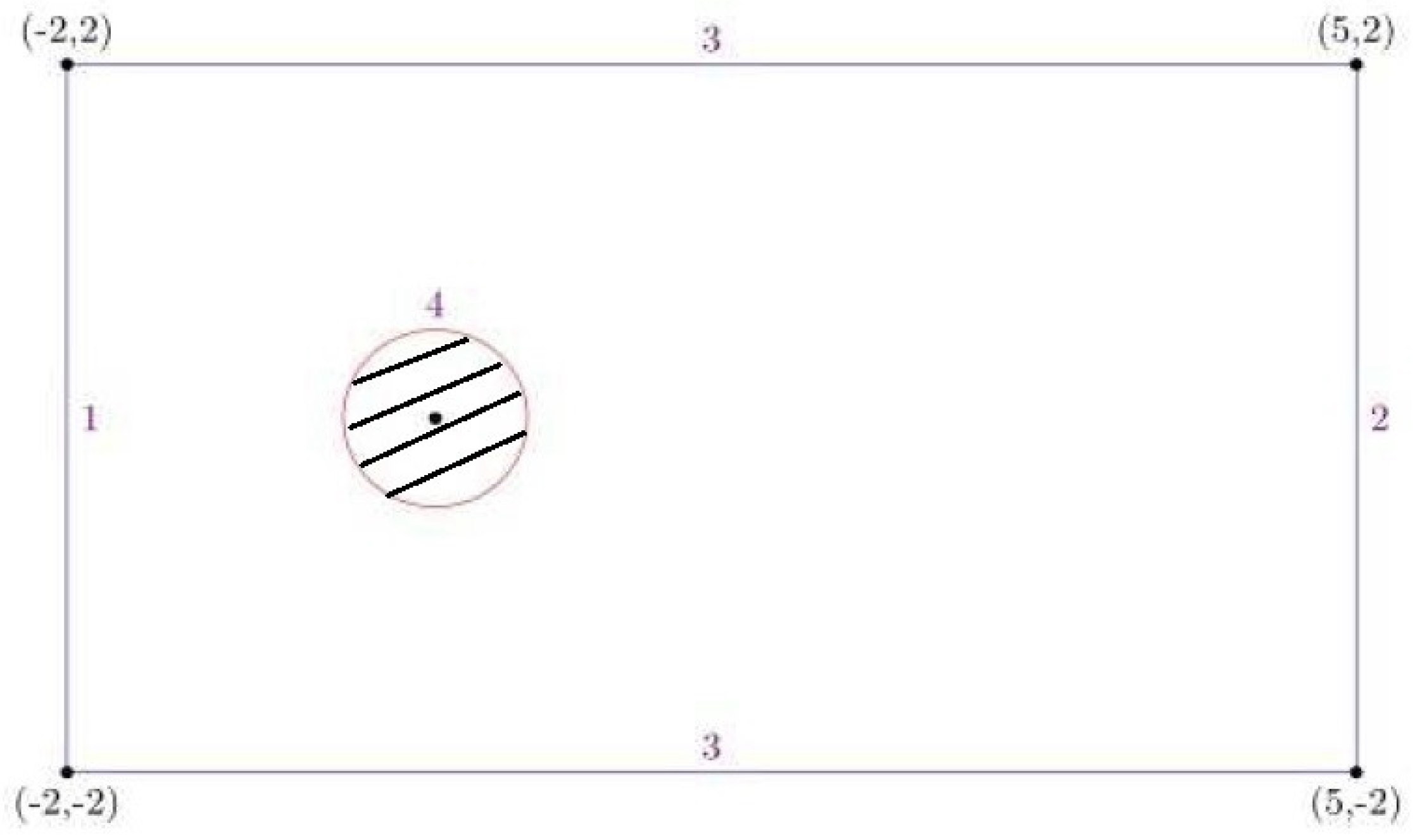
To this end, we assume that the computed domain $\overline{\mathsf{\Omega }}=([-2,5]\times [-2,2])\setminus \{(x,y):x^2+y^2<1\}$ (see Figure 1), Lines 1 and 2 are, respectively, the inlet and outlet boundaries—where the velocity of the x-component is allowed to be freely flowing but the velocity of the y-component is equal to be zero; the upper and lower boundaries (Lines 3), and around cylinder 4 are, respectively, the walls with no-slip flow; the initial velocity and body force vectors are $(u^0,v^0)=(1,0)$ and $(g_1,g_2)=(0,0)$, respectively; the Reynolds number $Re=1000$; and $\Delta t=0.01$, ${\Im }_h$ consists of the right triangles with sides parallel to the coordinate axes with side length $0.0001$, i.e., $h=\sqrt{2}/10,000$, and the FE space consists of the piece-wise linear polynomial. Thus, the theoretical error is $O\left({10}^{-4}\right)$.

We firstly computed 20 CNMFE vorticity solution vectors ${\mathit{\omega }}^n$ ($n=1,2,\cdots ,20$) at the first 20 time-steps on a laptop (Think-Pad E530) and combined the snapshot matrix $\mathit{A}=({\mathit{\omega }}^1,{\mathit{\omega }}^2,\cdots ,{\mathit{\omega }}^{20})$. Then, we found the eigenvalues ${\lambda }_i$$(i=1,2,\cdots ,20)$ of the matrix ${\mathit{A}}^T\mathit{A}$ and the associated eigenvectors ${\mathit{\varphi }}_i$$(i=1,2,\cdots ,20)$. It follows by reckoning that $\sqrt{{\lambda }_7}⩽3\times {10}^{-4}$ so that we only had to choose the first six eigenvectors ${\mathit{\varphi }}_i$$(i=1,2,\cdots ,6)$ to produce the POD basis $\mathsf{\Phi }=({\mathit{\phi }}_1,{\mathit{\phi }}_2,\cdots ,{\mathit{\phi }}_6)$ via the formulas ${\mathit{\phi }}_i=\mathit{A}{\mathit{\varphi }}_i/\sqrt{{\lambda }_i}$$(i=1,2,\cdots ,6)$. In the end, we computed out the RDR-CNMFE velocity solutions $u_d^n$ and $v_d^n$ at $t=5$ on the same laptop (Think-Pad E530) and exhibit them in Figure 2b and Figure 3b, respectively.

In order to exhibit the superiority of RDRMFE method, the CNMFE velocity solutions $u_h^n$ and $v_h^n$ were also computed on the same laptop (Think-Pad E530) and shown in Figure 2a and Figure 3a, respectively. It shown by comparison in each double graph in Figure 2 and Figure 3 that the CNMFE with RDR-CNMFE solutions are basically the same.

In order further to exhibit the superiority of RDR-CNMFE method, we recorded the errors between CNMFE and RDR-CNMFE solutions and the CPU runtime for solving the RDR-CNMFE method and the CNMFE method when $n=200,300,400$, and 500, as listed in

Table 1. Errors between the CNMFE and RDR-CNMFE solutions and CPU runtime.

	$(\mathit{u},\mathit{v})$	CNMFE	RDR-CNMFE
n	Errors	CPU Runtime	CPU Runtime
200	9.2386 × ${10}^{-4}$	482.52143 S	3.27514 S
300	9.4568 × ${10}^{-4}$	723.28654 S	4.76271 S
400	9.6759 × ${10}^{-4}$	964.04126 S	6.55028 S
500	1.0633 × ${10}^{-3}$	1205.96909 S	7.93785 S

. Table 1 shows that the errors between CNMFE and RDR-CNMFE solutions at four time levels, which concur with theoretical errors $O\left({10}^{-4}\right)$, but the RDR-CNMFE method can lessen unknowns and calculating costs, since the RDR-CNMFE method has only $2\times 6$ unknowns at each time-step, whereas the CNMFE method has more than $2\times 28\times {10}^8$ unknowns at the same time-step. Table 1 also shows that the CPU runtime for solving the RDR-CNMFE method is much less than that for solving the CNMFE method, and it is approximately decreased by a factor of 150. Hence, the RDR-CNMFE method is undoubtedly superior to the CNMFE method.

Further, the errors of RDR-CNMFE solutions reach $O\left({10}^{-4}\right)$ (see Figure 4) when $d=6$ and $t=5$. This shows that the numerical results agree with the theoretical ones.

5. Conclusions

We adopted the POD method to study the reduced dimensions for the unknown solution coefficient vectors in the CNMFE method of the 2D unsteady Stokes equation. We constructed the RDR-CNMFE method for the 2D unsteady Stokes equation, and analyzed the existence, stability, and errors for the RDR-CNMFE solutions with matrix analysis. Moreover, we have used some numerical tests to verify the correctness of the theoretical results and also demonstrated that the RDR-CNMFE method is far superior to the CNMFE method, since the unknowns of the RDR-CNMFE method are far fewer than those of the CNMFE method, so that, compared with the CNMFE method, the RDR-CNMFE method can greatly alleviate the calculating burden, mitigate the rounding error accumulation, and shorten the CPU runtime in the calculation process.

What is noteworthy is that the RDR-CNMFE method for the 2D unsteady Stokes equation is constructed only with the initial few solution coefficient vectors of the CNMFE vorticity function such that the construction for the POD bases herein is far simpler and more convenient than that of the existed POD reduced-order methods (see, e.g., [8,9,10,11,12,13,14,15,16,17,18,19,20]). In addition, the construction of the RDR-CNMFE method and the theoretical analysis herein are different from those of the existing POD reduced-order methods. The RDR-CNMFE method for the 2D unsteady Stokes equation is new to this paper and is a completely novel development among the reduced-order methods, since the RDR-CNMFE method has the same basis functions and accuracy as the CNMFE method.

Although we only constructed the RDR-CNMFE method for the 2D unsteady Stokes equation, the approach herein can be extended to the three-dimensional problems or more complex hydrodynamics equations, and can even be applied to solving the more complex real-world engineering problems. Therefore, the method herein has widespread applications.