Tuning Machine Learning Models Using a Group Search Firefly Algorithm for Credit Card Fraud Detection

Abstract

Recent advances in online payment technologies combined with the impact of the COVID-19 global pandemic has led to a significant escalation in the number of online transactions and credit card payments being executed every day. Naturally, there has also been an escalation in credit card frauds, which is having a significant impact on the banking institutions, corporations that issue credit cards, and finally, the vendors and merchants. Consequently, there is an urgent need to implement and establish proper mechanisms that can secure the integrity of online card transactions. The research presented in this paper proposes a hybrid machine learning and swarm metaheuristic approach to address the challenge of credit card fraud detection. The novel, enhanced firefly algorithm, named group search firefly algorithm, was devised and then used to a tune support vector machine, an extreme learning machine, and extreme gradient-boosting machine learning models. Boosted models were tested on the real-world credit card fraud detection dataset, gathered from the transactions of the European credit card users. The original dataset is highly imbalanced; to further analyze the performance of tuned machine learning models, in the second experiment performed for the purpose of this research, the dataset has been expanded by utilizing the synthetic minority over-sampling approach. The performance of the proposed group search firefly metaheuristic was compared with other recent state-of-the-art approaches. Standard machine learning performance indicators have been used for the evaluation, such as the accuracy of the classifier, recall, precision, and area under the curve. The experimental findings clearly demonstrate that the models tuned by the proposed algorithm obtained superior results in comparison to other models hybridized with competitor metaheuristics.

1. Introduction

Since the global pandemic of COVID-19 forced many economies to reevaluate the traditional onsite working environment paradigm, there has been a significant increase in e-commerce and online services based on credit card transactions. The bigger usage of credit cards was followed by an increased number of credit card frauds. This kind of criminal activity occurs when credit card authentication information is stolen with the malicious goal to buy merchandise or services without the owner’s permission or to withdraw money from it. For this reason, it is imperative to implement an effective system to detect fraudulent activity regarding credit card transactions and protect both the users and other institutions affected by this activity.

In this paper, the performance of machine learning (ML) algorithms for detecting credit card frauds, that are compared on a real-world dataset generated from European cardholders during September 2013 from credit card transactions across Europe, are analyzed. However, as can be expected from real-world data, the utilized dataset is extremely imbalanced. In order to deal with the issue of the aforementioned class imbalance, and for the purpose of this research, the use of the synthetic minority over-sampling technique (SMOTE) [1] is proposed, and all methods were also validated against a balanced credit card fraud synthetic dataset. The set of ML algorithms that were evaluated consisted of support vector machine (SVM), extreme learning machine (ELM), and extreme gradient boosting (XGBoost).

It is well-known that every ML model has to be tuned for the specific dataset [2]. This also implies the no free lunch (NFL) theorem, which states that there is no universal approach, nor set of parameters’ values that can render satisfying results for all practical problems. Therefore, un-trainable ML parameters, known in the literature as hyper-parameters, have to be tuned. Moreover, the process of training models can also be an issue, especially for methods that fall into the group of artificial neural networks (ANNs) [3]. Both mentioned ML challenges fall into the category of NP-hard optimization, as it was previously shown they can be tackled with great success by metaheuristic-based techniques [4,5,6].

Therefore, the research proposed in this manuscript first introduces an improved version of widely used firefly algorithm (FA) metaheuristic [7]. The FA belongs to the swarm intelligence family, which is itself a subset of nature-inspired algorithms. The above-mentioned NFL theorem can be applied for optimization algorithms themselves. A single metaheuristic algorithm that can obtain the best results for all optimization problems does not exist. The FA was selected among other metaheuristics empirically, based on the promising results obtained by the original FA version throughout the conducted experiments with various metaheuristic algorithms on this particular optimization problem. Another reason for selecting FA is that it is a well-known metaheuristic that has been established as a powerful optimizer. The proposed method is then used to optimize hyper-parameters of SVM and XGBoost ML models for the practical credit card fraud dataset. Moreover, the introduced metaheuristic was also employed for tuning the number of neurons, as well as for training the ELM model.

The motivation behind this research lies in the fact that the performance of different machine learning classifiers has not been properly investigated in the past for the credit card fraud detection challenge. Additionally, it was also observed that the performance of nature-inspired metaheuristics can be further investigated for ML tuning and training.

Therefore, besides the proposed approach, other recent state-of-the-art swarm intelligence metaheuristics have also been implemented and adapted, and its performance for tuning three ML models for the practical and important credit card fraud detection problem was thoroughly analyzed. In this way, a comprehensive comparative analysis between three ML methods and several metaheuristics is also provided in this manuscript.

Based on the above, the basic research question that guided the experimentation provided in this paper is to test if it is possible to further improve the detection of malevolent credit card activities by employing ML models and to further improve the classification performance of SVM, ELM, and XGBoost methods by tuning them with swarm intelligence.

The main contributions of the proposed research can be summarized as follows.

• The development of the novel improved version of the well-known FA metaheuristic that addresses the known drawbacks of the original implementation.
• The application of the devised algorithm for tuning three machine learning classifiers for the particular task of fraud detection, with a goal to enhance the classifiers’ accuracy, as well as other performance metrics.
• The comprehensive comparative analysis of different swarm intelligence metaheuristics for ML tuning against practical credit card fraud challenge.

The obtained experimental results were subjected to rigid statistical tests to assess their statistical significance and to establish the confidence in the proposed method’s performance level.

The rest of the manuscript is structured as follows: Section 2 briefly introduces the classifiers used in this research and exhibits a survey of swarm intelligence approaches and a variety of their applications. The original FA, the proposed enhanced version, and the ML swarm intelligence framework are presented in Section 3. The conducted experiments are detailed and described in Section 4, together with the experimental setup, utilized dataset, outcomes of the simulations, and comprehensive comparative analysis. Finally, Section 5 winds up the manuscript and puts forward feasible directions for the research that lies ahead.

2. Literature Review and Background

This section first briefly introduces the utilized machine learning classifiers, namely SVM, ELM, and XGBoost. This is followed by a brief survey of swarm intelligence methods and their various practical applications. Finally, the last part of this section discusses various successful classifiers hybridized with swarm intelligence techniques.

2.1. Support Vector Machine

The SVM was proposed in 1995 by Cortes and Vapnik [8]. The SVM classifier is extremely useful when dealing with simple, non-linear data with a high number of dimensions. Nevertheless, it is necessary to perform optimization of its hyper-parameters, including the selection of the proper kernel function, which is an NP-hard computational challenge. With the application of the non-linear transformation, the kernel function can help in constructing the linear decision planes.

Assuming the dataset and the class labels of the $S=x_1,x_2,x_3,$$\cdots x_n$ and $G=y_1,y_2,y_3,$$\cdots y_n$, respectively, SVM searches for the optimal hyperplane H to separate two data-samples and creates the longest interval r between these two samples. This ideal H hyperplane can be stated with Equation (1):

$$W^{T}x+b=0,$$

(1)

where biases are denoted with b, while W corresponds to the weight vector. The challenge is to find optimal b and W, as given by Equation (2):

$$\begin{array}{c}min(\frac{{∥w∥}^2}{2}+C{\displaystyle \sum _{i=1}^l}{\xi }_i)\\ s.t.\left\{\begin{array}{c}{y}_i(w{x}_i+b)\ge 1-{\xi }_i\hfill \\ \xi >0\hfill \end{array}\right.\end{array}$$

(2)

It is possible to reduce Equation (2) to satisfy the Karush Kuhn Tucker (KKT) criterion through the application of Lagrange multipliers. Finally, the objective function can be narrowed down to Equations (3) and (4):

$${max}_a(\sum _{i=1}^l{a}_i-\frac{1}{2}\sum _{i=1}^l\sum _{j=1}^l{y}_i{y}_j{a}_i{a}_j(x_i·x_j))$$

(3)

$$s.t.\sum _{i=1}^l{y}_i{a}_i=0,0\le a_i\le C,$$

(4)

where C is the penalty parameter of the error term. The increase of the C value will give more significance to the range of gap, but it will also increase the danger of generalization, as was observed by performing extensive simulations and analyzing outcomes.

The final linear discriminant function can be represented by Equation (5):

$$f\left(x\right)=sgn(\sum _{i=1}^l{a}^{*}{y}_i(x_i·x)+b^{*}),$$

(5)

where $a^{*}$ is the optimal value of a, and the best values of $w^{*}$ and $b^{*}$ can be calculated as follows:

$$\begin{array}{c}{w}^{*}=\sum _{i=1}^l{a}_i^{*}{x}_i{y}_i\\ b^{*}=-\frac{1}{2}{w}^{*}(x_r+x_s),\end{array}$$

(6)

where $x_r$ and $x_s$ are any pair of support vectors in the two classes.

Taking everything into account, the final classifier function can be formulated as presented in Equation (7):

$$f\left(x\right)=sgn\left\{\begin{array}{c}\left(\sum _{i=1}^n{y}_i{a}_{i}k(x_i·x)\right)+b^{*}\end{array}\right\}$$

(7)

The kernel function can be utilized for splitting the nonlinear data in the linear fashion through translation to a high-dimensional feature search space. The kernel function is given by Equation (8):

$$k(x_i,x)=(\phi \left(x_i\right),\phi \left(x\right))$$

(8)

The Gaussian kernel function is commonly used to address nonlinear high-dimensional data, and its formulation is given by Equation (9):

$$k(x,y)=exp{(-\gamma ∥x-y∥)}^2,$$

(9)

where the $\gamma$ parameter determines how much influence a single training instance has on the final output.

Two most important hyper-parameters that influence the performance of the SVM classifier are C, $\gamma$ and the kernel type.

2.2. Extreme Learning Machine

Extreme learning machine (ELM) is an ML model that has drawn the attention of the research community in recent years. It was initially presented by Huang et al. [9] for single-hidden-layer feed-forward artificial neural networks (SLFNs). The algorithm has shown better generalization performance compared to traditional feed-forward network-learning algorithms while providing great learning speed and efficiency.

The input weights are randomly chosen by the algorithm, after which the output weights of SLFN are analytically determined through a simple generalized inverse operation of the hidden layer output matrices by utilizing the Moore–Penrose (MP) generalized inverse [10]. The classic gradient-based learning algorithms are only able to work for differentiable activation functions. On the other hand, the ELM learning algorithm can be used to train SLFNs with many non-differentiable activation functions. The ELM’s optimization performance mostly depends on an adequate number of neurons in the hidden layer, which is still an open question that ELM models are facing.

For a training sample set ${\left\{(x_j,t_j)\right\}}_{j=1}^N$ with N samples and m classes, the SLFN with L hidden nodes and activation function g(x) is expressed in equation [9]:

$$\sum _{i=1}^L{\beta }_{i}g(w_j·x_j+b_i)=t_j,j=1,2,\dots ,N,$$

(10)

where $w_i={[w_{i1},\dots ,w_{in}]}^T$ is the input weight, $b_i$ is the bias of the i-th hidden node, ${\beta }_i={[{\beta }_{i1},\dots ,{\beta }_{im}]}^T$ is the weight vector which is connecting the ith hidden node and the output nodes, $w_i·x_j$ denotes the inner product of $w_i$ and $x_j$, and $t_j$ is network output with respect to input $x_j$. The Equation (10) can be expressed as:

$$H\beta =T,$$

(11)

where

$$H={\left[\begin{array}{ccc}g(w_1·x_1+b_1)& \cdots & g(w_L·x_1+b_L)\\ ⋮& \cdots & ⋮\\ g(w_1·x_N+b_1)& \cdots & g(w_L·x_N+b_L)\end{array}\right]}_{NxL},\beta ={\left[\begin{array}{c}{\beta }_1^T\\ ⋮\\ {\beta }_L^T\end{array}\right]}_{Lxm},T={\left[\begin{array}{c}t{1}^T\\ ⋮\\ t{N}^T\end{array}\right]}_{Nxm}$$

(12)

In Equation (12), H represents the hidden-layer output matrix of the neural network [11], while $\beta$ is the output weight matrix.

2.3. The XGBoost Algorithm

In order to optimize the objective function, XGBoost algorithm uses the additive training method. This means that each step in the optimization process is dependent on the result from the previous step. The equation for expressing the t-th objective function of XGBoost model is presented below:

$${F_o}^i={\sum }_{k=1}^{n}l\left(y_k,{\widehat{y}}_k^{i-1}+f_i\left(x_k\right)\right)+R\left(f_i\right)+C,$$

(13)

where the loss term of the t-th iteration is denoted as l, C represents a constant term, and R is the regularization parameter of the model, which can be described as:

$$R\left(f_i\right)=\gamma T_i+\frac{\lambda }{2}{\sum }_{j=1}^T{w}_j^2$$

(14)

In general, the larger the values of customization parameters $\gamma$ and $\lambda$ are, the simpler is the structure of the tree. The first g and the second h derivatives of the model can be described with the following equations:

$$g_j={\partial }_{{{\widehat{y}}_k}^{i-1}}l\left(y_j,{{\widehat{y}}_k}^{i-1}\right)$$

(15)

$$h_j={\partial }_{{{\widehat{y}}_k}^{i-1}}^{2}l\left(y_j,{{\widehat{y}}_k}^{i-1}\right)$$

(16)

The solution can be obtained from the next formulas:

$$w_j^{*}=-\frac{\sum g_t}{\sum h_t+\lambda }$$

(17)

$${F_o}^{*}=-\frac{1}{2}\sum _{j=1}^T\frac{{\left(\sum g\right)}^2}{\sum h+\lambda }+\gamma T,$$

(18)

where ${F_o}^{*}$ represents the score of loss function, and $w_j^{*}$ denotes the solution of weights.

2.4. Swarm Intelligence

Swarm intelligence represents the group of optimization algorithms inspirited by the conduct and habits of various sorts of animals in nature [12,13]. Swarm intelligence metaheuristics were modeled by very intelligent food foraging, hunting, and mating techniques expressed by large groups of otherwise rather simple individuals, such as insects, birds, and fish. Consequently, a significant number of metaheuristics emerged and the most notable examples include particle swarm optimization (PSO) [14], artificial bee colony (ABC) [15], firefly algorithm (FA) [7], bat algorithm (BA) [16], elephant herding optimization (EHO) [17], whale optimization algorithm (WOA) [18], dragonfly algorithm (DA) [19], and other popular algorithms [20,21,22,23,24]. Several more recent algorithms also emerged in the last five years, and among the most significant representatives include salp swarm algorithm (SSA) [25], harris’ hawks optimization (HHO) [26], monarch butterfly optimization (MBO) [27], emperor penguin optimizer (EPO) [28], and grasshopper optimization algorithm (GOA) [29].

This family of metaheuristic approaches has been extensively utilized to address numerous practical real-world problems with NP-hard complexity from the domain of heterogeneous real-world domains. Some notable examples of this kind of applications include cloud-edge computing and task scheduling [30,31], wireless sensors networks (WSNs) challenges such as node localization and prolonging the overall lifetime of the network [32,33], healthcare applications and pollution estimation [34], ANNs challenges including feature selection and hyperparameters’ optimization tasks [3,35,36,37,38], cryptocurrency trends estimations [39], computer-guided illness detection [40,41,42], and lastly the occurring COVID-19 global epidemic-associated applications [43,44,45,46].

2.5. Machine Learning Model Tuning by Swarm Intelligence Metaheuristics

The detailed overview of the recent literature shows that the swarm intelligence approaches were not utilized enough to optimize the machine learning models and that there is a lot of open space for research in this direction. This comes as surprise to some extent, especially because metaheuristics have been successfully exploited for numerous other application domains.

One successful swarm intelligence application from this domain worth mentioning is presented in [47], where the implementation of a pair of swarm intelligence algorithms to tune the input weights and biases of ELM (ABC-ELM and IWO-ELM) are implemented. Ref. [48] introduced a hybridized PSO-ELM classifier and validated it for flash flood prediction with very promising results. The SSA-based optimization of ELM was proposed in [49] and put to the test against other contemporary models on 10 standard benchmark datasets, and it proved to be superior in terms of classifier accuracy obtained through simulations. The fruit fly optimization (FFO) algorithm was used in [50] to enhance the SVM performance with significant success. Ref. [39] analyzed the performance of the SVM tuned by enhanced SCA for cryptocurrency trends predictions. Comparisons with traditional models have shown that SCA-based SVM outclassed all competitors for this particular task.

2.6. Credit Card Fraud Detection Overview

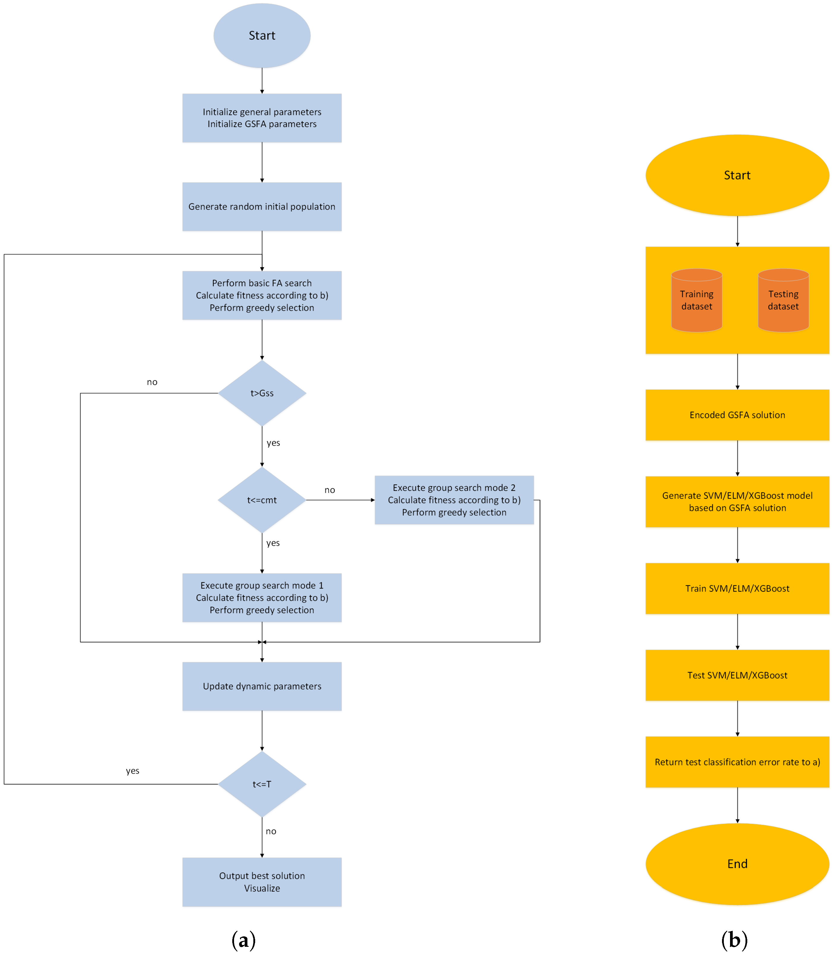
Detecting frauds in credit card transactions is an extremely important task, especially after the COVID-19 outbreak that drastically added to the already increasing number of daily online transactions. The problem with the fraud detection task is the highly imbalanced dataset. Ref. [51] provides an experimental study of various approaches including ANN, SVM, LR, KNN, and NB, among others. The conclusions from this research are clear—although these approaches can be used for solving slightly imbalanced datasets, in cases of extremely imbalanced datasets (such as credit card detection), the obtained results and "high" accuracy can be very misleading, due to the large number of false-positive results, and consequently allow a significant number of frauds to pass without detection. A combination of the supervised and unsupervised learning methods was considered in [52], where the authors implemented and assessed different granularity levels to define an outlier score, however, with unconvincing results. Their conclusions indicate that additional work is required, in terms of various clustering algorithms and feature sets, to validate the proposed method.

The approach proposed in [53] utilized an optimized light gradient-boosting machine to deal with the credit card fraud detection task. The authors have compared their method to the results obtained by other state-of-the-art approaches, including NB, KNN, SVM, and random forest, and were able to conclude that their approach outperforms others on two real-world datasets. Nevertheless, the problem with extremely imbalanced datasets could lead to missed fraud detection. AdaBoost and the majority voting approach were utilized by [54] to address this task, with mixed and varying results. Similar to previous approaches, this method also obtains a near-perfect detecting rate of non-fraud entries; however, it also struggles with fraudulent transactions, again due to the extremely skewed dataset.

The method proposed in [55], which also inspired the research presented in this paper, examines how different machine learning models perform on the credit card dataset that was put into use in this paper as well. The SMOTE method was utilized to address the imbalanced data, and combined traditional classifiers, including random forest, linear regression, SVM, and XGBoost with the AdaBoost technique to examine the impact on classifier accuracy were examined. However, this research did not employ swarm metaheuristics to tune the classifiers.

3. Proposed Method

In this section, the basic FA approach is described first, and afterward, motivations for its improvements along with inner workings details of the proposed enhanced method are provided.

3.1. Original Firefly Algorithm

The firefly algorithm [7] is a swarm intelligence model inspired by the social behavior of fireflies. In the FA metaheuristic, the model for the fitness functions is based on the firefly’s brightness and attraction. In order to simplify a complex system of flashing behavior of the insects, the authors applied several approximation rules. The attraction between the units depends on the brightness, which is determined by the objective function value. The implementation for the problem of minimization is given in equation [7]:

$$I\left(x\right)=\left\{\begin{array}{cc}1/f\left(x\right)\hfill & ,\mathrm{if}f\left(x\right)>0\hfill \\ 1+\left|f\right(x\left)\right|\hfill & ,\mathrm{if}f\left(x\right)\le 0,\hfill \end{array}\right.$$

(19)

in which $I\left(x\right)$ denotes the attractiveness, and $f\left(x\right)$ represents the objective function value at location x.

Furthermore, when the distance is increasing, the intensity of the light is falling, which results in less attraction value [7]:

$$I\left(r\right)={\displaystyle \frac{I_0}{1+\gamma \times r^2}},$$

(20)

where $I\left(r\right)$ is the intensity of the light at the range r, $\gamma$ represents the light absorption coefficient parameter, and $I_0$ is the intensity of light at its source. Most FA implementations combine the effects of the inverse square law for distance and $\gamma$ to approximate the following Gaussian form [7]:

$$I\left(r\right)=I_0·e^{-\gamma \times r^2}$$

(21)

Each firefly unit has attractiveness level $\beta$ which is directly proportional to the level of the firefly’s light factoring in the distance.

$$\beta \left(r\right)={\beta }_0·e^{-\gamma \times r^2},$$

(22)

in which ${\beta }_0$ is attractiveness at distance r = 0. The authors of the original FA suggest that Equation (22) is often swapped for the following equation [7]:

$$\beta \left(r\right)={\beta }_0/\left(1+\gamma \times r^2\right).$$

(23)

Based on Equation (23), the search equation for the random individual i, which is moving in iteration $t+1$ to a new location $x_i$ towards another firefly j with a greater fitness value is [7]:

$$x_i^{t+1}=x_i^t+{\beta }_0·e^{-\gamma \times r_{i,j}^2}(x_j^t-x_i^t)+{\alpha }^t(\kappa -0.5),$$

(24)

where $\alpha$ denotes the randomization parameter, $\kappa$ represents uniform distribution random number, and $r_{i,j}$ is the distance between fireflies i and j. The values for ${\beta }_0$ and $\alpha$ that provide good results are 1 and [0,1], respectively. The $r_{i,j}$ parameter is Cartesian distance and is calculated as follows:

$$r_{i,j}=\Vert x_i-x_j\Vert =\sqrt{{\sum }_{k=1}^D{\left(x_{i,k}-x_{j,k}\right)}^2},$$

(25)

where the parameter D represents the number of parameters of a particular problem.

3.2. Motivation and Proposed Improved Group Search Firefly Algorithm

Previous findings suggest that the basic FA exhibits relatively efficient exploitation, while its exploration abilities can be improved [56,57,58]. Notwithstanding that many successful implementations of enhanced/hybridized FA’s version can be found in the modern literature [31,59], space for its improvements still exists. This stems from the fact that the FA’s search equation, which conducts efficient intensification, can be effectively combined with novel mechanisms, as well as with procedures from other metaheuristics, in a wide variety of ways, and the practical potential for improvements is unlimited.

The enhanced FA’s version proposed in this manuscript tries to overcome the cons of the original implementation by adopting the disputation operator from the recently proposed social network search (SNS) algorithm [60]. This operator practically conducts search process within a chosen group of solutions from the population; therefore, in this study instead of “disputation”, the term “group search” is used.

The disputation phase in the SNS denotes a state where social network users are explaining and defending some views on a given subject with others. Additionally, users may form groups to discuss particular topics. In this way, users are influenced by being able to see various opinions on the same topic. In this phase, a random number of users are observed as commentators or members belonging to a group, and new views are obtained using Equation (26) [60]:

$$\begin{array}{cc}\hfill & x_{inew}=x_i+rand(0,1)\times (M-AF\times x_i)\hfill \\ \hfill & M=\frac{{\sum }_t^{N_r}{x}_t}{Nr}\hfill \\ \hfill & AF=1+round\left(rand\right),\hfill \end{array}$$

(26)

where $x_i$ is the vector denoting the view of $i-th$ user, $rand(0,1)$ is a random vector within range $[0,1]$, and M is the mean of the views of the commentators. The $AF$ represents the admission factor, used to indicate the insistence that the users hold of their opinions while discussing it with others, and it can take only 1 or 2 integer values. Function $round\left(\right)$ is used to round the input to the nearest integer, while $rand$ is an arbitrary number $[0,1]$. Parameter $Nr$ denotes the number of users commenting or the group size. It can have any integer value between 1 and N, where N denotes the total number of network’s users.

Parameter $AF$ is the search step size, and it controls the balance between intensification and diversification. When the $AF$ is adjusted to 2, the exploration is more emphasized, while the value of 1 helps the disputation procedure to conduct more intensive exploitation. In [60], it is explained in many details how the disputation operator executes both exploration and exploitation processes.

However, the method proposed in this research employs a slightly different disputation operator than the one in the SNS metaheuristic; therefore, as pointed out above, instead of disputation, the term “group search” is used throughout this study.

In the SNS approach, the first operand in the $AF$ expression Equation (26) is fixed and set to 1, therefore the $AF$ can only take values of 1 or 2. However, according to conducted empirical studies for the purpose of this research, it is better to set a larger step size at the beginning, this emphasizes exploration, and then gradually decrease it over the course of a run, favoring intensification over diversification. Moreover, to enable fine-tuned search, it is better to allow $AF$ to take continuous value.

Therefore, instead of determining the step size $AF$ according expression Equation (26), the proposed method adapts one more control parameter—the group search parameter ($gsp$), which is dynamic in nature, and the following equation is used for calculating $AF$ in each iteration:

$$AF=gsp+round\left(rand\right),$$

(27)

where the $gsp$ dynamically shrinks in each iteration t according to the following expression, where T denotes the maximum number of iterations in the run:

$$gsp=gsp-\frac{t}{T}$$

(28)

Parameter $gsp$ has an influence on the exploration and exploitation balance by establishing the step size. In the early rounds, the exploration should be dominant; therefore, this parameter has a larger value (in executed experiments, the starting value was set to 2, but it is dynamically decreased over the iterations). Conversely to the SNS algorithm, the proposed method uses a fine-grained step size $AF$, therefore enabling a better directed search.

Additionally, the suggested method adopts two modes of group search. The first mode (mode 1) conducts the search within the group of $N_r$ randomly chosen solutions from the population, while the second mode (mode 2) defines the group as $N_b$ best solutions from the population. $N_r$ and $N_b$ are random numbers between 1 and N, and they are recalculated in each iteration. Both modes utilize Equation (26), while the step size is calculated as shown in Equation (27).

Group search mode 2 is executed in later iterations for performing fine-tuned searches around the current best solutions, with the assumption that the algorithm has converged to the optimum region of the search space. The point in algorithm’s execution when mode 1 is switched to mode 2 is determined by the change mode trigger $cmt$ control parameter, which depends on the termination condition argument.

Most of the previous FAs’ enhanced implementations tackle inadequate exploration drawbacks by incorporating mechanisms that can improve diversification in early iterations [31,61]. However, the method proposed in this study tries an alternate approach. Again, based on empirical findings, if the initial population generated by the FA is near optimum regions, then efficient FA’s search procedure is able to converge fast towards an optimum solution. Conversely, the whole population will converge towards sub-optimum domains of the search space. Therefore, in order to give a chance to the basic FA’s search and not to significantly increase the computational time complexity, instead of triggering the group search in early iterations, the method proposed in this study fires this procedure after the $gss$ (group search start) iterations.

In all iterations, where the conditions for group search triggering are satisfied, a new solution $x_{new}$ is generated, and then the greedy selection between it and the current worst solution $x_{worst}$ is performed.

Inspired by the introduced group search procedure in the basic FA, the proposed method is named group search FA (GSFA). As was shown, the GSFA introduces three new control parameters, out of which one is dynamic. The values of all three parameters depend on the termination condition, which can be either T or the maximum number of fitness function evaluation $FFEs$. The values for these parameters, which are used in simulations, are determined empirically, and they are shown in

Table 1. Specific GSFA parameters’ settings.

Parameter	Expression	Description
$gsp$	$gsp=gsp-\frac{t}{T}$	dynamic group search parameter, starting value 2
$gss$	$gss=\frac{T}{2}$	group search start
$cmt$	$cmt=gss+\frac{T}{3}$	change mode trigger

.

One more thing that is worth mentioning is that the proposed GSFA does not employ a dynamic randomization parameter $\alpha$, as was suggested in some of the previous studies [58]. Experiments with a dynamic randomization parameter were also conducted, and it was concluded that if dynamic $\alpha$ is employed, then the search process in the early iterations (before the group search is triggered) would converge too fast towards the unpromising solution; therefore, at the end of a run, worse solutions would be produced.

The computation complexity of the original FA algorithm in terms of $FFEs$ can be retrieved from [62]. When compared to the basic FA, the complexity of the proposed GSFA is higher for only $(T-gss)$$FFEs$, because, after the group search is triggered, only one new solution is generated in each iteration. This was taken into consideration in the comparative analysis to maintain fair comparison conditions.

Finally, the GSFA pseudo-code is depicted in Algorithm 1.

Algorithm 1 The GSFA pseudo-code.

Define global parameters N and T Generate the initial population of solutions $x_i$, ($i=1,2,3,\dots N$) Define basic FA control parameters Define specific GSFA control parameters Set initial values of dynamic parameters while$t<T$do    for $i=1$ to N do      for $j=1$ to i do         if $I_j<I_i$ then           Move the firefly j in the direction of the firefly i in D dimension           Attractiveness changes with distance r as exp[$-\gamma r$]           Evaluate the new solution, replace the worst solution with better one and update intensity of light         end if      end for    end for    Sort population according to fitness in descending order and determine solution with index -1 ($x_{worst}$)    if $t>gss$ then      if $t<cmt$ then         Generate new solution $x_{new}$ by group search mode 1 operator      else         Generate new solution $x_{new}$ by group search mode 2 operator      end if      Perform greedy selection between $x_{new}$ and $x_{worst}$    end if    All solution are ranked in order to find the current best solution end while Output the global best solution $x^{*}$ Post-process results and perform visualization

4. Experimental Findings, Comparative Analysis, and Discussion

This section opens with description of the dataset that was employed in the simulations, along with the experimental setup details. Afterwards, this section brings forward the outcomes of the simulations with extensive comparative analysis and findings discussion.

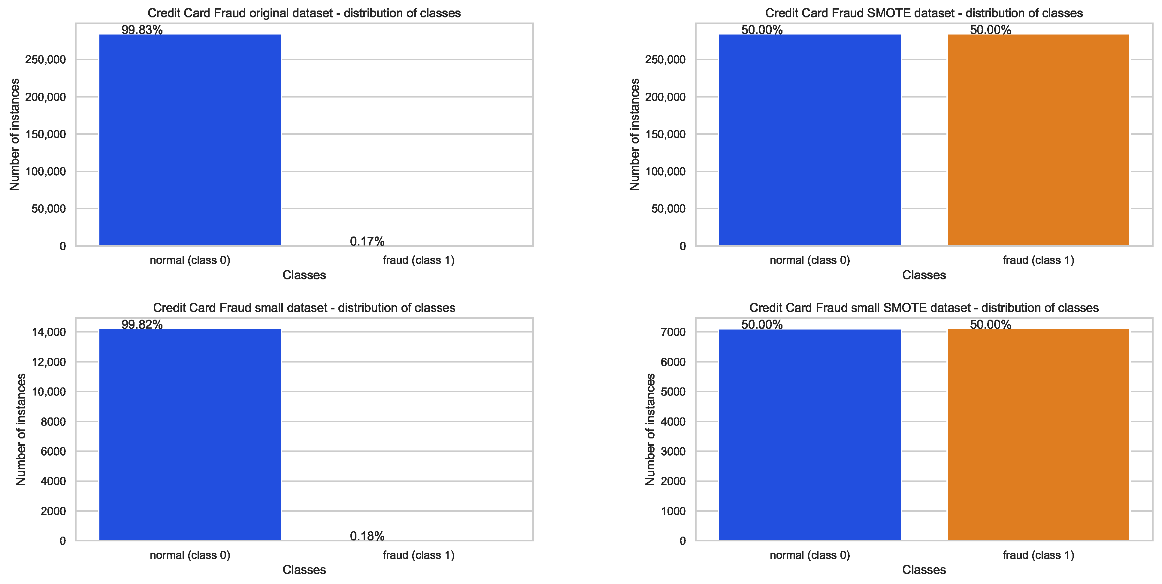
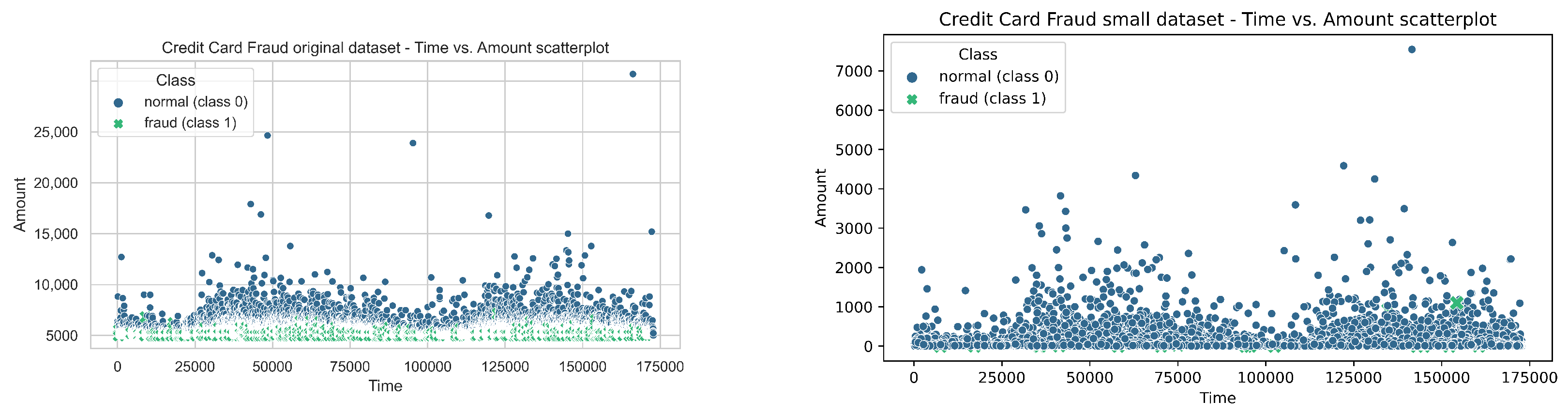
4.1. Datasets Used in Experiments

All simulations were executed against the credit card fraud dataset, which is freely available on the Kaggle repository via the following link: https://www.kaggle.com/datasets/mlg-ulb/creditcardfraud, accessed on 20 May 2022. This dataset consists of transactions generated by credit cards in Europe in September 2013 during the time span of two days. The dataset represents a binary classification challenge composed of only two target variables (classes)—the positive class, which denotes fraudulent transactions and the negative class that represents regular transactions. Moreover, the dataset is extremely asymmetrical (imbalanced) containing only 492 fraud instances out of 284,807 total transactions. Therefore, the positive class (frauds) represent only 0.172% of the dataset.

The dataset is composed of 30 numerical features, where attributes $F1,F2,\cdots F28$ are obtained by applying the principal component analysis (PCA), while $F29$ and $F30$, which represent time and amount, respectively, were not transformed with the PCA. The time refers to the number of seconds elapsed between the first and each other transaction in the dataset, while the amount is the value of every transaction.

In the first set of experiments, the original credit card fraud dataset, as it is hosted on the Kaggle, is used, and the goal of these experiments was to establish how tuned ML models perform on highly imbalanced data. However, since it is also important to validate the performance of ML models for balanced datasets, the SMOTE methodology [1] has been applied to tackle the extreme disproportion of class instances in the observed dataset in the second set of experiments. The SMOTE operates by generating new entries of the given class through data-point connection with K-nearest neighbors. In this way, additional synthetic entries are generated without replicating them directly from the minority class instances, thus avoiding the over-fitting issue throughout model training. In the proposed study, the minority class (class 1 in this example) was over-sampled to the number of instances of the majority category (class 0 in this example); therefore, the dataset, which in addition to the original also contains a synthetic data point for the minority class, is almost twice as large as the original one.

It needs to be noted that the experimental setup for SVM simulations had to be different, due to the specific properties of the model. In the case of SVM, a smaller dataset has been used, as the model operates very slowly. This was tackled by creating a reduced dataset with the size of only 0.5% of the original dataset that was fed to other models while keeping the original class distribution (by using the stratification strategy). The SMOTE dataset for SVM was generated as a random sampling 0.25% of the original SMOTE dataset; therefore, both datasets for SVM consist of approximately 14,216 instances. To differentiate between the employed datasets, the small dataset used to validate SVM performance is denoted with the suffix ‘small’.

In the case of SVM and ELM experiments, the normalization technique was also used. However, since the XGBoost operates on a decision tree basis, normalization has not been performed in that case. A total of 70% of each dataset was used for training, while the remaining 30% was utilized for testing of all models.

The number of instances and class distribution of all four datasets used in this study are shown in Figure 1.

Additionally, the correlation between the features time and amount, which were not subjected to the PCA, with the hue set to class, for original and small datasets, is shown in Figure 2. In order to emphasize the fraudulent transactions, the marker size for class 1 is set as four times bigger than the size for class 0.

4.2. Experimental Setup, Proposed Encoding Scheme, and Flow-Chart Diagram

As noted previously, all three ML models were tuned by the proposed GSFA metaheuristic. In the case of the first utilized model, namely the SVM, three hyper-parameters were subjected to optimization, two of them are continuous, while one is of the integer data type. The optimized SVM parameters, along with respective lower and upper bounds, are as follows:

• C, boundaries: $[2^{-5},2^{15}]$, type: continuous,
• $\gamma$, boundaries: $[2^{-15},2^3]$, type: continuous, and
• kernel type, boundaries: $[0,3]$, type: integer, where value 0 denotes polynomial (poly), 1 marks radial basis function (rbf), 2 represents sigmoid, and finally 3 represents linear kernel type.

For the ELM model, both the number of neurons ($nn$) in the hidden layer and the values of the weights and biases between the input and hidden layers were subjected to the optimization process. The lower and upper bounds for weights and biases were set as −1 and 1, respectively, while the search space boundary for the $nn$ was set as the interval $[30,150]$. The $nn$ is an integer, while the weights and biases may take any continuous value from the specified range.

Moreover, since $nn$ is ELM’s hyper-parameters, while the optimization of weights and biases is the ELM’s training process, in the case of ELM, metaheuristics were used for both hyper-parameters’ optimization and training.

Finally, the set of XGBoost hyper-parameters that were subjected to optimization consists of the following:

• learning rate ($\eta$), boundaries: $[0.1,0.9]$, type: continuous,
• $min\_child\_weight$, boundaries: $[0,10]$, type: continuous,
• subsample, boundaries: $[0.01,1]$,type: continuous,
• collsample_bytree, boundaries: $[0.01,1]$, type: continuous,
• max_depth, boundaries: $[3,10]$, type: integer and
• $gamma$, boundaries: $[0,0.5]$, type: continuous.

The number of parameters for softprob objective function (’num_class’:self.no_classes) is also passed as the parameter to XGBoost. All other parameters are fixed and take default XGBoost values.

All observed models were implemented in the Python programming language, by employing standard machine learning libraries: scikit-learn, scipy, numpy as pandas. For other models’ hyper-parameters, the default values from the scikit-learn Python library were used. The SVM and XGBoost models were adopted from scikit-learn; however, the ELM was coded from scratch because this model is not available in this package.

In all implementations, a standard solutions’ encoding scheme was used. Every metaheuristic solution is represented as an array (vector) of size l, where l is the number of hyper-parameters that were optimized. Therefore, the l for the SVM and XGBoost solutions’ are 3 and 6, respectively.

However, in the case of ELM, l depends on the determined value for the $nn$ hyper-parameter, and, if the $fs$ denotes the size of input feature vector, it can be derived as: $1+nn·fs+nn$. The first component of the ELM metaheuristic solution represents the number of neurons (integer); subsequent $nn$ components are biases (continuous), while remaining $nn·fs$ parameters are weights.

A flow-chart diagram of proposed methodology used in simulations is depicted in Figure 3.

Based on the above image, tuning all three machine learning models represent mixed continuous and integer NP-hard challenges. The fitness of the GSFA solution is simply the classification error rate obtained for the test dataset; therefore, the problem is formulated as a minimization challenge.

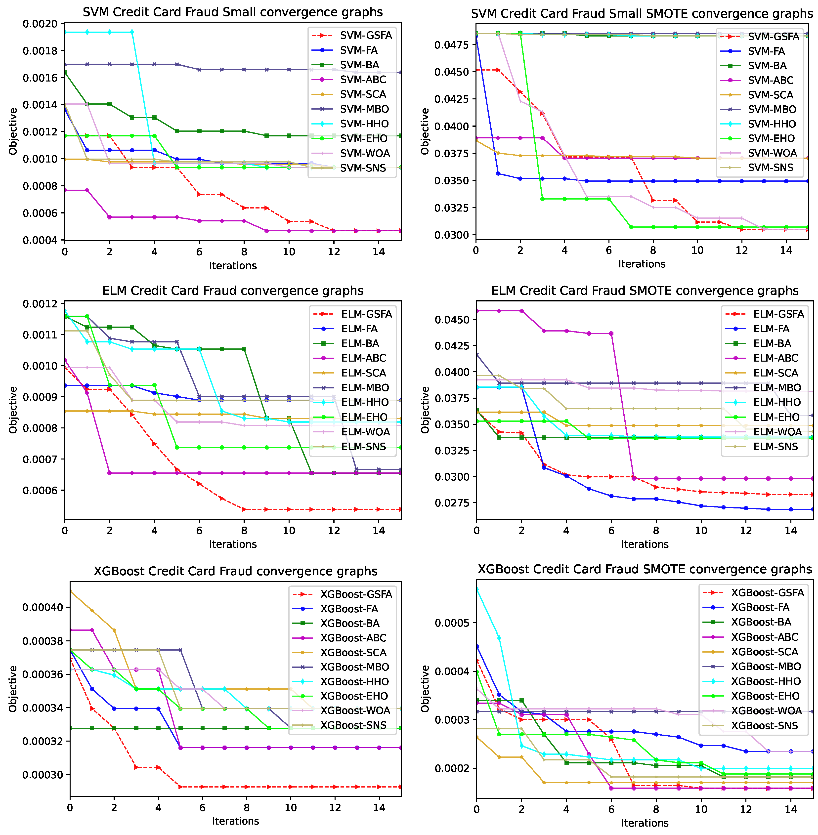
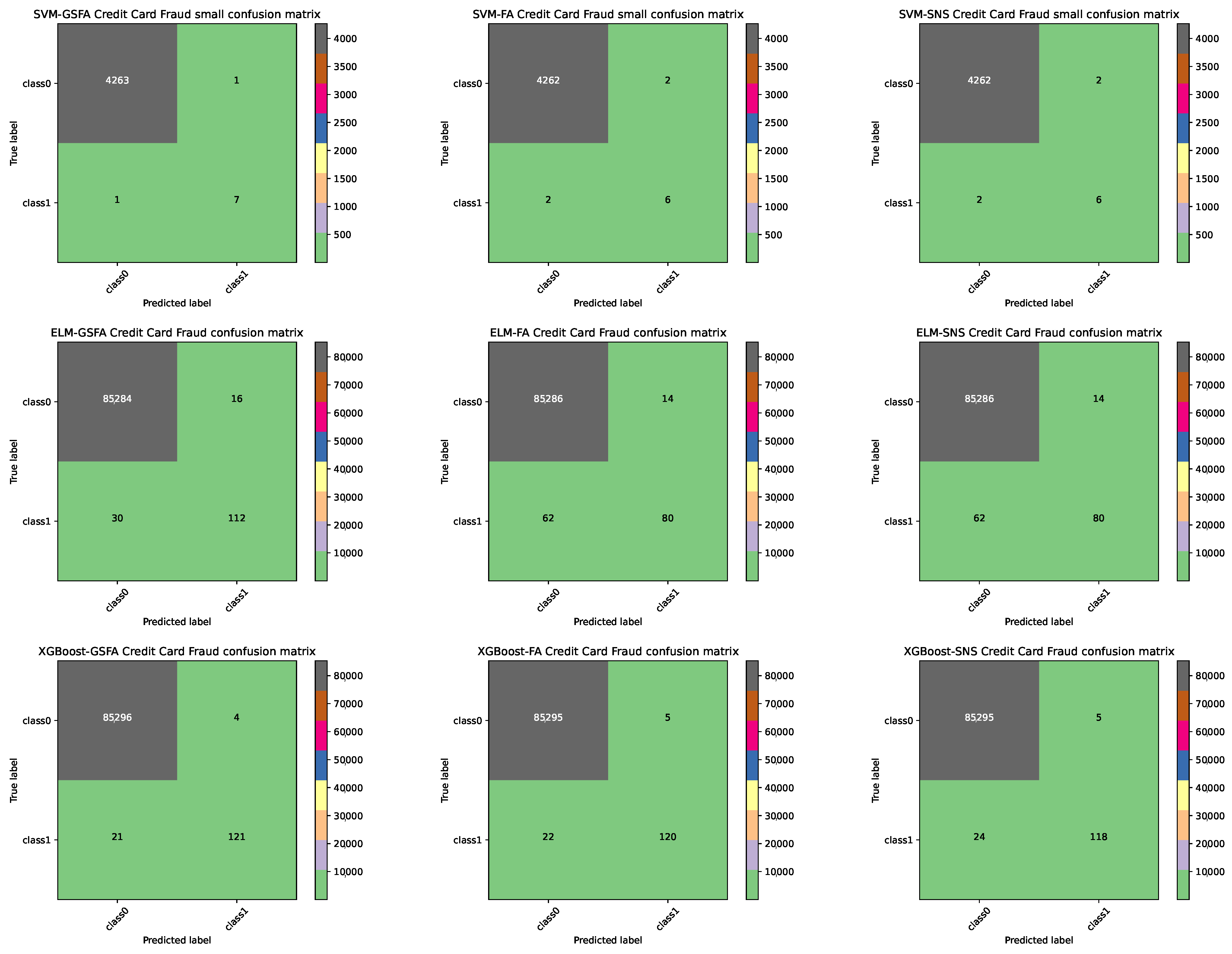
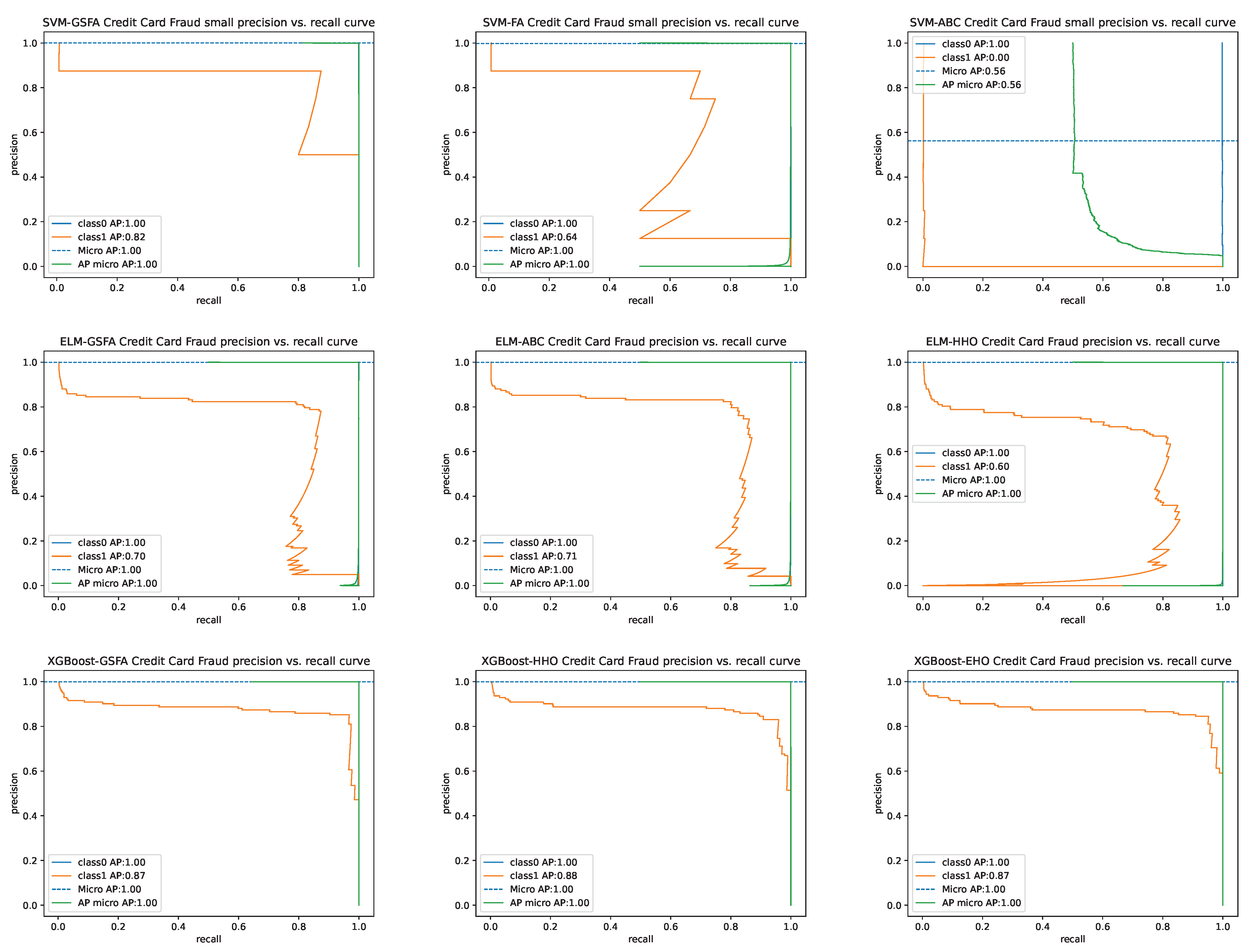
4.3. Comparative Analysis and Discussion

In all experiments, the obtained outcomes of all three models optimized by the suggested GSFA metaheuristic were compared to the results generated by other well-known swarm algorithms that were also implemented for the SVM, ELM, and XGBoost model tuning under the same conditions, as described in Section 4.2. The competitor algorithms include the original FA [7], BA [63], ABC [15], since cosine algorithm (SCA) [64], MBO [27], HHO [26], EHO [17], WOA [18], and SNS [60]. All metaheuristics were implemented independently in this research and adjusted (in terms of controls’ parameters setup) as in the original publications that were mentioned beforehand. For the easier summary of results presented in tables, the machine learning model prefix is placed in front of the methods’ names used for hyper-parameters optimization, e.g., SVM-GSFA denotes the results obtained by SVM classifier tuned with the proposed GSFA method.

The simulations were executed with 20 solutions in the population ($N=20$) and 15 iterations in each run ($T=15$) for each metaheuristic method, except for the GSFA and FA. Since the FA in each iteration in average case performs $2·N$ solutions’ evaluations, in this case N was set to 10. Additionally, due to the slightly higher complexity of the proposed GSFA over the basic FA, the GSFA was tested with only nine solutions. This reduction of the population for the FA and GSFA methods was required to set firm grounds for fair comparisons. Specific GSFA parameters ($gsp$, $gss$ and $cmt$) were set according to Table 1.

All swarm algorithms were also implemented in Python, and Intel^® Core™ i9-11900K Processor with 64 GB of RAM and Windows 11 O.S. was used as a simulation platform. All employed datasets were relatively large, and the cache argument for SVM and XGBoost models in scikit-learn environment was set to 32 GB to improve the computation speed. On the other hand, the ELM is implemented by using the cupy instead of numpy library for operations with matrices, because the cupy supports execution on GPU, and, in this case, NVIDIA Geforce GTX 1080 GPU with 8 GB of memory is employed for such computations.

Due to the stochastic nature of swarm approaches, all methods were executed in 50 independent runs, and best, worst, mean, and median accuracies along with standard deviation are recorded. However, accuracy may not be an objective metric, especially for imbalanced datasets; therefore, precision, recall, and f1-score per class and micro-averaged are also shown along with receiver operating characteristic area under the curve (ROC AUC). It is noted that, in all results tables, the best-achieved metrics are denoted in bold style.

Table 2. SVM Credit Card Fraud small NO SMOTE—general metrics.

Metrics	SVM-GSFA	SVM-FA	SVM-BA	SVM-ABC	SVM-SCA	SVM-MBO	SVM-HHO	SVM-EHO	SVM-WOA	SVM-SNS
best (%)	99.9552	99.9064	99.8830	99.9532	99.9064	99.8361	99.9064	99.9064	99.9064	99.9064
worst (%)	99.9064	99.8596	99.8596	99.9064	99.9064	99.8127	99.9064	99.8127	99.9064	99.8596
mean (%)	99.9220	99.8752	99.8674	99.9298	99.9064	99.8283	99.9064	99.8752	99.9064	99.8908
median (%)	99.9064	99.8596	99.8596	99.9298	99.9064	99.8361	99.9064	99.9064	99.9064	99.9064
std	0.000270	0.000270	0.000135	0.000234	0.000000	0.000135	0.000000	0.000541	0.000000	0.000270

depicts the outcomes of the experiments with the SVM model without the SMOTE technique employed. As was already mentioned, the SVM model is specific due to its slow operation, and the reduced dataset was used. In this particular scenario, the SVM-GSFA achieved the best accuracy result, while the SVM-ABC obtained slightly better mean and median values. However, neither SVM-GSFA, nor SVM-ABC exhibited best robustness, which can be noticed from std metrics, while SVM-WOA, SVM-HHO and SVM-SCA did not show results variation over different runs.

On the other hand,

Table 3. ELM Credit Card Fraud NO SMOTE—general metrics.

Metrics	ELM-GSFA	ELM-FA	ELM-BA	ELM-ABC	ELM-SCA	ELM-MBO	ELM-HHO	ELM-EHO	ELM-WOA	ELM-SNS
best (%)	99.9462	99.9111	99.9345	99.9345	99.9169	99.9333	99.9181	99.9263	99.9192	99.9111
worst (%)	99.9427	99.8841	99.9134	99.8947	99.9029	99.8982	99.8947	99.9075	99.9075	99.8947
mean (%)	99.9442	99.8947	99.9207	99.9058	99.9105	99.9099	99.9081	99.9160	99.9160	99.9029
median (%)	99.9438	99.8917	99.9175	99.8970	99.9111	99.9040	99.9099	99.9151	99.9157	99.9029
std	0.000018	0.000123	0.000095	0.000192	0.000059	0.000163	0.000109	0.000077	0.000136	0.000070

shows the outcomes of the simulations with the ELM model against the dataset without SMOTE. In this scenario, the novel ELM-GSFA model outperformed all other hybrid ELM frameworks for all performance indicators, including best, worst, mean, and median classification accuracy, as well as the stability of results expressed with standard deviation.

Table 4. XGBoost Credit Card Fraud NO SMOTE—general metrics.

Metrics	XGBoost-GSFA	XGBoost-FA	XGBoost-BA	XGBoost-ABC	XGBoost-SCA	XGBoost-MBO	XGBoost-HHO	XGBoost-EHO	XGBoost-WOA	XGBoost-SNS
best (%)	99.9707	99.9684	99.9672	99.9684	99.9661	99.9672	99.9661	99.9672	99.9661	99.9661
worst (%)	99.9696	99.9649	99.9625	99.9661	99.9649	99.9649	99.9649	99.9649	99.9661	99.9637
mean (%)	99.9704	99.9668	99.9649	99.9668	99.9653	99.9664	99.9657	99.9657	99.9661	99.9649
median (%)	99.9707	99.9672	99.9649	99.9661	99.9649	99.9672	99.9661	99.9649	99.9661	99.9649
std	0.000007	0.000018	0.000023	0.000014	0.000007	0.000014	0.000007	0.000014	0.000000	0.000012

puts forward the outcomes of the experiments with XGBoost classifier on real dataset (without SMOTE). Similarly to the previous scenario, the XGBoost-GSFA achieved the best accuracy results for all utilized metrics and outperformed all other competitor methods.

Table 5. SVM Credit Card Fraud small with the SMOTE—general metrics.

Metrics	SVM-GSFA	SVM-FA	SVM-BA	SVM-ABC	SVM-SCA	SVM-MBO	SVM-HHO	SVM-EHO	SVM-WOA	SVM-SNS
best (%)	96.9519	96.5064	95.1700	96.2954	96.2954	95.1465	95.1700	96.9285	96.9519	95.1700
worst (%)	96.8039	96.2704	94.0674	96.0005	95.9408	94.6151	94.1505	96.2706	96.4701	94.3300
mean (%)	96.8643	96.3557	94.4115	96.0875	96.0431	94.8514	94.4080	96.6505	96.6271	94.9307
median (%)	96.8504	96.3691	94.5049	96.0651	96.0251	94.8352	94.3261	96.5141	96.7155	94.9480
std	0.001050	0.007410	0.056500	0.002150	0.008980	0.010500	0.045500	0.007450	0.006660	0.074500

presents the outcomes of the experiments with SVM model on synthetic dataset. In this case, the SVM-GSFA and SVM-WOA were tied for the best accuracy result (96.9519%), while the SVM-GSFA achieved better mean and median values, as well as better stability than opponent algorithms. For the next scenario,

Table 6. ELM Credit Card Fraud with the SMOTE—general metrics.

Metrics	ELM-GSFA	ELM-FA	ELM-BA	ELM-ABC	ELM-SCA	ELM-MBO	ELM-HHO	ELM-EHO	ELM-WOA	ELM-SNS
best (%)	97.1716	97.3140	96.6270	97.0186	96.5133	96.4165	96.6229	96.6364	96.1867	96.5695
worst (%)	97.1046	97.2455	96.4971	97.0046	96.3211	96.3961	96.4708	96.5071	95.8648	96.3695
mean (%)	97.1440	97.2669	96.5881	97.0126	96.3971	96.4055	96.5207	96.6044	96.0175	96.4710
median (%)	97.1595	97.261	96.5794	97.0069	96.4671	96.4087	96.4981	96.5951	96.0266	96.4898
std	0.000321	0.000355	0.004440	0.000456	0.000059	0.000429	0.084200	0.025200	0.023600	0.003450

shows the results of the simulations for the ELM model with the SMOTE dataset. In this scenario, the ELM-FA model outperformed all other hybrid ELM solutions for all performance indicators, including best, worst, mean, and median classification accuracies, as well as the standard deviation, while the novel ELM-GSFA obtained second-best results. Finally,

Table 7. XGBoost Credit Card Fraud with the SMOTE—general metrics.

Metrics	XGBoost-GSFA	XGBoost-FA	XGBoost-BA	XGBoost-ABC	XGBoost-SCA	XGBoost-MBO	XGBoost-HHO	XGBoost-EHO	XGBoost-WOA	XGBoost-SNS
best (%)	99.9842	99.9766	99.9818	99.9842	99.9830	99.9683	99.9818	99.9812	99.9766	99.9818
worst (%)	99.9841	99.9740	99.9786	99.9803	99.9810	99.9642	99.9793	99.9762	99.9743	99.9756
mean (%)	99.9841	99.9750	99.9800	99.9836	99.9823	99.9662	99.9800	99.9795	99.9757	99.9794
median (%)	99.9841	99.9751	99.9801	99.9841	99.9824	99.9669	99.9801	99.9786	99.9756	99.9786
std	0.000001	0.000020	0.000095	0.000034	0.000034	0.000072	0.000084	0.000085	0.000067	0.000105

puts forward the findings of simulations with XGBoost classifier with synthetic data generated by SMOTE technique. The XGBoost-GSFA and XGBoost-ABC were tied for the best and median accuracy results, while XGBoost-GSFA finished first for worst, mean and standard deviation indicators.

For better visual representation, convergence speed graphs for all swarm intelligence algorithms used in the analysis and for all three ML models are shown in Figure 4. From the presented graphs, it is clear that the GSFA outperforms all other metaheuristics, including the original FA in all cases except ELM simulations with the SMOTE dataset, in terms of convergence speed. Additionally, the GSFA manages to converge substantially faster than the SNS algorithm.

Table 8. SVM Credit Card Fraud small NO SMOTE—detailed metrics.

	Metrics
Metaheuristic	Accuracy (%)	Precision 0	Precision 1	M.Avg. Precision	Recall 0	Recall 1	M.Avg. Recall	F1 Score 0	F1 Score 1	M.Avg. F1 Score	M.Avg. ROC AUC	M.Avg. PR AUC
SVM-GSFA	99.9532	0.999765	0.875000	0.999532	0.999765	0.875000	0.999532	0.999765	0.875000	0.999532	1.00	1.00
SVM-FA	99.9064	0.999531	0.750000	0.999064	0.999531	0.750000	0.999064	0.999531	0.750000	0.999064	1.00	1.00
SVM-BA	99.8830	0.999063	0.800000	0.998690	0.999765	0.500000	0.998830	0.999414	0.615385	0.998695	1.00	1.00
SVM-ABC	99.9532	0.998251	0.002015	0.996385	0.535413	0.500000	0.535346	0.696993	0.004014	0.695695	0.52	0.56
SVM-SCA	99.9064	0.999531	0.750000	0.999064	0.999531	0.750000	0.999064	0.999531	0.750000	0.999064	1.00	1.00
SVM-MBO	99.8361	0.998127	0.000000	0.996258	0.999765	0.000000	0.997893	0.998946	0.000000	0.997075	0.50	0.50
SVM-HHO	99.9064	0.999531	0.750000	0.999064	0.999531	0.750000	0.999064	0.999531	0.750000	0.999064	1.00	1.00
SVM-EHO	99.9064	0.999297	0.833333	0.998986	0.999765	0.625000	0.999064	0.999531	0.714286	0.998997	1.00	1.00
SVM-WOA	99.9064	0.999531	0.750000	0.999064	0.999531	0.750000	0.999064	0.999531	0.750000	0.999064	1.00	1.00
SVM-SNS	99.9064	0.999531	0.750000	0.999064	0.999531	0.750000	0.999064	0.999531	0.750000	0.999064	1.00	1.00

,

Table 9. ELM Credit Card Fraud NO SMOTE—detailed metrics.

	Metrics
Metaheuristic	Accuracy (%)	Precision 0	Precision 1	M.Avg. Precision	Recall 0	Recall 1	M.Avg. Recall	F1 Score 0	F1 Score 1	M.Avg. F1 Score	M.Avg. ROC AUC	M.Avg. PR AUC
ELM-GSFA	99.9462	0.999648	0.875000	0.999441	0.999812	0.788732	0.999462	0.999730	0.829630	0.999448	1.00	1.00
ELM-FA	99.9111	0.999274	0.851064	0.999027	0.999836	0.563380	0.999111	0.999555	0.677966	0.999020	1.00	1.00
ELM-BA	99.9345	0.999637	0.816176	0.999332	0.999707	0.781690	0.999345	0.999672	0.798561	0.999338	1.00	1.00
ELM-ABC	99.9345	0.999555	0.852459	0.999310	0.999789	0.732394	0.999345	0.999672	0.787879	0.999320	1.00	1.00
ELM-SCA	99.9169	0.999332	0.858586	0.999098	0.999836	0.598592	0.999169	0.999584	0.705394	0.999095	1.00	1.00
ELM-MBO	99.9333	0.999578	0.834646	0.999304	0.999754	0.746479	0.999333	0.999666	0.788104	0.999314	1.00	1.00
ELM-HHO	99.9181	0.999402	0.827273	0.999116	0.999777	0.640845	0.999181	0.999590	0.722222	0.999129	1.00	1.00
ELM-EHO	99.9263	0.998338	0.000000	0.996679	1.000000	0.000000	0.998338	0.999168	0.000000	0.997508	0.50	0.50
ELM-WOA	99.9192	0.999391	0.841121	0.999128	0.999801	0.633803	0.999192	0.999596	0.722892	0.999136	1.00	1.00
ELM-SNS	99.9111	0.999274	0.851064	0.999027	0.999836	0.563380	0.999111	0.999555	0.677966	0.999020	1.00	1.00

and

Table 10. XGBoost Credit Card Fraud NO SMOTE—detailed metrics.

	Metrics
Metaheuristic	Accuracy (%)	Precision 0	Precision 1	M.Avg. Precision	Recall 0	Recall 1	M.Avg. Recall	F1 Score 0	F1 Score 1	M.Avg. F1 Score	M.Avg. ROC AUC	M.Avg. PR AUC
XGBoost-GSFA	99.9707	0.999754	0.968000	0.999701	0.999953	0.852113	0.999707	0.999853	0.906367	0.999698	1.00	1.00
XGBoost-FA	99.9684	0.999742	0.960000	0.999676	0.999941	0.845070	0.999684	0.999842	0.898876	0.999674	1.00	1.00
XGBoost-BA	99.9672	0.999730	0.959677	0.999664	0.999941	0.838028	0.999672	0.999836	0.894737	0.999661	1.00	1.00
XGBoost-ABC	99.9684	0.999742	0.960000	0.999676	0.999941	0.845070	0.999684	0.999842	0.898876	0.999674	1.00	1.00
XGBoost-SCA	99.9661	0.999719	0.959350	0.999652	0.999941	0.830986	0.999661	0.999830	0.890566	0.999648	1.00	1.00
XGBoost-MBO	99.9672	0.999730	0.959677	0.999664	0.999941	0.838028	0.999672	0.999836	0.894737	0.999661	1.00	1.00
XGBoost-HHO	99.9661	0.999719	0.959350	0.999652	0.999941	0.830986	0.999661	0.999830	0.890566	0.999648	1.00	1.00
XGBoost-EHO	99.9672	0.999742	0.952381	0.999663	0.999930	0.845070	0.999672	0.999836	0.895522	0.999663	1.00	1.00
XGBoost-WOA	99.9661	0.999730	0.952000	0.999651	0.999930	0.838028	0.999661	0.999830	0.891386	0.999650	1.00	1.00
XGBoost-SNS	99.9661	0.999719	0.959350	0.999652	0.999941	0.830986	0.999661	0.999830	0.890566	0.999648	1.00	1.00

provide additional detailed results for other significant machine learning performance metrics, including per-class and micro-averaged precision, recall, and F1 Score, along with ROC AUC for the experiments where models were employed without SMOTE technique. On the other hand,

Table 11. SVM Credit Card Fraud small with the SMOTE—detailed metrics.

	Metrics
Metaheuristic	Accuracy (%)	Precision 0	Precision 1	M.Avg. Precision	Recall 0	Recall 1	M.Avg. Recall	F1 Score 0	F1 Score 1	M.Avg. F1 Score	M.Avg. ROC AUC	M.Avg. PR AUC
SVM-GSFA	96.9519	0.945285	0.996530	0.970913	0.996717	0.942335	0.969520	0.970320	0.968675	0.969497	0.99	0.99
SVM-FA	96.5064	0.943228	0.989151	0.966195	0.989681	0.940459	0.965064	0.965896	0.964191	0.965043	0.99	0.99
SVM-BA	95.1700	0.911891	1.000000	0.955956	1.000000	0.903422	0.951700	0.953915	0.949261	0.951587	0.99	0.98
SVM-ABC	96.2954	0.931381	0.999494	0.965446	0.999531	0.926394	0.962954	0.964253	0.961557	0.962905	1.00	1.00
SVM-SCA	96.2954	0.931381	0.999494	0.965446	0.999531	0.926395	0.962954	0.964253	0.961557	0.962905	1.00	1.00
SVM-MBO	95.1465	0.536780	0.533067	0.534923	0.506567	0.563057	0.534818	0.521236	0.547652	0.534447	0.54	0.53
SVM-HHO	95.1700	0.911891	1.000000	0.955956	1.000000	0.903422	0.951700	0.953915	0.949261	0.951587	0.99	0.98
SVM-EHO	96.9285	0.946054	0.995054	0.970560	0.995310	0.943272	0.969285	0.970057	0.968472	0.969264	0.99	0.99
SVM-WOA	96.9519	0.946875	0.994568	0.970727	0.994841	0.944210	0.969519	0.970265	0.968735	0.969500	0.99	0.99
SVM-SNS	95.1700	0.911891	1.000000	0.955956	1.000000	0.903422	0.951700	0.953915	0.949261	0.951587	0.99	0.98

,

Table 12. ELM Credit Card Fraud with the SMOTE—detailed metrics.

	Metrics
Metaheuristic	Accuracy (%)	Precision 0	Precision 1	M.Avg. Precision	Recall 0	Recall 1	M.Avg. Recall	F1 Score 0	F1 Score 1	M.Avg. F1 Score	M.Avg. ROC AUC	M.Avg. PR AUC
ELM-GSFA	97.1716	0.961894	0.982012	0.971931	0.982475	0.960909	0.971716	0.972076	0.971346	0.971712	1.00	1.00
ELM-FA	97.3140	0.967921	0.978501	0.973200	0.978837	0.967418	0.973140	0.973349	0.972928	0.973139	1.00	1.00
ELM-BA	96.6270	0.966703	0.965835	0.966270	0.965957	0.966584	0.966270	0.966330	0.966209	0.966270	0.99	0.99
ELM-ABC	97.0186	0.958294	0.982770	0.970506	0.983294	0.957020	0.970186	0.970633	0.969724	0.970180	0.99	0.99
ELM-SCA	96.5133	0.948796	0.982790	0.965755	0.983493	0.946692	0.965132	0.965833	0.964403	0.965119	0.99	0.99
ELM-MBO	96.4165	0.949218	0.980219	0.964685	0.980966	0.947291	0.964165	0.964831	0.963474	0.964154	0.99	0.99
ELM-HHO	96.6229	0.952841	0.980501	0.966641	0.981165	0.951227	0.966229	0.966796	0.965642	0.966220	0.99	0.99
ELM-EHO	96.6364	0.957048	0.976114	0.966560	0.976708	0.955974	0.966364	0.966778	0.965939	0.966359	0.99	0.99
ELM-WOA	96.1867	0.958182	0.965630	0.961898	0.966062	0.957654	0.961867	0.962106	0.961626	0.961866	0.99	0.99
ELM-SNS	96.5695	0.960938	0.970575	0.965746	0.971011	0.960357	0.965695	0.965948	0.965439	0.965694	0.99	0.99

and

Table 13. XGBoost Credit Card Fraud with the SMOTE—detailed metrics.

	Metrics
Metaheuristic	Accuracy (%)	Precision 0	Precision 1	M.Avg. Precision	Recall 0	Recall 1	M.Avg. Recall	F1 Score 0	F1 Score 1	M.Avg. F1 Score	M.Avg. ROC AUC	M.Avg. PR AUC
XGBoost-GSFA	99.9842	0.999988	0.999695	0.999842	0.999696	0.999988	0.999842	0.999842	0.999841	0.999842	1.00	1.00
XGBoost-FA	99.9766	0.999965	0.999565	0.999766	0.999567	0.999965	0.999766	0.999766	0.999765	0.999766	1.00	1.00
XGBoost-BA	99.9818	0.999988	0.999648	0.999818	0.999649	0.999988	0.999818	0.999819	0.999818	0.999818	1.00	1.00
XGBoost-ABC	99.9842	0.999965	0.999718	0.999842	0.999719	0.999965	0.999842	0.999842	0.999841	0.999842	1.00	1.00
XGBoost-SCA	99.9830	0.999965	0.999695	0.999830	0.999696	0.999965	0.999830	0.999830	0.999830	0.999830	1.00	1.00
XGBoost-MBO	99.9683	0.999941	0.999425	0.999684	0.999427	0.999941	0.999683	0.999684	0.999683	0.999683	1.00	1.00
XGBoost-HHO	99.9818	0.999965	0.999671	0.999818	0.999672	0.999965	0.999818	0.999819	0.999818	0.999818	1.00	1.00
XGBoost-EHO	99.9812	0.999965	0.999660	0.999812	0.999661	0.999965	0.999812	0.999813	0.999812	0.999812	1.00	1.00
XGBoost-WOA	99.9766	0.999930	0.999601	0.999766	0.999602	0.999930	0.999766	0.999766	0.999765	0.999766	1.00	1.00
XGBoost-SNS	99.9818	0.999977	0.999659	0.999818	0.999661	0.999976	0.999818	0.999819	0.999818	0.999818	1.00	1.00

present the same metrics for the simulations where models were tested against the dataset with the SMOTE approach.

The yielded detailed metrics provide significant insights into the algorithms’ performance, especially for imbalanced datasets such as credit card fraud without the SMOTE technique. From the reported metrics, it can be unequivocally confirmed that, on average, when all models are taken into account, the proposed GSFA algorithm proved that it is able to achieve the best classification performance for a minority class (class 1 in this example).

The generated confusion matrices for the original credit card fraud dataset by tuned SVM, ELM, and XGBoost models with GSFA, FA, and SNS algorithms are shown in Figure 5, while precision–recall (PR) curve graphs for GSFA and arbitrary chosen approaches for synthetic dataset are depicted in Figure 6.

Lastly, the hyper-parameters’ values for the tuned SVM, ELM, and XGBoost models, generated in the best run for each applied optimization algorithm, are shown in

Table 14. Best SVM parameters’ values obtained by the analyzed algorithms.

Method/Parameters		No SMOTE			With SMOTE
	C	$\mathit{\gamma }$	Kernel Type	C	$\mathit{\gamma }$	Kernel Type
SVM-GSFA	1816.0411	0.0492	1	0.031	0.1015	0
SVM-FA	16316.8042	$3\times {10}^{-5}$	0	0.031	1.6601	1
SVM-BA	32768	0.1172	2	2106.3912	7.6593	0
SVM-ABC	6064.1918	0.0142	1	8512.3559	$3\times {10}^{-5}$	2
SVM-SCA	15,430.8553	$3\times {10}^{-5}$	0	8591.6538	$3\times {10}^{-5}$	2
SVM-MBO	14,167.7370	1.9988	2	631.3854	5.1329	0
SVM-HHO	22,160.9077	$3\times {10}^{-5}$	0	500.4590	2.3178	0
SVM-EHO	0.031	2.3360	0	2425.9645	0.0234	0
SVM-WOA	22,320.8262	$3\times {10}^{-5}$	0	0.0353	0.0912	0
SVM-SNS	32,768	$3\times {10}^{-5}$	0	8277.7914	0.6790	0

,

Table 15. Best ELM number of neurons in hidden layer obtained by the analyzed algorithms.

Method/	No SMOTE	With SMOTE
Parameters	Number of Neurons	Number of Neurons
ELM-GSFA	88	67
ELM-FA	60	74
ELM-BA	30	85
ELM-ABC	85	86
ELM-SCA	53	150
ELM-MBO	97	135
ELM-HHO	50	48
ELM-EHO	56	79
ELM-WOA	64	133
ELM-SNS	64	90

and

Table 16. Best XGBoost parameters’ values obtained by the analyzed algorithms.

Method/		No SMOTE
Parameters	eta	min_child_weight	Subsample	colsample_bytree	max_depth	Gamma
XGBoost-GSFA	0.6109	5.3438	0.6276	0.7093	8.0268	0.4437
XGBoost-FA	0.8330	7.1837	0.9261	0.7303	3.7943	0.1307
XGBoost-BA	0.7028	6.7516	0.6247	0.6904	5.7910	0.3833
XGBoost-ABC	0.8340	7.7698	0.5957	0.7957	6.2033	0.0021
XGBoost-SCA	0.5143	1.5846	1	0.7242	6.6324	0.4547
XGBoost-MBO	0.6572	3.9720	0.5423	0.7891	5.3727	0.1232
XGBoost-HHO	0.6329	2.2029	0.9299	0.9118	7.8752	0.5
XGBoost-EHO	0.6274	10	1	0.6247	5.1698	0.5
XGBoost-WOA	0.5940	5.5582	0.5548	0.6715	6.0848	0.4435
XGBoost-SNS	0.6841	1	0.9168	1	5.8061	0.1113
		With SMOTE
Parameters	eta	min_child_weight	Subsample	colsample_bytree	max_depth	Gamma
XGBoost-GSFA	0.8753	5.5543	0.9998	0.7219	9.5889	0.3941
XGBoost-FA	0.7744	5.7581	0.9646	0.4266	8.9161	0.0730
XGBoost-BA	0.8889	1	1	0.4705	9.9235	0.3647
XGBoost-ABC	0.8581	3.9509	0.7588	0.3775	10	0.0874
XGBoost-SCA	0.9	1	0.9368	0.5866	10	0
XGBoost-MBO	0.7940	2.1121	0.4077	0.7334	8.7939	0.2791
XGBoost-HHO	0.8227	5.0387	0.9566	0.4330	9.6767	0.4883
XGBoost-EHO	0.9	3.9113	0.8527	0.7699	10	0.5
XGBoost-WOA	0.8606	2.5538	0.9666	0.9613	9.5649	0.1993
XGBoost-SNS	0.9	1	0.8993	0.5963	10	0.0858

, respectively. It should be noted that Table 15 depicts just the number of neurons $nn$ parameter that obtained the best results, as showing all weights and biases parameters would not be feasible.

4.4. Statistical Tests

Since the experimental outcomes are typically not sufficient to state that one algorithm has better performance when compared to other competitors, contemporary computer science practice requires researchers to establish whether or not the obtained improvements are statistically significant. In the research suggested in this manuscript, 10 methods (including proposed GSFA) were validated for SVM, ELM, and XGBoost tuning against the original (highly imbalanced) and synthetic, generated using the SMOTE technique (balanced) on credit card fraud datasets. Therefore, 10 methods were compared against 6 problem instances, which falls into the domain of multiple approaches for multi-problem analysis [65].

According to the recommendations from the literature [65,66,67], statistical tests in such scenarios may be conducted by constructing a results sample for each approach by taking averages of the measured objectives over multiple independent runs for each problem. However, this approach may have disadvantages when the measured variable has outliers that do not follow a normal distribution, which may lead to deceptive conclusions. According to a literature survey, whether the average objective function value should be taken for the purpose of statistical tests when comparing stochastic methods still remains an open question [65].

For the purpose of comparing 10 methods for 6 problem instances, despite the above-noted potential disadvantages, the objective function (classification error rate) was averaged over 50 independent runs is used in statistical tests. However, this decision was rendered based on the conducted Shapiro–Wilk [68] test for single-problem analysis [65] in the following way: for each algorithm and every problem, a data sample is constructed by taking the results obtained in each run, and respective p-values are calculated for every method–problem pair. The obtained p-values for this test are shown in

Table 17. Shapiro–Wilk test results for single-problem analysis.

	Methods
Problem	GSFA	FA	BA	ABC	SCA	MBO	HHO	EHO	WOA	SNS
SVM	$6.15\times {10}^{-1}$	$4.24\times {10}^{-1}$	$7.05\times {10}^{-1}$	$4.37\times {10}^{-1}$	$8.29\times {10}^{-1}$	$6.02\times {10}^{-1}$	$7.40\times {10}^{-1}$	$4.40\times {10}^{-1}$	$1.23\times {10}^{-1}$	$4.23\times {10}^{-1}$
SVM Smote	$8.06\times {10}^{-1}$	$7.49\times {10}^{-1}$	$5.82\times {10}^{-1}$	$4.92\times {10}^{-1}$	$3.05\times {10}^{-1}$	$5.93\times {10}^{-1}$	$8.08\times {10}^{-1}$	$3.63\times {10}^{-1}$	$3.33\times {10}^{-1}$	$4.51\times {10}^{-1}$
ELM	$6.37\times {10}^{-1}$	$5.32\times {10}^{-1}$	$6.52\times {10}^{-1}$	$5.30\times {10}^{-1}$	$8.42\times {10}^{-2}$	$6.05\times {10}^{-1}$	$5.55\times {10}^{-1}$	$2.84\times {10}^{-1}$	$2.85\times {10}^{-1}$	$8.52\times {10}^{-2}$
ELM Smote	$1.56\times {10}^{-1}$	$9.46\times {10}^{-2}$	$4.52\times {10}^{-1}$	$6.95\times {10}^{-1}$	$1.34\times {10}^{-1}$	$1.12\times {10}^{-1}$	$8.58\times {10}^{-2}$	$3.50\times {10}^{-1}$	$7.92\times {10}^{-1}$	$3.10\times {10}^{-1}$
XGB	$7.98\times {10}^{-1}$	$4.24\times {10}^{-1}$	$9.52\times {10}^{-2}$	$7.35\times {10}^{-1}$	$7.29\times {10}^{-1}$	$7.49\times {10}^{-1}$	$5.32\times {10}^{-1}$	$6.93\times {10}^{-1}$	$6.07\times {10}^{-1}$	$7.43\times {10}^{-1}$
XGB Smote	$3.94\times {10}^{-1}$	$3.84\times {10}^{-1}$	$1.75\times {10}^{-1}$	$5.23\times {10}^{-1}$	$4.01\times {10}^{-1}$	$5.69\times {10}^{-1}$	$6.66\times {10}^{-1}$	$7.24\times {10}^{-1}$	$5.21\times {10}^{-1}$	$5.62\times {10}^{-1}$

.

The results from Table 17 indicate that all p-values are higher than the threshold significance level $\alpha =0.05$, yielding the conclusion that the null hypothesis cannot be rejected; therefore, the data samples for all method–problem pairs originate from a normal distribution, and it is safe to use average objective in the statistical tests.

From this point, we proceeded with multi-problems multiple methods statistical analysis, and the data sample for each method was constructed by taking the average objective function value over 50 independent runs for each problem instance.

First, the safe use of the parametric tests conditions, which include independence, normality, and homoscedasticity of the variances of the data, were checked [69]. The condition of independence was satisfied, because each run was executed independently starting with unique pseudo-random number seed. To check normality, the Shapiro–Wilk test [68] was used again. The results for every method are reported in

Table 18. Shapiro–Wilk test results for multiple problem analysis.

	Methods
	GSFA	FA	BA	ABC	SCA	MBO	HHO	EHO	WOA	SNS
p-value	$3.20\times {10}^{-3}$	$8.34\times {10}^{-3}$	$9.71\times {10}^{-3}$	$6.81\times {10}^{-3}$	$3.28\times {10}^{-3}$	$9.19\times {10}^{-3}$	$8.90\times {10}^{-3}$	$2.32\times {10}^{-3}$	$4.58\times {10}^{-3}$	$8.34\times {10}^{-3}$

.

Finally, to check homoscedasticity based on means, Levene’s test [70] is employed, and the p-value of 0.64 is obtained, which follows that the homoscedasticity is satisfied. However, the rendered p-values from the Shapiro–Wilk test for all methods are smaller than $\alpha =0.05$ (Table 18), yielding the conclusion that the safe use of parametric tests is not satisfied, and we proceeded with non-parametric tests. In all non-parametric tests, the proposed GSFA was established as the control method.

Consequently, the Friedman test [71,72] and a wo-way variance analysis by ranks were utilized to establish the significance of the proposed GSFA performance over other algorithms. The use of this test for multiple methods—multi-problem analysis along with associated Holm post-hoc procedure—was suggested in [66]. The Friedman test results are reported in

Table 19. Friedman test ranks for the compared algorithms.

Functions	GSFA	FA	BA	ABC	SCA	MBO	HHO	EHO	WOA	SNS
SVM	1	7.5	9	2	4	10	4	7.5	4	6
SVM Smote	1	4	9	5	6	8	10	2	3	7
ELM	1	10	2	8	4	6	7	3	5	9
ELM Smote	2	1	4	6	9	8	5	3	10	7
XGB	1	2.5	9.5	2.5	8	4	6.5	6.5	5	9.5
XGB Smote	1	7	4	2	3	10	9	8	6	5
Average Ranking	1.17	5.33	6.25	4.25	5.67	7.67	6.92	5.00	5.50	7.25
Rank	1	4	7	2	6	10	8	3	5	9

. Moreover, the Friedman aligned test was also conducted, and these findings are shown in

Table 20. Friedman aligned test ranks for the compared algorithms.

Functions	GSFA	FA	BA	ABC	SCA	MBO	HHO	EHO	WOA	SNS
SVM	9	46.5	49	11	13	50	13	46.5	13	24
SVM Smote	1	5	59	7	8	58	60	2	3	57
ELM	10	48	16	43	35	38	40	21	36	44
ELM Smote	6	4	42	52	55	54	51	15	56	53
XGB	20	25.5	32.5	25.5	31	27	29.5	29.5	28	32.5
XGB Smote	17	37	22	18	19	45	41	39	34	23
Average Ranking	10.50	27.67	36.75	26.08	26.83	45.33	39.08	25.50	28.33	38.92
Rank	1	5	7	3	4	10	9	2	6	8

.

The findings from Table 19 statistically suggest that the proposed GSFA method obtained superior performance in comparison to other algorithms by achieving an average rank value of 1.17. The second-best result was achieved by ABC, with an obtained average rank of 4.25. The original FA accomplished an average ranking of 5.33; therefore, the superiority of the proposed GSFA over original method is obvious. Additionally, the Friedman statistics (${\chi }_r^2=21.27$) are greater than the ${\chi }^2$ critical value, with 9 degrees of freedom ($16.9$), at significance level $\alpha =0.05$, and the Friedman p-value is $4.55\times {10}^{-8}$, inferring that significant differences in results between different methods exist. Consequently, it is possible to reject the null hypothesis ($H_0$) and state that the proposed GSFA obtained performance were significantly different from other competitors. Similar conclusions can be derived from the Friedman aligned test results.

Additionally, as stated in reference [73], which indicates that the Iman and Davenport’s test [74] could give results with more precision than the ${\chi }^2$, this test was performed as well. The Iman and Davenport’s test result is $3.25\times {10}^0$, which is significantly larger than the critical value of the F-distribution ($2.09\times {10}^0$). Additionally, the Iman and Devenport p-value is $5.32\times {10}^{-2}$, which is smaller than the level of significance. Finally, it is concluded that this test also rejects $H_0$.

Due to the fact that both tests rejected the null hypothesis, the non-parametric post-hoc Holm’s step-down procedure was applied, and the outcomes are given in

Table 21. Results of the Holm’s step-down procedure.

Comparison	p-Value	Rank	0.05/($\mathit{k}-\mathit{i}$)	0.1/($\mathit{k}-\mathit{i}$)
GSFA vs. MBO	$1.00\times {10}^{-4}$	0	0.005556	0.011111
GSFA vs. SNS	$2.51\times {10}^{-4}$	1	0.006250	0.012500
GSFA vs. HHO	$5.02\times {10}^{-4}$	2	0.007143	0.014286
GSFA vs. BA	$1.82\times {10}^{-3}$	3	0.008333	0.016667
GSFA vs. SCA	$5.02\times {10}^{-3}$	4	0.010000	0.020000
GSFA vs. WOA	$6.59\times {10}^{-3}$	5	0.012500	0.025000
GSFA vs. FA	$8.57\times {10}^{-3}$	6	0.016667	0.033333
GSFA vs. EHO	$1.42\times {10}^{-2}$	7	0.025000	0.050000
GSFA vs. ABC	$3.89\times {10}^{-2}$	8	0.050000	0.100000

. In this process, the observed algorithms are sorted in respect of their p values and evaluated to $\alpha /(k-i)$, where k and i denote the degree of freedom ($k=9$ for this research) and the algorithm number, respectively, after sorting in respect to the p value in ascending order (corresponding to rank). This research utilizes $\alpha$ values of 0.05 and 0.1 in this experiment. The findings from Table 21 clearly indicate that the suggested GSFA significantly outperformed all competitors at both significance levels.

5. Conclusions

The research presented in this paper proposed a novel variant of the famous FA algorithm, named GSFA metaheuristic, with an aim to address the notable drawbacks of the original implementation. The introduced GSFA approach adopts a disputation operator from the recently proposed SNS metaheuristic.

The suggested GSFA was paired with three standard ML models, namely the SVM, ELM, and XGBoost models, to perform hyper-parameter optimization. This challenge is still an open question in the ML domain, because every ML model has to be tuned for a specific dataset.

The suggested hybrid model’s performance was verified against the credit card fraud detection dataset, which includes transactions gathered across Europe in 2013. The employed dataset is highly disproportional, as the majority of entries represent valid transactions, and just a small portion mark the fraudulent actions.

The performances of the proposed GSFA-optimized SVM, ELM, and XGBoost were compared to nine other metaheuristics-optimized variants of ML models. The competitor metaheuristics encompassed well-known algorithms, such as the original implementation of FA, BA, ABC, SCA, MBO, HHO, EHO, WOA, and SNS. The experiments were conducted in two phases: first with the original imbalanced dataset and second with a synthetic dataset generated by SMOTE technique. The SMOTE was utilized to generate additional synthetic minority instances and to mitigate the high level of disproportion between the classes. The outcomes of the executed simulations indicate the superior performances of the proposed GSFA for most of the test instances. Finally, rigid statistical tests were performed to confirm the significance of the obtained test results.

Therefore, in the proposed research, it was shown that the FA metaheuristic can be further improved and that the tuned SVM, ELM, and XGBoost models achieve decent performance for a highly challenging and important credit card fraud dataset.

However, the proposed study also has some limitations. First,the GSFA metaheuristic employs three additional control parameters that need to be adjusted for each particular NP-hard challenge. Moreover, the performance of the algorithm needs to be further evaluated for other NP-hard challenges.

The future trials of the suggested GSFA algorithm will include further testing on supplementary real-life credit card datasets. Another direction for validating the proposed GSFA is to apply it and test it on other NP-hard problems, falling into the domains of cloud computing, cryptocurrencies forecasting, and image processing and classification.

References

1. Elreedy, D.; Atiya, A.F. A Comprehensive Analysis of Synthetic Minority Oversampling Technique (SMOTE) for handling class imbalance. Inf. Sci. 2019, 505, 32–64. [Google Scholar] [CrossRef]
2. Nematzadeh, S.; Kiani, F.; Torkamanian-Afshar, M.; Aydin, N. Tuning hyperparameters of machine learning algorithms and deep neural networks using metaheuristics: A bioinformatics study on biomedical and biological cases. Comput. Biol. Chem. 2022, 97, 107619. [Google Scholar] [CrossRef] [PubMed]
3. Bacanin, N.; Bezdan, T.; Venkatachalam, K.; Zivkovic, M.; Strumberger, I.; Abouhawwash, M.; Ahmed, A. Artificial Neural Networks Hidden Unit and Weight Connection Optimization by Quasi-Refection-Based Learning Artificial Bee Colony Algorithm. IEEE Access 2021, 9, 169135–169155. [Google Scholar] [CrossRef]
4. Bacanin, N.; Bezdan, T.; Tuba, E.; Strumberger, I.; Tuba, M. Optimizing Convolutional Neural Network Hyperparameters by Enhanced Swarm Intelligence Metaheuristics. Algorithms 2020, 13, 67. [Google Scholar] [CrossRef] [Green Version]
5. Al-Andoli, M.; Tan, S.C.; Cheah, W.P. Parallel stacked autoencoder with particle swarm optimization for community detection in complex networks. Appl. Intell. 2022, 52, 3366–3386. [Google Scholar] [CrossRef]
6. Gajic, L.; Cvetnic, D.; Zivkovic, M.; Bezdan, T.; Bacanin, N.; Milosevic, S. Multi-layer Perceptron Training Using Hybridized Bat Algorithm. In Computational Vision and Bio-Inspired Computing; Smys, S., Tavares, J.M.R.S., Bestak, R., Shi, F., Eds.; Springer: Singapore, 2021; pp. 689–705. [Google Scholar]
7. Yang, X.S. Firefly Algorithms for Multimodal Optimization. In Stochastic Algorithms: Foundations and Applications; Watanabe, O., Zeugmann, T., Eds.; Springer: Berlin/Heidelberg, Germany, 2009; pp. 169–178. [Google Scholar]
8. Cortes, C.; Vapnik, V. Support-vector networks. Mach. Learn. 1995, 20, 273–297. [Google Scholar] [CrossRef]
9. Huang, G.B.; Zhu, Q.Y.; Siew, C.K. Extreme learning machine: A new learning scheme of feedforward neural networks. In Proceedings of the IEEE International Joint Conference on Neural Networks (IEEE Cat. No.04CH37541), Budapest, Hungary, 25–29 July 2004; Volume 2, pp. 985–990. [Google Scholar] [CrossRef]
10. Serre, D. Matrices: Theory and Applications; Springer: Berlin/Heidelberg, Germany, 2002. [Google Scholar]
11. Huang, G.B. Learning capability and storage capacity of two-hidden-layer feedforward networks. IEEE Trans. Neural Netw. 2003, 14, 274–281. [Google Scholar] [CrossRef] [Green Version]
12. Raslan, A.F.; Ali, A.F.; Darwish, A. 1—Swarm intelligence algorithms and their applications in Internet of Things. In Swarm Intelligence for Resource Management in Internet of Things; Intelligent Data-Centric Systems; Academic Press: Cambridge, MA, USA, 2020; pp. 1–19. [Google Scholar] [CrossRef]
13. Rostami, M.; Berahmand, K.; Nasiri, E.; Forouzandeh, S. Review of swarm intelligence-based feature selection methods. Eng. Appl. Artif. Intell. 2021, 100, 104210. [Google Scholar] [CrossRef]
14. Kennedy, J.; Eberhart, R. Particle swarm optimization. In Proceedings of the ICNN’95—International Conference on Neural Networks, Perth, WA, Australia, 27 November–1 December 1995; Volume 4, pp. 1942–1948. [Google Scholar] [CrossRef]
15. Karaboga, D.; Basturk, B. On the performance of artificial bee colony (ABC) algorithm. Appl. Soft Comput. 2008, 8, 687–697. [Google Scholar] [CrossRef]
16. Yang, X.; Hossein Gandomi, A. Bat algorithm: A novel approach for global engineering optimization. Eng. Comput. 2012, 29, 464–483. [Google Scholar] [CrossRef] [Green Version]
17. Wang, G.G.; Deb, S.; Coelho, L.d.S. Elephant Herding Optimization. In Proceedings of the 3rd International Symposium on Computational and Business Intelligence (ISCBI), Bali, Indonesia, 7–9 December 2015; pp. 1–5. [Google Scholar] [CrossRef]
18. Mirjalili, S.; Lewis, A. The Whale Optimization Algorithm. Adv. Eng. Softw. 2016, 95, 51–67. [Google Scholar] [CrossRef]
19. Mirjalili, S. Dragonfly algorithm: A new meta-heuristic optimization technique for solving single-objective, discrete, and multi-objective problems. Neural Comput. Appl. 2016, 27, 1053–1073. [Google Scholar] [CrossRef]
20. Dorigo, M.; Birattari, M. Ant Colony Optimization. In Encyclopedia of Machine Learning; Springer US: Boston, MA, USA, 2010; pp. 36–39. [Google Scholar] [CrossRef]
21. Mucherino, A.; Seref, O. Monkey search: A novel metaheuristic search for global optimization. AIP Conf. Proc. 2007, 953, 162–173. [Google Scholar] [CrossRef]
22. Mirjalili, S.; Mirjalili, S.M.; Lewis, A. Grey Wolf Optimizer. Adv. Eng. Softw. 2014, 69, 46–61. [Google Scholar] [CrossRef] [Green Version]
23. Gandomi, A.H.; Yang, X.S.; Alavi, A.H. Cuckoo search algorithm: A metaheuristic approach to solve structural optimization problems. Eng. Comput. 2013, 29, 17–35. [Google Scholar] [CrossRef]
24. Yang, X.S. Flower Pollination Algorithm for Global Optimization. In Unconventional Computation and Natural Computation; Springer: Berlin/Heidelberg, Germany, 2012; pp. 240–249. [Google Scholar]
25. Mirjalili, S.; Gandomi, A.H.; Mirjalili, S.Z.; Saremi, S.; Faris, H.; Mirjalili, S.M. Salp Swarm Algorithm: A bio-inspired optimizer for engineering design problems. Adv. Eng. Softw. 2017, 114, 163–191. [Google Scholar] [CrossRef]
26. Heidari, A.A.; Mirjalili, S.; Faris, H.; Aljarah, I.; Mafarja, M.; Chen, H. Harris hawks optimization: Algorithm and applications. Future Gener. Comput. Syst. 2019, 97, 849–872. [Google Scholar] [CrossRef]
27. Wang, G.G.; Deb, S.; Cui, Z. Monarch butterfly optimization. Neural Comput. Appl. 2019, 31, 1995–2014. [Google Scholar] [CrossRef] [Green Version]
28. Dhiman, G.; Kumar, V. Emperor penguin optimizer: A bio-inspired algorithm for engineering problems. Knowl.-Based Syst. 2018, 159, 20–50. [Google Scholar] [CrossRef]
29. Mirjalili, S.Z.; Mirjalili, S.; Saremi, S.; Faris, H.; Aljarah, I. Grasshopper optimization algorithm for multi-objective optimization problems. Appl. Intell. 2018, 48, 805–820. [Google Scholar] [CrossRef]
30. Bezdan, T.; Zivkovic, M.; Tuba, E.; Strumberger, I.; Bacanin, N.; Tuba, M. Multi-objective Task Scheduling in Cloud Computing Environment by Hybridized Bat Algorithm. In Proceedings of the International Conference on Intelligent and Fuzzy Systems, Istanbul, Turkey, 24–26 August 2020; Springer: Berlin/Heidelberg, Germany, 2020; pp. 718–725. [Google Scholar]
31. Bacanin, N.; Zivkovic, M.; Bezdan, T.; Venkatachalam, K.; Abouhawwash, M. Modified firefly algorithm for workflow scheduling in cloud-edge environment. Neural Comput. Appl. 2022, 34, 9043–9068. [Google Scholar] [CrossRef] [PubMed]
32. Zivkovic, M.; Bacanin, N.; Tuba, E.; Strumberger, I.; Bezdan, T.; Tuba, M. Wireless Sensor Networks Life Time Optimization Based on the Improved Firefly Algorithm. In Proceedings of the 2020 International Wireless Communications and Mobile Computing (IWCMC), Limassol, Cyprus, 15–19 June 2020; pp. 1176–1181. [Google Scholar]
33. Bacanin, N.; Tuba, E.; Zivkovic, M.; Strumberger, I.; Tuba, M. Whale Optimization Algorithm with Exploratory Move for Wireless Sensor Networks Localization. In International Conference on Hybrid Intelligent Systems; Springer: Berlin/Heidelberg, Germany, 2019; pp. 328–338. [Google Scholar]
34. Bacanin, N.; Sarac, M.; Budimirovic, N.; Zivkovic, M.; AlZubi, A.A.; Bashir, A.K. Smart wireless health care system using graph LSTM pollution prediction and dragonfly node localization. Sustain. Comput. Inform. Syst. 2022, 35, 100711. [Google Scholar] [CrossRef]
35. Bezdan, T.; Stoean, C.; Naamany, A.A.; Bacanin, N.; Rashid, T.A.; Zivkovic, M.; Venkatachalam, K. Hybrid Fruit-Fly Optimization Algorithm with K-Means for Text Document Clustering. Mathematics 2021, 9, 1929. [Google Scholar] [CrossRef]
36. Stoean, R. Analysis on the potential of an EA—Surrogate modelling tandem for deep learning parametrization: An example for cancer classification from medical images. Neural Comput. Appl. 2018, 32, 313–322. [Google Scholar] [CrossRef]
37. Bacanin, N.; Bezdan, T.; Zivkovic, M.; Chhabra, A. Weight Optimization in Artificial Neural Network Training by Improved Monarch Butterfly Algorithm. In Mobile Computing and Sustainable Informatics; Springer: Berlin/Heidelberg, Germany, 2022; pp. 397–409. [Google Scholar]
38. Bacanin, N.; Alhazmi, K.; Zivkovic, M.; Venkatachalam, K.; Bezdan, T.; Nebhen, J. Training Multi-Layer Perceptron with Enhanced Brain Storm Optimization Metaheuristics. Comput. Mater. Contin. 2022, 70, 4199–4215. [Google Scholar] [CrossRef]
39. Salb, M.; Zivkovic, M.; Bacanin, N.; Chhabra, A.; Suresh, M. Support Vector Machine Performance Improvements for Cryptocurrency Value Forecasting by Enhanced Sine Cosine Algorithm. In Computer Vision and Robotics; Springer: Berlin/Heidelberg, Germany, 2022; pp. 527–536. [Google Scholar]
40. Bezdan, T.; Milosevic, S.; Venkatachalam, K.; Zivkovic, M.; Bacanin, N.; Strumberger, I. Optimizing Convolutional Neural Network by Hybridized Elephant Herding Optimization Algorithm for Magnetic Resonance Image Classification of Glioma Brain Tumor Grade. In Proceedings of the 2021 Zooming Innovation in Consumer Technologies Conference (ZINC), Novi Sad, Serbia, 26–27 May 2021; pp. 171–176. [Google Scholar]
41. Basha, J.; Bacanin, N.; Vukobrat, N.; Zivkovic, M.; Venkatachalam, K.; Hubálovskỳ, S.; Trojovskỳ, P. Chaotic Harris hawks optimization with quasi-reflection-based learning: An application to enhance CNN design. Sensors 2021, 21, 6654. [Google Scholar] [CrossRef]
42. Tair, M.; Bacanin, N.; Zivkovic, M.; Venkatachalam, K. A Chaotic Oppositional Whale Optimisation Algorithm with Firefly Search for Medical Diagnostics. Comput. Mater. Contin. 2022, 72, 959–982. [Google Scholar] [CrossRef]
43. Zivkovic, M.; Bacanin, N.; Venkatachalam, K.; Nayyar, A.; Djordjevic, A.; Strumberger, I.; Al-Turjman, F. COVID-19 cases prediction by using hybrid machine learning and beetle antennae search approach. Sustain. Cities Soc. 2021, 66, 102669. [Google Scholar] [CrossRef]
44. Bezdan, T.; Zivkovic, M.; Bacanin, N.; Chhabra, A.; Suresh, M. Feature Selection by Hybrid Brain Storm Optimization Algorithm for COVID-19 Classification. J. Comput. Biol. 2022. [Google Scholar] [CrossRef]
45. Mohammed, S.; Alkinani, F.; Hassan, Y. Automatic computer aided diagnostic for COVID-19 based on chest X-ray image and particle swarm intelligence. Int. J. Intell. Eng. Syst. 2020, 13, 63–73. [Google Scholar] [CrossRef]
46. Abd Elaziz, M.; Ewees, A.A.; Yousri, D.; Alwerfali, H.S.N.; Awad, Q.A.; Lu, S.; Al-Qaness, M.A. An improved Marine Predators algorithm with fuzzy entropy for multi-level thresholding: Real world example of COVID-19 CT image segmentation. IEEE Access 2020, 8, 125306–125330. [Google Scholar] [CrossRef]
47. Alshamiri, A.K.; Singh, A.; Surampudi, B.R. Two swarm intelligence approaches for tuning extreme learning machine. Int. J. Mach. Learn. Cybern. 2018, 9, 1271–1283. [Google Scholar] [CrossRef]
48. Bui, D.T.; Ngo, P.T.T.; Pham, T.D.; Jaafari, A.; Minh, N.Q.; Hoa, P.V.; Samui, P. A novel hybrid approach based on a swarm intelligence optimized extreme learning machine for flash flood susceptibility mapping. Catena 2019, 179, 184–196. [Google Scholar] [CrossRef]
49. Faris, H.; Mirjalili, S.; Aljarah, I.; Mafarja, M.; Heidari, A.A. Salp swarm algorithm: Theory, literature review, and application in extreme learning machines. In Nature-Inspired Optimizers; Springer: Berlin/Heidelberg, Germany, 2020; pp. 185–199. [Google Scholar]
50. Gu, Q.; Chang, Y.; Li, X.; Chang, Z.; Feng, Z. A novel F-SVM based on FOA for improving SVM performance. Expert Syst. Appl. 2021, 165, 113713. [Google Scholar] [CrossRef]
51. Makki, S.; Assaghir, Z.; Taher, Y.; Haque, R.; Hacid, M.S.; Zeineddine, H. An experimental study with imbalanced classification approaches for credit card fraud detection. IEEE Access 2019, 7, 93010–93022. [Google Scholar] [CrossRef]
52. Carcillo, F.; Le Borgne, Y.A.; Caelen, O.; Kessaci, Y.; Oblé, F.; Bontempi, G. Combining unsupervised and supervised learning in credit card fraud detection. Inf. Sci. 2021, 557, 317–331. [Google Scholar] [CrossRef]
53. Taha, A.A.; Malebary, S.J. An intelligent approach to credit card fraud detection using an optimized light gradient boosting machine. IEEE Access 2020, 8, 25579–25587. [Google Scholar] [CrossRef]
54. Randhawa, K.; Loo, C.K.; Seera, M.; Lim, C.P.; Nandi, A.K. Credit card fraud detection using AdaBoost and majority voting. IEEE Access 2018, 6, 14277–14284. [Google Scholar] [CrossRef]
55. Ileberi, E.; Sun, Y.; Wang, Z. Performance Evaluation of Machine Learning Methods for Credit Card Fraud Detection Using SMOTE and AdaBoost. IEEE Access 2021, 9, 165286–165294. [Google Scholar] [CrossRef]
56. Bezdan, T.; Cvetnic, D.; Gajic, L.; Zivkovic, M.; Strumberger, I.; Bacanin, N. Feature Selection by Firefly Algorithm with Improved Initialization Strategy. In Proceedings of the 7th Conference on the Engineering of Computer Based Systems (ECBS 2021), Novi Sad, Serbia, 26–27 May 2021; Association for Computing Machinery: New York, NY, USA, 2021. [Google Scholar] [CrossRef]
57. Bacanin, N.; Bezdan, T.; Venkatachalam, K.; Al-Turjman, F. Optimized convolutional neural network by firefly algorithm for magnetic resonance image classification of glioma brain tumor grade. J. Real Time Image Process. 2021, 18, 1085–1098. [Google Scholar] [CrossRef]
58. Wang, H.; Zhou, X.; Sun, H.; Yu, X.; Zhao, J.; Zhang, H.; Cui, L. Firefly algorithm with adaptive control parameters. Soft Comput. 2017, 21, 5091–5102. [Google Scholar] [CrossRef]
59. Wang, J.; Liu, Y.; Feng, H. IFACNN: Efficient DDoS attack detection based on improved firefly algorithm to optimize convolutional neural networks. Math. Biosci. Eng. 2022, 19, 1280–1303. [Google Scholar] [CrossRef]
60. Talatahari, S.; Bayzidi, H.; Saraee, M. Social Network Search for Global Optimization. IEEE Access 2021, 9, 92815–92863. [Google Scholar] [CrossRef]
61. Goldanloo, M.J.; Gharehchopogh, F.S. A hybrid OBL-based firefly algorithm with symbiotic organisms search algorithm for solving continuous optimization problems. J. Supercomput. 2022, 78, 3998–4031. [Google Scholar] [CrossRef]
62. Yang, X.S.; Xingshi, H. Firefly Algorithm: Recent Advances and Applications. Int. J. Swarm Intell. 2013, 1, 36–50. [Google Scholar] [CrossRef] [Green Version]
63. Yang, X.S. Bat algorithm for multi-objective optimisation. Int. J.-Bio Inspired Comput. 2011, 3, 267–274. [Google Scholar] [CrossRef]
64. Mirjalili, S. SCA: A sine cosine algorithm for solving optimization problems. Knowl.-Based Syst. 2016, 96, 120–133. [Google Scholar] [CrossRef]
65. Eftimov, T.; Korošec, P.; Seljak, B.K. Disadvantages of statistical comparison of stochastic optimization algorithms. In Proceedings of the Bioinspired Optimizaiton Methods and Their Applications, BIOMA, Bled, Slovenia, 18–20 May 2016; pp. 105–118. [Google Scholar]
66. Derrac, J.; García, S.; Molina, D.; Herrera, F. A practical tutorial on the use of nonparametric statistical tests as a methodology for comparing evolutionary and swarm intelligence algorithms. Swarm Evol. Comput. 2011, 1, 3–18. [Google Scholar] [CrossRef]
67. García, S.; Molina, D.; Lozano, M.; Herrera, F. A study on the use of non-parametric tests for analyzing the evolutionary algorithms’ behaviour: A case study on the CEC’2005 special session on real parameter optimization. J. Heuristics 2009, 15, 617–644. [Google Scholar] [CrossRef]
68. Shapiro, S.S.; Francia, R. An approximate analysis of variance test for normality. J. Am. Stat. Assoc. 1972, 67, 215–216. [Google Scholar] [CrossRef]
69. LaTorre, A.; Molina, D.; Osaba, E.; Poyatos, J.; Del Ser, J.; Herrera, F. A prescription of methodological guidelines for comparing bio-inspired optimization algorithms. Swarm Evol. Comput. 2021, 67, 100973. [Google Scholar] [CrossRef]
70. Glass, G.V. Testing homogeneity of variances. Am. Educ. Res. J. 1966, 3, 187–190. [Google Scholar] [CrossRef]
71. Friedman, M. The use of ranks to avoid the assumption of normality implicit in the analysis of variance. J. Am. Stat. Assoc. 1937, 32, 675–701. [Google Scholar] [CrossRef]
72. Friedman, M. A comparison of alternative tests of significance for the problem of m rankings. Ann. Math. Stat. 1940, 11, 86–92. [Google Scholar] [CrossRef]
73. Sheskin, D.J. Handbook of Parametric and Nonparametric Statistical Procedures; Chapman and Hall/CRC: Boca Raton, FL, USA, 2020. [Google Scholar]
74. Iman, R.L.; Davenport, J.M. Approximations of the critical region of the fbietkan statistic. Commun. Stat. Theory Methods 1980, 9, 571–595. [Google Scholar] [CrossRef]
Figure 1. Distribution of classes and number of instances in four employed datasets.
Mathematics 10 02272 g001
Figure 2. Scatter plot—time vs. amount for original and small datasets.
Mathematics 10 02272 g002
Figure 3. Flow-chart diagram of proposed methodology in this study. (a) The SVM/ELM/XGBoost GSFA flow chart. (b) Fitness calculation.
Mathematics 10 02272 g003
Figure 4. Convergence speed graphs of swarm algorithms for SVM, ELM, and XGBoost models for original and synthetic (SMOTE) credit card fraud datasets.
Mathematics 10 02272 g004
Figure 5. Confusion matrices for SVM, ELM, and XGBoost models tuned by GSFA, FA, and SNS for original credit card fraud dataset.
Mathematics 10 02272 g005
Figure 6. Precision–recall curves for SVM, ELM, and XGBoost models tuned by GSFA and arbitrary chosen approaches for synthetic credit card fraud dataset.
Mathematics 10 02272 g006