Abstract
One method that has been proposed for the measurement of sustainability is Data Envelopment Analysis (DEA). Despite its advantages, the method has limitations: First, the efficiency of Decision-Making Units is calculated with weights that are favorable to themselves, which might be unrealistic, and second, it cannot account for different perceptions of sustainability; since there is not an established and unified definition, each analyst can use different data and variations that produce different results. The purpose of the current paper is twofold: (a) to propose an alternative, multi-dimensional DEA model that handles weight flexibility using a different metric (an alternative optimization criterion) and (b) the inclusion of a computational stage that attempts to incorporate different perceptions in the measurement of sustainability and integrates machine learning to explore country sustainability composite indices under different perceptions and assumptions. This approach offers insights in areas such as feature selection and increases the trust in the results by exploiting an inclusive approach to the calculations. The method is used to calculate the sustainability of the 28 EU countries.
Keywords:
data envelopment analysis; two-stage DEA; exploratory modeling and analysis; sustainability; increased discriminatory power; machine learning MSC:
62M20; 90C05; 90C08; 90C90
1. Introduction
In public decision-making, factors such as personal values, cultural background and different individual perspectives play a central role in the policy cycle of designing, testing, implementation and review [1]. To assist policy makers, analysts have used an array of qualitative and quantitative methods in all steps of the cycle.
However, the increasing use of sophisticated methods does not always fully address the needs of policy makers and their decision-making process; on the contrary, in many cases, it seems to attract criticism that is focused on their disadvantages [2]. Furthermore, the rise of Artificial Intelligence and its expanding use in decision and/or policy making has brought forth several issues such as the interpretability of algorithms and whether their output can be trusted, or the availability and quality of the data that are used. Questions such as which specific feature made the model/algorithm reach the specific decision [3] or how accurate are the data that were used, and hence issues of transparency, interpretability and data quality [4], are becoming central issues of the critique on quantitative methods and algorithms.
This criticism is not without its merits. The complexity of contemporary problems means that there are issues about which an analyst can only make assumptions due to the existence of deep uncertainty [5]. Moreover, in such complexity, the perception of the analyst along with the availability and quality of data may limit the view of the policy cycle under study. As a result, the success of a quantitative method relies on all of the above choices to be exactly correct [2].
Sustainable development perfectly encapsulates these issues. It entered the sphere of public policy-making and analysis in the 1980s, when the Brundtland report defined sustainable development as: “the ability to meet the needs of the present without compromising the ability of future generations to meet their own needs” [6]. In order to achieve sustainable development, public policies should have economic, social and environmental dimensions, while taking into account the current technological developments [7], the cultural context and value system in which they are applied [8]. Thus, sustainable development is a multi-dimensional concept and from early on, sustainability was used as a proxy to measure it.
Sustainability, a notion stemming from ecology, at its basic form is an indication of a system’s endurance and its ability to retain its essential properties [9]. In human systems, sustainability is regarded as the ability to live without environmental degradation [7], while encompassing all dimensions of human systems and processes [10].
Hence, both sustainable development and sustainability have been characterized by multi-dimensionality and different perceptions on how to explicitly define them [7,11]. So far, all definitions fall into two categories: there is the three-dimensional approach that seeks to integrate an economic, social and environmental dimension and the dualistic approach that emphasizes the interlinked relationship between humans and nature [7]. Lately, however, another category has emerged, one that focuses on technology and innovation as the means to achieve sustainable development [11].
Complementary to the lack of a unified definition is also the absence of an official and unified methodological framework [12]. The existence of such a framework could be of great assistance, but it should entail certain properties. First, the multi-dimensional nature of sustainability dictates that any quantitative method cannot rely only on terms of costs and benefits [13]. Moreover, any such method should have integrating properties, since sustainability seeks to combine different dimensions into a single measure [14], and finally it should be transparent, easy to communicate to non-experts and subject to the review of experts [7].
One method that is being increasingly used is Data Envelopment Analysis (DEA). DEA is a non-parametric, mathematical programming technique that is used for the assessment of the technical efficiency of Decision-Making Units (DMUs) relative to one another, where technical efficiency can be viewed as the ability of a DMU to transform its inputs to outputs and is defined as the ratio of the sum of its weighted outputs over the sum of its weighted inputs [15], as indicated in expression (1):
The method was established in the seminal papers of Charnes, Cooper and Rhodes [16] and Banker, Charnes and Cooper [17]. It does not require the knowledge of price information [18], and it requires knowledge neither of the relationship between inputs and outputs nor of the statistical distribution of the data that are used [19]. Moreover, DEA is flexible enough to be combined with other methods [20,21,22,23], thus increasing its methodological robustness. These advantages were crucial in recognizing that DEA can be a suitable tool for assessing sustainable development, and as a result it has been increasingly used in sustainability policy-making [9].
Zhou et al. [9] performed a literature review on the use of Data Envelopment Analysis in regional sustainability studies, and their study covers the years until 2016. In their paper, the authors identified the trend of using DEA to measure sustainability; however, they also noted several gaps in the literature. Firstly, it appeared that the main focus of the studies was the economic and environmental dimensions of sustainability, while the inclusion of the societal aspect was not equally extensive. Secondly, the authors observed a trend of combining DEA with other methodologies in order to increase the robustness of the measurement by mitigating the methodological limitations of DEA. Moreover, the authors identified that while early studies tend to employ classic DEA models, in later years, more sophisticated versions are used. Nonetheless, Zhou et al. [9] also identify that there is still the need to decide which parameters will be used in the model that best describe the multi-dimensional concept of sustainability.
Tsaples and Papathanasiou [24] performed a literature review on DEA and sustainability for the years 2016–2020 and discovered that since 2016 the studies have made an effort to include parameters that represent the social dimension of sustainability. Moreover, there are efforts to include other aspects that represent technological advancement and innovation, despite the fact that the three-dimensional construct appears to be the preferred one. However, they also revealed the lack of a unified context in which sustainability is measured, in two forms: firstly, the choice of inputs and outputs (and intermediate measures) despite commonalities is unique to each research work. Second, the choice of DEA variation and/or combination with other methodologies implies that the perception of each analyst affects the final result of their work.
Consequently, DEA does not come without limitations. First, in its traditional form, the efficiency of Decision-Making Units is calculated with weights that are most favorable to themselves; i.e., each DMU is evaluated under the most favorable weighting scheme with the purpose of maximizing its own efficiency [25]. Furthermore, Zhou et al. [9] identified that there is the need to use DEA in the appropriate context, which means that there is the requirement to decide which parameters will best explain different dimensions of sustainability. This particular methodological limitation was not unknown; Moutinho, Madaleno and Robaina [26] identified that DEA is sensitive to the choice of inputs and outputs, meaning that the calculated efficiency depends on what inputs and outputs will be chosen. Finally, the number of inputs and outputs that can be used is limited by the number of DMUs under evaluation for the measurement to be meaningful, otherwise there would be an increased number of efficient DMUs that would result in inconsistencies [27]. Using appropriate inputs and outputs is an item of ongoing research in the DEA literature, with researchers attempting to utilize different techniques to select appropriate measures and increase the robustness of the method [28]. For example, Benítez-Peña et al. [29] proposed the use of Mixed Integer Programming in choosing the appropriate inputs and outputs.
Moreover, researchers understood that the robustness of a DEA model increases if the DMU under study is not considered a “black box”, and for that reason, the intermediate steps of the typical DEA model were increased [24]. The addition of intermediate stages was considered a more accurate depiction of certain complex processes, and it allowed researchers to better track sources of inefficiencies [30]; thus, network DEA models can capture the weights for the calculation of efficiency in a more appropriate manner. Furthermore, the inclusion of those intermediate steps could free the analysis from the limitation of how many inputs and outputs could be used [27] and could better reflect the inner workings of complex processes. For that reason, two-stage (or network) DEA models have been increasingly used for sustainability assessments of different types of DMUs [30]. A typical two-stage DEA model is presented in Figure 1 below:
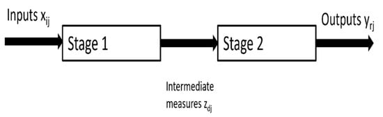
Figure 1.
Typical structure of a two-stage DEA model.
As can be observed, inputs enter stage 1 and produce the intermediate measures (which are considered the outputs of stage 1). Those intermediate measures are used as inputs for stage 2 of the process and produce the outputs. This structure of DMUs for DEA has proven very effective in increasing the robustness of efficiency measurements; however, as will become clearer in the next section, little attention has been paid to the weight distribution and weak discriminatory power of network models [30].
Consequently, the power of DEA as a monitoring tool for sustainability is diminished by the same issue that was identified in the beginning of this section: different people (policy makers, analysts, the public, etc.) have different values and perceptions of what sustainable development means and what should be used to measure sustainability. Thus, there is a need to increase the robustness of DEA by incorporating as many perceptions as possible in the measurement of sustainability without losing the value of its advantages.
To summarize, the following gaps have been identified: first, the employment of two-stage (or network) DEA models for sustainability assessments, despite its increasing use, has not reached the levels of use of classic, one-stage DEA models. Second, more efforts are necessary in order to increase the discriminatory power of two-stage models, and finally, research efforts need to be directed towards including more and diverse perceptions for the measurement of sustainability.
The purpose of the current paper is to address the above gaps by proposing a computational framework with a twofold functionality. First, it uses a two-stage Data Envelopment Analysis model with an alternative optimization metric that attempts to intervene in the weights of the inputs, intermediate measures and outputs to better reflect their importance for the DMUs. Second, the framework accompanies the DEA model with a computational stage that will attempt to incorporate different perceptions (meaning different combinations of inputs and outputs) and apply it in the measurement of sustainability of the EU 28 countries using machine learning techniques. To achieve this objective, the framework will rely on Exploratory Modeling and Analysis (EMA). EMA is a school of thought developed at RAND corporation [31] and promotes the exploratory use of quantitative methods despite methodological limitations, uncertainties and different perceptions. Employing an exploratory approach to sustainability measurement could reveal unanticipated implications of the initial assumptions regarding inputs and outputs. The use of computational experimentations to explore conjectures, models and datasets is not new. It has been applied in simulation models [5]), mathematics [32] and of course in various disciplines with the emergence of big data [33]. The approach requires computational power, development of new algorithms and techniques to analyze the data that will be generated.
Thus, EMA relies on Machine Learning (ML) techniques, even though validation of the developed models may not be possible. However, even when it is not possible to validate a model, exploration could lead to insights on how the different perceptions of sustainability give rise to unexpected results. Moreover, the use of computational explorations could facilitate the explanation of known facts and the discovery of commonalities among different perceptions of sustainability, hence leading towards the development of a composite definition of sustainable development.
For that reason, the combination of DEA and ML has been gaining traction in the literature. For example, Samoikenko and Osei-Bryson [34] combined DEA with clustering and Classification and Regression Trees (CART) to increase the discriminatory power of the method; Wu [35] integrated DEA with data mining and CART to evaluate the efficiency of Brazilian companies. De Nicola et al. [36] combined DEA with CART to evaluate the Italian health system. Nandy and Singh [37] used DEA to evaluate the efficiency of farms in India and employed machine learning to gain insights into which variables are crucial in predicting performance. Aydin and Yurdakul [38] separated countries in groups via clustering and then calculated the efficiency of how countries responded to COVID-19 in each cluster with DEA. Finally, Thaker et al. [39] employed DEA to evaluate the efficiency of Indian banks and then used Random Forest Regression to analyze the impact of corporate governance (and other bank characteristics) on the calculated efficiencies. Consequently, combining DEA with ML offers an alternative approach to the issue of inputs and outputs selection.
However, all the above combinations of DEA with ML are limited by the repeating theme of this introduction: that they do not consider different perceptions into the calculations. Furthermore, all the above attempts, in essence, worked towards reducing the size of the available data with the introduction of ML (e.g., using clustering). In the current paper, the opposite occurs; the variety of calculations under different perceptions can be seen as new data generators that are used as inputs for the ML stage of the model that add new layers of insights.
The novelties of the current paper are the following: first is the proposal and development of an alternative, two-stage DEA model with a different optimization metric and the proof of lemmas and a theorem. The second novelty is the integration of DEA with ML under an exploratory, multi-perspective (similar to a full factorial experimental design pattern) that will not only calculate the performance of EU countries in terms of sustainability, but at the same time will provide insights relevant to policy makers and the general public. Finally, several case studies are presented in the subsequent sections, and each can be considered an addition to the literature of DEA.
The rest of the paper is structured as follows: in Section 2, the issue of the weight flexibility in Data Envelopment Analysis is approached. The literature is reviewed, an alternative two-stage DEA model is proposed and it is applied in the calculation of the environmental performance of European countries. In Section 3, a new computational framework is proposed and applied in the calculation of the sustainability of European countries in a step-wise function. Conclusions, contributions of the current paper and future research avenues are explored in Section 4.
2. Weight Flexibility in Data Envelopment Analysis
2.1. Literature Review on Weights in Data Envelopment Analysis
Weighting flexibility has been met with some criticism, since a DMU’s efficiency assessment might be dominated by secondary activities, thus concealing inefficiencies of important factors in the Production Possibility Set [40], or might not reflect the preferences of the policy maker [41].
To solve these limitations, several approaches have been proposed. Sexton et al. [42] introduced the notion of cross efficiency, where each DMU is assessed in a peer evaluation mode with the optimal weights of all the other DMUs instead of its own [43]. However, Kao and Hung [44] argued that cross efficiency limits the information contained in the weights of the DMU’s inputs and outputs. The research on cross-efficiency evaluation has been very active in recent years, with papers attempting different approaches to establish appropriate weights [45] for both crisp and fuzzy data [46,47].
In another approach, several authors suggested modifications to the classic DEA models in order to obtain a Common Set of Weights on which the efficiency of all DMUs is calculated [48]. One stream of research in this approach is the use of virtual DMUs in the set that act as reference points for the real DMUs. Such virtual DMUs are hypothetical units that can act as a reference for the existing ones, either by assuming that they use inputs in the most economical ways to produce the maximum level of outputs (ideal DMUs), thus incentivizing the existing DMUs to imitate them, or by assuming that they use inputs in the most expensive way to produce the minimum level of outputs (anti-ideal DMUs), thus incentivizing the existing DMUs to deviate from the behavior as much as possible. Khalili-Damghani and Fadaei [49] used both an ideal and an anti-ideal DMU to increase the discrimination power of DEA. Finally, Azadi et al. [50] proposed models to calculate the efficiency of DMUs based on the distances to two virtual DMUs, considering both the pessimistic and optimistic approach of DEA.
Moreover, there are approaches to increase the discriminatory power of DEA by combining the classic model with another method. For example, Kritikos [51] combined DEA with TOPSIS in order to fully rank DMUs, while Simuany-Stern and Friedman [52] used the methodology with non-linear discriminant analysis. Another common approach is the combination of DEA with AHP; for example, in Thanassoulis et al. [53], the authors combined the two methods to evaluate higher education teaching performance. Moreover, DEA has been combined with Multi-Objective Linear Programming approaches (see for example [54,55,56]) that provide the Decision Maker with the opportunity to state their preferences through interventions in the weights. Finally, weight restrictions as part of the DEA model have been proposed as a solution to their flexibility in the literature. Weight restrictions can be seen as value judgments [57] that not only limit their flexibility, but also act positively on the discriminatory power of the model [58]. Examples of weight restriction methods include the work by Alirezaee and Afsharian [59] who used the trade-offs approach with an expanded Malmquist index to increase the discrimination of DMUs or the Cone-Ratio models [60] and Assurance Regions [61].
However, Jain et al. [41] point out that these weight restriction methods might also have some limitations such as increased subjectivity, since the models incorporate a priori information, lack of guarantee for feasibility or the assumption of a single policy maker. Even in cases where hybrid models are used for group decision-making contexts (for example, [62]) the final result relies on the assumption of compromise, which indicates a final (aggregate) Decision Maker. Moreover, all the approaches that were mentioned above are solutions for classic, one-stage Data Envelopment Analysis. For two-stage or Network DEA models, examples include the work by Mahdiloo et al. [30], who argued that little attention has been paid to the weight distribution and weak discriminatory power of network models. In their paper, they propose a multi-criteria DEA model, which is tested by assessing the sustainable design performances of car products. Gharakhami et al. [63] proposed a DEA variation that is based on goal programming, while Mavi et al. [64] used a similar approach to analyze the joint effects of eco-efficiency and eco-innovation. Halkos et al. [65] proposed a weight assurance region model to restrict the weights of the individual stages and applied the model to evaluate the efficiency of secondary education units of various countries. Finally, Kiaei and Matin [66] suggested a method based on separation vector to change a Multiple Objective problem into a single objective linear programming problem in two-stage DEA. Consequently, for two-stage DEA models, more efforts are necessary to address the limitations of weight distribution, especially when it comes to measuring the efficiency of complex processes such as sustainable development; in such cases, incorrect weight distribution might conceal inefficiencies of very important factors. For example, GHG emissions might not have equal importance compared to increased economic activity, despite the fact that they are crucial for the measurement of sustainability, thus providing an erroneous picture of sustainable development for the country/DMU under study. The present paper contributes to that aim.
2.2. Proposed Model
Assume a two-stage process for N DMUs. Each in the first stage uses inputs, the level of which is notated as , to produce intermediate measures, the level of which is notated as . The intermediate measures are used as inputs in the second stage to produce outputs, notated as
The efficiency of the first stage is calculated by the weighted sum of the intermediate measures over the weighted sum of the inputs, while the efficiency of the second stage is calculated by the weighted sum of the outputs over the weighted sum of the intermediate measures. The notations are used to represent the weights of the inputs, intermediate measures and outputs, respectively.
These are the typical problem statements and solution logic of two-stage DEA models, and several authors provided integrated models that attempted to simultaneously optimize the efficiencies of the two stages. Examples include: Liang et al. [67,68], Chen et al. [69,70], Kao and Hwang [71], Cook et al. [72] and Halkos et al. [73]. For indicative extensive reviews of two-stage and network DEA models, the reader is referred to the works of Castelli et al. [74], Halkos et al. [75], Kao [76] and Despotis et al. [77].
The two-stage model that is used by the authors Chen et al. [70] is presented below.
Subject to
The optimal value calculated by the model described in Equations (2)–(8) represents the overall efficiency of , a number between zero (inefficient) and one (efficient). Furthermore, the optimal values of the weights are used for the decomposition of the overall efficiency and the calculation of the efficiencies of the individual stages according to Equations [70]:
The values of are the optimal values of the weights of the inputs, intermediate measures, and outputs, respectively, that were calculated by Equations (2)–(8).
However, the above model searches for the best possible values of those variables in order to maximize the efficiency of . As a result, the weights retain the flexibility that was mentioned in the Introduction. The issue in two-stage DEA models has incentivized authors to overcome the weight flexibility limitation by proposing different extensions, such as in the works by Mahdiloo et al. [30] and Sun et al. [25].
The model that is developed in the context of the current paper is in the same direction as the papers of Mahdiloo et al. [30] and Sun et al. [25], and proposes an alternative extension to the model described by Equations (2)–(8) by actually introducing a different metric for the objective function using deviational variables:
Subject to
The main property of the model is the introduction of the variables . The variable represents the positive deviation and variable represents the negative deviation of the efficiency of stage 1 from reaching the maximum value. Variable represents the positive deviation while the variable represents the negative deviation of the efficiency of stage 2 from reaching its maximum value. Consequently, since in two-stage DEA it is assumed that the ratio of the sum of the weighed intermediate measures to the sum of the weighted inputs (stage 1) and the sum of weighted outputs to the sum of weighted intermediate measures should be smaller or equal to one (constraints (13), (15)), the introduction of the variables occurs in constraints (13) and (15) in order to make them equal to zero in the following manner:
Thus, the model represented by Equations (11)–(20) attempts to find the best possible values for , and by minimizing the deviations of both the first and second stage of the DEA model. By simultaneously minimizing the deviations of each stage (i.e., for stage 1 and for stage 2), the efficiencies of both stages are maximized at the same time and no priority is given for which stage should take precedence. Moreover, since we wish to attain the specific value of one for both stage efficiencies, both groups of deviational variables are included in the objective function to be minimized.
Equations (12) and (14) ensure that the efficiency scores of the first and second stage are smaller than one. Equations (13) and (15) indicate that the efficiency score for the first and second stage, respectively, when their respective deviations are added should be one, and to achieve that, it is assumed that (Equation (16)).
The efficiencies of the individual stages are calculated according to Equations (9) and (10), while the overall efficiency equals the average of the individual efficiencies, similar to the work by Mahdiloo et al. [30].
The contribution of the proposed model compared to the ones in the literature is the inclusion of both positive and negative deviational variables. The introduction of positive and negative deviations in such models is typical in the Multi-Criteria Decision Analysis literature, and although the model might work with fewer deviations, in the context of the current paper, the authors believe that although the inclusion of both positive and negative deviations adds a level of complexity to the model, it also offers a layer of rigor, which might increase the computational time but at the same time provides a more nuanced distribution of the weights without altering the core elements of the DEA methodology. In addition, the significance of each deviational variable in the objective function can be further fine-tuned, either within a level or between levels with appropriate weights, thus offering a trade-off vehicle of trading between the efficiencies.
The authors of the current paper recognize that the proposed alternative, two-stage DEA with a different optimization metric described by Equations (11)–(20) can be one of many approaches that use deviational variables; in order to examine whether the proposed approach was valid, three lemmas and one theorem were proved about the model described by Equations (11)–(20), which are presented in Appendix A. Finally, the proposed alternative approach to two-stage DEA might not offer a unique solution and one approach to mitigate the potential effects of that fact will be presented in Section 3 of the current paper.
2.3. Application
Another contribution of the current paper is the calculation of the environmental performance of European countries with the two-stage DEA model described by Equations (11)–(20). For the determination of the inputs, intermediate measures and outputs, the efforts of Tsaples and Papathanasiou [78] were used. The authors study the concept of sustainability and how DEA has tackled it and consider environmental performance as one of the dimensions of sustainability. Furthermore, Tsaples and Papathanasiou [79] use different combinations of inputs, intermediate measures and outputs to calculate the environmental performance of EU countries.
For the case study, the following measures are used:
- Inputs: Population, Gross electricity production [Thousand tons of oil equivalent (TOE)] ( in the DEA model)
- Intermediate measures: Final energy consumption [Terajoule] ( in the DEA model)
- Outputs: Terrestrial protected area (km2), Share of renewable energy in gross final energy consumption, Greenhouse gas emissions (in CO2 equivalent) ( in the DEA model)
The data source is Eurostat (https://ec.europa.eu/eurostat (accessed on 10 January 2021)) for the year 2018, which was the latest common year for which data were available for all countries during the writing of the current paper. The choice of the specific parameters was based on the works of Tsaples and Papathanasiou [78,79]. However, as the authors note in their literature review [24], despite the commonalities, the works in the literature use different sets of inputs and outputs to measure sustainability. For example, the input Population can be found in papers such as the one by Lo Storto [80], while the pollution outputs can be found in several papers, such as the one by Li et al. [81]. Nonetheless, as it was stated in the Introduction, the objective of the current paper is to propose a computational framework that will incorporate all those different perceptions (hence different combinations of parameters) into a single measure of sustainability.
Finally, the output Greenhouse gas emissions is considered undesirable, which contradicts the nature of outputs in Data Envelopment Analysis, which should always be maximized. Thus, the undesirable output of the case study is rendered into a “desirable” one with a linear monotonic transformation [82].
Table 1 below illustrates the results obtained from the alternative metric two-stage DEA and the corresponding results obtained from the model of Chen et al. [70].

Table 1.
Results from the proposed, alternative metric two-stage DEA and the ones obtained by the models of Chen et al. [70].
The column named E0 indicates the overall environmental performance of the country, E1 indicates the performance of the first stage and E2 indicates the performance of the second stage. The first aspect to observe is that the results of the individual stages for the proposed alternative are almost similar to the ones calculated with the model of Chen et al. [70], nonetheless with notable differences. These differences, we argue, are the result of the introduction of the deviational variables that, apart from restricting the values of the optimal weights, essentially induce the optimization of a different metric in the objective function and the following calculation of the overall efficiency by the arithmetic mean of the individual efficiencies. Furthermore, the two models differ in the average overall efficiency, which is larger in the proposed variation and the range of the values of the overall efficiency, which, in the proposed model, is smaller than that of Chen et al. [70]. Notably, the model of Chen et al. [70] assumes that the overall efficiency is derived as the product of the divisional efficiency scores, whereas in the proposed model, the overall efficiency is calculated as the weighted average of the divisional efficiency scores. Therefore, it is true that comparing the overall efficiency scores would not make much sense. It is worth mentioning, though, that the overall efficiency in the proposed model is defined through a compensatory approach, whereas the model of Chen et al. [70] employs a non-compensatory approach. Consequently, it is mathematically expected that the proposed model would certainly be allowed to attain higher (or equal) overall efficiency scores. In Table 1, as both models estimate almost identical divisional efficiency scores, they will also provide almost the same overall efficiency scores under any common definition of the overall efficiency.
The accumulated small differences result in different rankings of the countries according to their overall efficiency. Countries that seemed to perform better under the variation of Chen et al. [70], such as Poland, Portugal and Greece, move down the ranking in the proposed variation of the current paper. Finally, we observe that despite the above notable observations, the values of the efficiencies of the individual stages do not differ much, and the fact that the countries that are in the efficient frontiers of the first and the second stages, respectively, remain the same under both variations increases the confidence in the results. In combination with the results from the paper of Mahdiloo et al. [30], where the authors observed similar behavior when they compared their model with that of Chen et al. [70], the robustness of both the results and the models increases.
To get a better understanding of how the alternative variation compares to that of Chen et al. [70], an additional illustration was performed by adding: to the inputs the Gross fixed capital at current prices (PPS) and the Total Labor force (×1000 persons), to the intermediate measures the Domestic material consumption [Thousand tons] and to the outputs the Total expenditure [Euro per inhabitant]. The results are tabulated in Table 2 below.
Table 2.
Another set of results from the two variations with additional parameters.
The inclusion of more parameters in the two-stage models alters the results, which is not unexpected. However, the conclusions from the previous table also hold for the results in Table 2. Nonetheless, the differences in the overall efficiency between the proposed method and that of Chen et al. [70] are larger.
In conclusion, the proposed DEA variation with the alternative optimization metric does not come without limitations. Firstly, the calculated solution might not be unique. Furthermore, in its current version, the proposed model uses a compensatory approach to calculate the overall efficiency from the stage ones, which might not be applicable in all contexts.
Despite the limitations, the alternative model that is proposed in the current paper is accompanied by several advantages, as follows: (1) the introduction of both negative and positive deviational variables distinguishes the proposed model from that of Chen et al. [70] (and the model by Mahdiloo et al. [30]) in a qualitative manner: the deviational variables in the first stage push the stage efficiency to increase, to the detriment of the efficiency of the second stage. (2) At the same time, the deviational variables of the second stage push the stage efficiency to increase in detriment to the efficiency of the first stage. Hence, a trade-off occurs between the two stage efficiencies that ultimately drives the overall efficiency upwards. (3) The model provides a more nuanced distribution of the weights without altering the core elements of the DEA methodology. (4) In addition, the significance of each deviational variable in the objective function can be further fine-tuned, either within a level or between levels with appropriate weights, thus offering a trade-off vehicle between the efficiencies and a scheme to incorporate the preferences of decision makers.
3. Exploratory, Multi-Dimensional Data Envelopment Analysis
As was mentioned above, environmental performance is considered only one of the three (or more) dimensions of sustainability. Consequently, moving in the direction of adding more dimensions to measure sustainability, the need arises to move from a two-stage DEA model to a multi-level or multi-dimensional model that will allow the incorporation of these dimensions without succumbing to the methodological limitations of DEA. In the following sub-sections, a new framework is proposed for the incorporation of multiple dimensions.
3.1. Multi-Dimensional DEA for the Construction of Composite Indicators
The typical calculation of sustainability involves three dimensions: economic, environmental and social. Thus, the calculation of the environmental performance in the previous section can be considered as part of sustainability, despite the fact that many of the inputs, intermediate measures and outputs that have been used by the various authors resemble those that are used in the DEA literature for the calculation of sustainability.
However, for a more inclusive calculation of sustainability that is not limited by the number of inputs and outputs that can be used, the proposed alternative, two-stage model that was described by Equations (11)–(20) can be incorporated in the framework proposed by Tsaples and Papathanasiou [79] and shown in Figure 2.
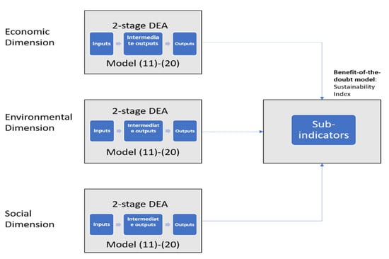
Figure 2.
Framework for the construction of composite indicators proposed by Tsaples and Papathanasiou [79].
Each sub-indicator/dimension is calculated using Equations (11)–(20) and the overall performance of each sub-indicator/dimension is used in a Benefit-of-the-Doubt (BoD) model to calculate the overall sustainability index. The BoD model is described by Equations (23)–(25) below [83]:
Subject to:
The BoD model described by Equations (23)–(25) is a typical DEA model with the inputs designated as one. As a result, the model calculates the optimal weights allowing maximum flexibility. In contrast with the proposed two-stage alternative of Equations (11)–(20), the BoD model does not include any restrictions to the weights because the dimensions that are included are typical of sustainability (despite the differences in the underlying measures that are used to calculate those indicators) and limited in number. Moreover, the simplicity of the BoD model, the opportunities that it allows to account for different (countries’) backgrounds [84], the fact that it has been used by numerous studies (see [85] for an inclusive account) and has been proposed by OECD for the construction of composite indicators [86] mean that it can be used without any intervention in the weights. As mentioned in the above paper, its main advantage is that “it results in idiosyncratic weights to aggregate sub-indicators that vary both across sub-indicators and evaluated decision-making units (DMUs)”. In other words, “each evaluated DMU is allowed to choose a set of weights that maximizes its performance in terms of the resulting value of the composite indicator under the restriction that if the same set of weights is used by any other evaluated DMU it will not result in a value of the composite indicator that is greater than one” [85] (p. 1). The use of a BoD model is not unique and alternative methods can be used equally successfully and efficiently (for example, Shannon’s entropy in the example [87]). However, in the context of the current paper, the BoD approach is preferred because the overall proposed model continues to be two-stage DEA, in which the first stage consists of two-stage DEA models that calculate the (more refined) dimensions that will be used in the BoD model that brings the above desired properties for the construction of a final scalar index for each country. Thus, the framework is characterized by an esoteric, elegant consistency.
In the current paper, the following are used for each dimension:
- Economic
- -
- Inputs: Gross fixed capital at current prices (PPS); Total Labor force (×1000 persons);
- -
- Intermediate measures: GDP per capita in PPS Index (EU28 = 100);
- -
- Outputs: Median equivalized net income [Purchasing power standard (PPS)]; Final consumption expenditure of households [Current prices, million euro].
- Environmental
- -
- Inputs: Population, Gross electricity production [Thousand tons of oil equivalent (TOE)];
- -
- Intermediate measures: Final energy consumption (Terajoule);
- -
- Outputs: Terrestrial protected area (km2), Share of renewable energy in gross final energy consumption (%), Greenhouse gas emissions (in CO2 equivalent).
- Social
- -
- Inputs: Gross fixed capital at current prices (PPS), GDP per capita in PPS Index (EU28 = 100);
- -
- Intermediate measures: Total expenditure (Euro per inhabitant);
- -
- Outputs: Patent applications to the European patent office (EPO) by priority year; Overall life satisfaction; Satisfaction with living environment; Percentage of females in total labor population [79].
As it can be observed in Table 3, there are four countries that are considered sustainable compared to the rest of the set: Germany, Estonia, Latvia and Malta. The rest of the countries can be grouped into two broad categories: those that have a sustainability index above 0.7 compared to the other countries and those that have a sustainability index below 0.7., which includes Belgium, Czech Republic, Ireland, Greece, Spain, Hungary, Netherlands, Portugal and Slovakia. Furthermore, the Spearman Correlation Coefficient was calculated for:
Table 3.
Results for the construction of a sustainability composite indicator.
- Sustainability–Economic sub-indicator: 0.635
- Sustainability–Environmental sub-indicator: 0.627
- Sustainability–Social sub-indicator: 0.616
The coefficients illustrate that the sustainability of each country depends almost equally on each sub-indicator, with the economic-sub-indicator, however, having a slightly larger coefficient.
3.2. Proposed DEA-ML Computational Framework
Nonetheless, the above calculated sustainability index suffers from the same limitations that were identified in the Introduction and in the previous section: Since there is no unique, “correct” definition of sustainability, the same indicator can be calculated by using different variations of DEA and/or different combinations of inputs, intermediate measures and outputs.
Furthermore, the proposed two-stage DEA variation might not offer a unique solution that could alter the final results of the calculated index. Finally, one could argue that the BoD model that was used to aggregate the individual dimensions into one sustainability index does not pose any restrictions to the weights, similar to those proposed in the initial two-stage DEA model. Thus, methodological limitations might limit the value of the final results.
Consequently, there is the need to have an indicator of sustainability that will incorporate all these different perceptions that may arise—where perceptions mean different DEA and BoD variations and/or different combinations of inputs, intermediate measures and outputs—and at the same time limit the impact of methodological limitations. Such an indicator would be useful in policy design (and policy making in general) because, as Foster and Sen [88] proposed, uniqueness is not a prerequisite to make agreed judgments. Hence, the proposed computational framework is based on this principle, and it consists of the following steps:
Step 1: Define different perceptions of sustainability and for each perception:
- (a)
- Define how many sub-indicators will be entailed in this perception’s sustainability index;
- (b)
- Define the inputs, intermediate measures and outputs that each sub-indicator will entail;
- (c)
- Repeat for all perceptions.
Step 2: Define the variation of DEA that will calculate the value of the sub-indicators.
- (a)
- Calculate the sub-indicators;
- (b)
- Calculate the perception’s sustainability index using model (23)–(25);
- (c)
- Once all sustainability indices for all perceptions are calculated, calculate the mean value for each country/DMU.
Step 3: Use machine learning to gain insights into the sustainability of each country under different perceptions.
Figure 3 below illustrates the proposed computational framework.
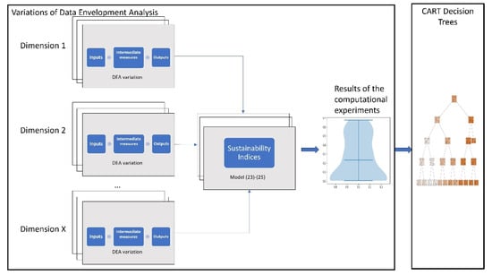
Figure 3.
Exploratory, multi-dimensional data envelopment analysis.
Consequently, by blending DEA with ML, the available data and analyses are expanded, which contributes to investigating the topic under study (thus implicitly adding new layers to the initial problem), meaning that greater insights are revealed. Furthermore, the absence of a unique solution created by the proposed alternative two-stage model of Equations (11)–(20) can be considered a methodological limitation; however, the issue becomes not of central importance per se, since in the context of the current paper, the model will be used repeatedly and with different data to generate different results, in accordance with the philosophy of Exploratory Modeling and Analysis, where methodological limitations lose their impact from the generation of numerous results under different assumptions. Hence, the exploratory framework offers not only a slight deviation from the typical way that DEA is used, but also a complementary research avenue on the issues of interpretability and transparency of algorithms and/or quantitative methods: by blending methodologies under a multi-perspective design, algorithms become more inclusive and democratic (in the sense that the Benefit-of-the-Doubt notion inherent in the aforementioned DEA formulations is further enriched). Hence, decision support can take a step towards the generation of collective knowledge that includes different values, perceptions and dimensions.
3.3. Illustration of the Proposed DEA-ML Computational Framework
Step 1: In the context of the current paper, three types of Economic (with measures including, for example, Total Labor Force, Gross Fixed Capital at current prices as inputs, GDP per capita as intermediate measures and Median equivalized net income and Final consumption expenditure of households as outputs), three types of Environmental (with measures including, for example, Gross Electricity Consumption as inputs, Energy Consumption as intermediate measures and Greenhouse Gas Emissions as outputs), three types of Social (with measures including, for example, Overall life satisfaction, percentage of females in total labor population as outputs) and two types of Research and Development (R&D) (with measures including, for example, Intramural R&D expenditures, Patent applications to the EPO as outputs) dimensions are defined. These 11 different types of dimensions are combined in all the possible combinations of three and four dimensions, resulting in 135 different perceptions of sustainability. Consequently, in the context of the current paper, the choice of parameters for the models becomes secondary in importance, with the purposing of reducing the bias of the analyst or decision maker and the methodological limitations of DEA. All the parameters/variables that are used in the calculations along with summary statistics are presented in Appendix B.
Step 2: Each of these 135 perceptions are used with the proposed DEA model that is described by Equations (11)–(20) and (23)–(25). The mean sustainability of the countries with the proposed DEA variation is displayed in Table 4 below:
Table 4.
Mean sustainability calculated with the proposed DEA model (Equations (11)–(20) and (23)–(25)).
Hence, the inclusion of different perceptions alters the results that were illustrated in Table 3. Under multiple perceptions, Malta, Latvia and Luxemburg have the highest sustainability compared to the rest of the countries. Moreover, with all the different variations of sub-indicators, there are countries for which the mean sustainability falls below 0.5, such as the Czech Republic, Ireland, Italy and the Netherlands. Finally, there are no countries for which the mean sustainability increased with the inclusion of different parameters; only Malta managed to keep the sustainability at the value of one in both cases.
Figure 4 below illustrates the results of the 135 calculations of sustainability on violin plots.
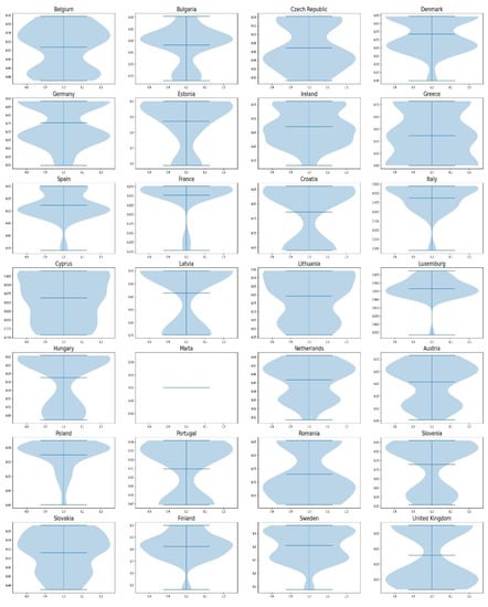
Figure 4.
Violin plots of the sustainability of 135 different perceptions calculated with the proposed, alternative metric two-stage DEA.
The y axis indicates the measurement of sustainability, while the x axis indicates the distribution of the sustainability indices that were calculated; wider sections of the density indicate that there is a higher probability that data points will take the given value, while narrow sections indicate lower probability.
The first aspect to observe is that Latvia concentrates the majority of their values on the upper side of the violin plot, while Malta has a constant value of one for all calculations, indicating that compared to the rest, the two countries have a high sustainability no matter the perception; thus, the robustness of the conclusion increases. For the rest of the countries, the different perceptions create different situations for their sustainability. For example, Greece has a mean sustainability of 0.57; however, its values can change depending to the perception from 0.45 to 0.75, with the majority of the values concentrated between 0.5 and 0.6. Thus, the sustainability of Greece changes with different perceptions in a significant way, weakening the declaration of any robust conclusions.
Apart from the calculation of the sustainability indices under different perceptions with the proposed two-stage DEA, Step 2 of the computational framework includes the use of different variations of DEA. In the present application, the classic two-stage model of Chen et al. [70], and an adaptation of the Constant Returns to Scale (CRS) DEA [16] and of the Variable Returns to Scale (VRS) [17] are used (along with the proposed variation). For the last two DEA variations, the classic DEA models are used in a chained way to accommodate the two-stage nature of the models. More specifically, each combination of inputs, intermediate measures and outputs is used in the chained way of the classic one-stage models as follows: the efficiency of the first stage is calculated with the inputs and the intermediate measures as outputs, using either CRS or VRS DEA. The efficiency of the second stage is calculated with the intermediate measures as inputs and the outputs, using (similar to the first stage) either CRS or VRS DEA. The sustainability index is calculated by multiplying the efficiencies of the two stages. Finally, the sustainability index of each perception is calculated using the BoD model [83] (Table 5).
Table 5.
Mean sustainability calculated with all DEA variations.
The inclusion of different variations of DEA (which can be chosen by the analyst and/or the policy maker) with different combinations of inputs and outputs increases the robustness of the results, since many sustainability indices will be calculated that can capture different perceptions both methodologically (which method is the more “correct”) and context wise (which combination of inputs, outputs and intermediates is the more “correct”).
As can be observed in Table 5, the mean sustainability changes again, indicating that the methodological framework that is used matters in the calculation of the final index. In the current illustration, there are countries where the mean sustainability increases with the inclusion of other DEA variations (such as Belgium, Luxemburg and the Netherlands), others where it is almost the same (such as Malta) and those for which the mean sustainability decreases (the rest of the countries). Moreover, the Spearman correlation coefficient for the two mean sustainability indices of Table 4 and Table 5 was calculated and found to be equal to 0.752, which indicates a strong positive correlation between the two indices.
These changes are also mirrored in the violin plots of the sustainability, displayed on Figure 5.
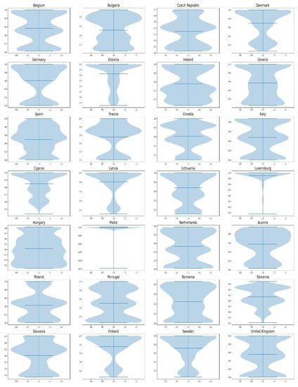
Figure 5.
Violin plots of the sustainability of 135 different perceptions calculated with all DEA variations.
Focusing again on the example of Greece, there are combinations of sub-indicators and DEA variations that produce high sustainability indices. Furthermore, the number of values below the mean increases with all DEA variations.
Step 3: The final step of the proposed computational framework is to use machine learning techniques in the results of the above computations with the purpose of revealing insights into how the sustainability of countries behaves under different perceptions. For the current paper, the Classification and Regression Decision Trees (CART) are used; since they are not computationally costly, they can be used as tools to communicate with non-experts and offer deep interpretational capabilities [89]. Consequently, the use of Machine Learning assists in identifying those features that affect the calculations of sustainability under different perceptions and methodological frameworks. However, CART trees tend to overfit the data to their training set and are considered weak learners [90], and for that reason, an additional ML technique will be used: boosting regression [91]. Boosting regression is considered a slow learner, where each tree is generated using information from previous ones [92]. Moreover, the technique will also reveal the relative influence of the individual sub-indicator to the index of sustainability, which could provide further insights into the analysis of the results. It is more robust than CART trees, but this robustness comes at the detriment of intuitive communication capabilities that are the main characteristic of CART trees. Consequently, the use of the two Machine Learning techniques will limit the methodological weaknesses of each method, while providing results and insights that are robust and independent of the technique used. Following the logic of the previous steps, the focus will be on Greece. Figure 6 below illustrates the CART tree of Greece, along with the relative influence of the sub-indicators that were used in all perceptions.
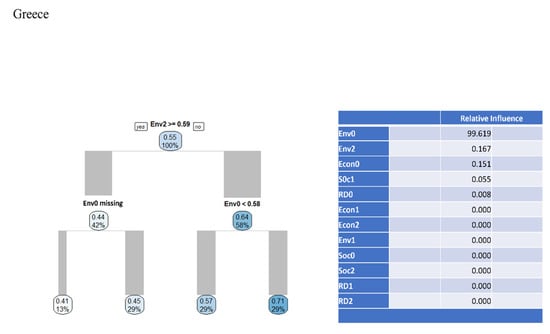
Figure 6.
CART trees for Greece under the proposed, alternative metric two-stage DEA.
As can be observed, the overall environmental performance is the sub-indicator that influences the overall sustainability the most. Furthermore, the CART tree illustrates that when the environmental performance of the second stage is larger than 0.59 and the overall environmental performance is missing, the sustainability of Greece takes its lowest values, further supporting the importance of the sub-indicator.
The final part of the analysis is to perform data mining on the countries when all DEA variations are used. For Greece (Figure 7), the most important sub-indicators become those of the overall economic one and the one representing research and development. From the CART tree, if the overall economic performance is lower than 0.045 and the overall research and development index is lower than 0.59, the sustainability of Greece (under all DEA variations) has its lowest values.
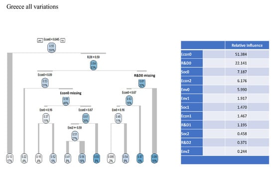
Figure 7.
CART trees for Greece under all DEA variations.
4. Conclusions
The purpose of this paper was to propose a computational framework with a twofold contribution: at its initial phase, it uses a two-stage Data Envelopment Analysis model with an alternative optimization metric that attempts to intervene on the weights of the inputs, intermediate measures and outputs to better reflect their importance for the DMUs. The model takes advantage of deviational variables to handle the variations attributed to the weights distribution. The deviational variables provide a vehicle of interventions on the weights distribution through the goal programming formulation inherent to DEA. The model was used to calculate the environmental performance of EU countries and a comparison was provided with the two-stage variations of Chen et al. [70]. The results illustrate that the two variations share similarities but also notable differences for environmental performances, and obviously there are changes in the rankings. This is attributed to the fact that the alternative DEA variation uses a different optimization metric through the additional variables that impose limitations on the distributions of the calculated weights.
The second area of contribution of the framework is the integration of a computational stage, which attempts to incorporate different perceptions (that is, different combinations of inputs and outputs) and apply it in the measurement of sustainability of the EU 28 countries using machine learning techniques. This is extremely useful and important especially in the case of multi-dimensional constructs such as sustainability. The overall computational stage relies on the use of multi-level Data Envelopment Analysis in combination with classic DEA variations and on the application of these models for different combinations of inputs, intermediate measures and outputs that represent different perceptions of what sustainability is. Finally, the exploratory analysis on the outcomes with the use of Machine Learning methodologies such as CART decision trees concludes the computational part of the paper by proposing sustainability paths according to each country’s strengths and weaknesses as it is further summarized in the following paragraph.
In this direction, it is worth pointing out that this framework follows the school of thought of Exploratory Modeling and Analysis that supports the use of models and quantitative methods in an exploratory way, not to predict or monitor policy cycles accurately (which can be considered impossible) but to gain insights by incorporating different perceptions and methodological approaches towards the same problem, thus increasing the robustness of the results [93]. In the current paper, we applied this approach in the measurement of sustainability of EU 28 countries. Concretely, the computational experiments illustrated that the different perceptions of how sustainability is measured, and the use of different DEA variations (hence different methodological frameworks) affect the final results.
Finally, the blend of DEA with machine learning (applied on the results of DEA for the various scenarios) revealed insights on the areas to which policy makers could direct investments to increase sustainability. In addition, the ML application contributed to the identification of the most important features of sustainability for the various countries, something that could have direct implications in the area of EU policy-making: for example, countries that share similar features that drive the behavior of sustainability could be grouped together in clusters and policies, laws, regulations, etc., could be adapted to those clusters in order to boost the particular features that would increase their sustainability. As a result, policy making has the potential to become customized (adapted to the specifics of each group) without missing its overall and principal theme of pursuing sustainable development. This adaptive and adaptable policy-making could be of great assistance, especially when new countries are negotiating their entry to the Union; based on the features that affect the sustainability of the new countries, they could follow the regulations and laws of the appropriate cluster. Finally, the inclusion of new layers and perceptions renders the algorithms more inclusive and participatory, increasing their transparency, thus improving the trust in the final results.
However, the proposed framework is not without limitations. Regarding the definition and/or methodological framework for sustainability, a new approach could be taken: a bottom-up approach, where scientists propose a unified methodological and/or computational framework that attempts to mitigate the limitations of individual methods and integrates different and diverse definitions of sustainability into the same measurement.
Moreover, the addition of this new layer means that the process becomes more computationally costly and new conceptual questions arise; for example, when is it valid to break the inner loop, stop adding new perceptions and report the conclusions? How many new perceptions are necessary to get a clearer picture? Finally, the proposed methodological framework relies on an intrinsic assumption that the majority of perceptions drives the measure of sustainability towards its “real value”. However, this is not always the case, since the notion of sustainability constantly evolves, meaning that perceptions that currently represent the minority in the calculations could become more prevalent in the future. Hence, the proposed computational framework could be enriched further with notions and algorithms that represent values more clearly. Of course, such an inclusion is not limited to the current framework but is a problem that is central to the overall research of the Artificial Intelligence community.
Such questions will drive future research efforts of the current study. Further directions of research include the development of a user interface that could be used by non-experts, and the inclusion of supplementary variations of DEA (for example, the VRS variation of the proposed two-stage model described by Equations (11)–(20), or a version of the BoD model with weight restrictions), the generation of additional sub-indicators along with various data sources. Finally, the framework could be enriched with methods other than DEA which would allow the Machine Learning techniques to identify not only the differences in the context (sub-indicators) but also in the method that was used.
Author Contributions
Conceptualization, G.T., J.P. and A.C.G.; Formal analysis, G.T., J.P. and A.C.G.; Investigation, G.T., J.P. and A.C.G.; Methodology, G.T., J.P. and A.C.G.; Writing—original draft, G.T.; Writing—review & editing, J.P. and A.C.G. All authors have read and agreed to the published version of the manuscript.
Funding
This research received no external funding.
Data Availability Statement
Data are available upon request.
Conflicts of Interest
The authors declare no conflict of interest.
Appendix A
The following lemmas and theorem about the model described by Equations (11)–(20) are proved based on the work by Sun et al. [25] and Khalili-Damghani and Fadaei [45].
Lemma 1.
The constraints of the model described by Equations (11)–(20) form a non-empty, convex set.
Proof of Lemma 1.
The constraints (11)–(20) constitute a non-empty set named . If , then Hence, is a convex set. □
Lemma 2.
The objective function (11) is convex in the defined domain.
Proof of Lemma 2.
The Hessian matrix of the objective function is:
The matrix is always zero; thus, objective function (11) is a strictly convex function. □
Lemma 3.
The model described by Equations (11)–(20) is always feasible.
Proof of Lemma 3.
Suppose that an arbitrary solution of the model of the form:
Substituting Equations (A1) and (A2) in Equation (12): .
Substituting Equations (A1), (A2), (A4) and (A6) in Equation (13): .
Substituting Equations (A2) and (A3) in Equation (14): .
Substituting Equations (A2), (A3), (A5) and (A7) in Equation (15): .
Finally, substituting Equation (A2) in Equation (16): .
All constraints are satisfied with the arbitrary solution; thus, the model (11)–(20) is feasible. □
Theorem 1.
The model described by Equations (11)–(20) has an optimal solution.
Proof of Theorem 1.
is a non-empty, convex set (Lemma 1); the objective function is strictly convex (Lemma 2) and the model has a feasible solution (Lemma 3). Consequently, the solution obtained by the model is optimal. □
Appendix B
The choice of the parameters that were used to form the various sub-indicators was based on the literature (from works such as [9,24,73,78,79,80,81,94,95]) and the availability of common data. The authors do not claim that the list is exhaustive, but it serves to illustrate the capabilities of the proposed computational framework. Table A1 below summarizes the parameters, along with the major descriptive statistics of the data.
Table A1.
Parameters that are used in the compuational framework and summary statistics.
Table A1.
Parameters that are used in the compuational framework and summary statistics.
| Gross Fixed Capital at Current Prices (PPS) | Total Labor Force (×1000 Persons) | GDP per Capita in PPS Index (EU28 = 100) | Median Equivalised Net Income [Purchasing Power Standard (PPS)]—2018 | Final Consumption Expenditure of Households [Current Prices, Million Euro] | Population—2018 | |
|---|---|---|---|---|---|---|
| Mean | 93.7035714 | 8954.214286 | 97.60714286 | 15,896.46429 | 309,080.5929 | 17,970,379.21 |
| Standard Error | 25.2418411 | 2219.976821 | 7.815724769 | 1144.509393 | 89,744.88872 | 4,373,182.198 |
| Median | 35.85 | 4360.45 | 84.5 | 16372.5 | 122,017.75 | 8,846,162.5 |
| Standard Deviation | 133.567268 | 11,747.01317 | 41.35692811 | 6056.174452 | 474,885.314 | 23,140,705.07 |
| Sample Variance | 17,840.2152 | 137,992,318.5 | 1710.395503 | 36,677,249 | 2.25516 × 10¹¹ | 5.35492 × 10¹⁴ |
| Kurtosis | 4.02051893 | 2.281925743 | 8.29166899 | 0.182552646 | 2.792124589 | 1.428904095 |
| Skewness | 2.11001276 | 1.770197969 | 2.325043795 | 0.448817209 | 1.981594431 | 1.622982 |
| Range | 526.2 | 44,245.7 | 215 | 25,880 | 1,664,272.9 | 81,388,230 |
| Minimum | 1.7 | 193.3 | 46 | 6278 | 6506.1 | 414,027 |
| Maximum | 527.9 | 44,439 | 261 | 32,158 | 1,670,779 | 81,802,257 |
| Gross electricity production [Thousand tonnes of oil equivalent (TOE)]—2018 | Domestic material consumption [Thousand tonnes]—2018 | Final energy consumption [Terajoule] —2018 | Terrestrial protected area (km2)—2018 | Share of renewable energy in gross final energy consumption | Greenhouse gas emissions (in CO2 equivalent) | |
| Mean | 10,048.5454 | 246,185.8875 | 424,169.6536 | 28,009 | 18.53214286 | 9.228571429 |
| Standard Error | 2697.45258 | 54,633.58413 | 110,868.6098 | 5782.166667 | 2.211867065 | 0.624962584 |
| Median | 4853.78 | 148,400.71 | 214,985.875 | 16,821.5 | 15.75 | 8.4 |
| Standard Deviation | 14,273.5774 | 289,093.7537 | 586,661.5397 | 30,596.35008 | 11.70410038 | 3.306991152 |
| Sample Variance | 203,735,012 | 83,575,198,424 | 3.44172 × 10¹¹ | 936,136,638.3 | 136.9859656 | 10.93619048 |
| Kurtosis | 4.39672619 | 4.383577372 | 3.565649211 | 4.921733029 | 0.957448781 | 3.456735643 |
| Skewness | 2.17413267 | 2.014708432 | 2.041196627 | 1.92448185 | 0.958061175 | 1.586879483 |
| Range | 54,998.36 | 1,239,884.92 | 2,309,837.03 | 137,974 | 48.5 | 14.9 |
| Minimum | 168.71 | 6499.1 | 3892.59 | 42 | 3.5 | 5.4 |
| Maximum | 55,167.07 | 1,246,384.02 | 2,313,729.62 | 138,016 | 52 | 20.3 |
| Total expenditure [Euro per inhabitant] | Mean consumption expenditure of private households on cultural goods and services by COICOP consumption purpose [Purchasing power standard (PPS)] | Patent applications to the European patent office (EPO) by priority year | Overall life satisfaction | Satisfaction with living environment | Percentage of females in total labor population—2018 | |
| Mean | 7182.62071 | 25,608.67857 | 1951.743214 | 6.971428571 | 7.221428571 | 68.53214286 |
| Standard Error | 993.301805 | 1686.520727 | 746.3961868 | 0.135581946 | 0.148480589 | 1.349613442 |
| Median | 4696.11 | 26,815 | 277.075 | 7.05 | 7.55 | 68.6 |
| Standard Deviation | 5256.0591 | 8924.228852 | 3949.55738 | 0.717432223 | 0.785685425 | 7.141483069 |
| Sample Variance | 27,626,157.3 | 79,641,860.6 | 15,599,003.5 | 0.514708995 | 0.617301587 | 51.00078042 |
| Kurtosis | −0.1173526 | 0.381582258 | 12.94505502 | 1.597491057 | 0.06125311 | 1.020390146 |
| Skewness | 0.82586947 | 0.374300212 | 3.389370605 | −0.877951855 | −0.844073462 | −0.959481566 |
| Range | 19,595.89 | 38,416 | 18,875.07 | 3.2 | 3.2 | 31.1 |
| Minimum | 1248.76 | 11,422 | 6.63 | 4.8 | 5.2 | 49.1 |
| Maximum | 20,844.65 | 49,838 | 18,881.7 | 8 | 8.4 | 80.2 |
| Satisfaction with financial situation | Intramural R&D expenditure (GERD) by sectors of performance [Euro per inhabitant] | Pupils and students enrolled All ISCED 2011 levels excluding early childhood educational development | Participation rate in education and training (last 4 weeks) by sex and age. From 25 to 64 years. Percentage | Life expectancy at birth | Urban population exposure to air pollution by particulate matter [Particulates < 2.5µm] | |
| Mean | 5.90714286 | 488.85 | 3,872,286.429 | 11.56785714 | 80.225 | 13.275 |
| Standard Error | 0.19134228 | 86.49583843 | 942,453.4172 | 1.463814449 | 0.523864986 | 1.018423216 |
| Median | 5.8 | 281.75 | 1,792,249 | 9.4 | 81.5 | 12.95 |
| Standard Deviation | 1.01248816 | 457.6929559 | 4,986,994.728 | 7.745777993 | 2.772032948 | 5.388989117 |
| Sample Variance | 1.02513228 | 209,482.8419 | 2.48701 × 10¹³ | 59.99707672 | 7.684166667 | 29.0412037 |
| Kurtosis | −0.3674502 | −0.514620128 | 1.455757741 | 0.550769838 | −0.864099668 | 0.149557265 |
| Skewness | −0.0743634 | 0.888998451 | 1.644603126 | 1.007501236 | −0.778315177 | −0.212994905 |
| Range | 3.9 | 1479.7 | 16,110,645 | 30.5 | 8.5 | 24.3 |
| Minimum | 3.7 | 27.9 | 82,343 | 0.9 | 75 | 0 |
| Maximum | 7.6 | 1507.6 | 16,192,988 | 31.4 | 83.5 | 24.3 |
| Carbon dioxide [thousand tonnes] | People at risk of poverty or social exclusion [thousand persons] | Final energy consumption [Million tonnes of oil equivalent (TOE)] | ||||
| Mean | 112,130.516 | 3924 | 40.14642857 | |||
| Standard Error | 30,703.5494 | 967.6611291 | 10.04674016 | |||
| Median | 43,570.865 | 1667 | 17.725 | |||
| Standard Deviation | 162,467.912 | 5120.381402 | 53.16235191 | |||
| Sample Variance | 2.6396E × 10 | 26,218,305.7 | 2826.235661 | |||
| Kurtosis | 6.71719926 | 1.04478003 | 3.634446153 | |||
| Skewness | 2.39557289 | 1.556049423 | 1.987717623 | |||
| Range | 728,021.85 | 16,352 | 214.71 | |||
| Minimum | −1974.29 | 89 | 0.66 | |||
| Maximum | 726,047.56 | 16,441 | 215.37 |
References
- Tsoukias, A.; Montibeller, G.; Lucertini, G.; Belton, V. Policy Analytics: An Agenda for Research and Practice. EURO J. Decis. Process. 2013, 1, 115–134. [Google Scholar] [CrossRef]
- Bankes, S. Exploratory Modeling for Policy Analysis. Oper. Res. 1993, 41, 435–449. [Google Scholar] [CrossRef]
- Moraffah, R.; Karami, M.; Guo, R.; Raglin, A.; Liu, H. Causal Interpretability for Machine Learning-Problems, Methods and Evaluation. ACM SIGKDD Explor. Newsl. 2020, 22, 18–33. [Google Scholar] [CrossRef]
- Lewis, M.; Li, H.; Sycara, K. Deep Learning, Transparency, and Trust in Human Robot Teamwork. In Trust in Human-Robot Interaction; Elsevier: Amsterdam, The Netherlands, 2021; pp. 321–352. [Google Scholar]
- Kwakkel, J.H.; Pruyt, E. Exploratory Modeling and Analysis, an Approach for Model-Based Foresight under Deep Uncertainty. Technol. Forecast. Soc. Chang. 2013, 80, 419–431. [Google Scholar] [CrossRef]
- Brundtland, G.H.; Khalid, M.; Agnelli, S.; Al-Athel, S.; Chidzero, B. Our Common Future; Oxford University Press: Oxford, NY, USA, 1987; p. 8. [Google Scholar]
- Robinson, J. Squaring the Circle? Some Thoughts on the Idea of Sustainable Development. Ecol. Econ. 2004, 48, 369–384. [Google Scholar] [CrossRef]
- Santana, N.B.; Mariano, E.B.; Camioto, F.d.C.; Rebelatto, D.A.d.N. National Innovative Capacity as Determinant in Sustainable Development: A Comparison between the BRICS and G7 Countries. Int. J. Innov. Sustain. Dev. 2015, 9, 384–405. [Google Scholar] [CrossRef]
- Zhou, H.; Yang, Y.; Chen, Y.; Zhu, J. Data Envelopment Analysis Application in Sustainability: The Origins, Development and Future Directions. Eur. J. Oper. Res. 2018, 264, 1–16. [Google Scholar] [CrossRef]
- Sneddon, C.; Howarth, R.B.; Norgaard, R.B. Sustainable Development in a Post-Brundtland World. Ecol. Econ. 2006, 57, 253–268. [Google Scholar] [CrossRef]
- Drucker, P. Innovation and Entrepreneurship; Routledge: London, UK, 2014. [Google Scholar]
- Munda, G.; Saisana, M. Methodological Considerations on Regional Sustainability Assessment Based on Multicriteria and Sensitivity Analysis. Reg. Stud. 2011, 45, 261–276. [Google Scholar] [CrossRef]
- Adler, M. Well-Being and Fair Distribution: Beyond Cost-Benefit Analysis; Oxford University Press: Oxford, NY, USA, 2012. [Google Scholar]
- Ramanathan, R. Combining Indicators of Energy Consumption and CO2 Emissions: A Cross-Country Comparison. Int. J. Glob. Energy Issues 2002, 17, 214–227. [Google Scholar] [CrossRef]
- Thanassoulis, E. Introduction to the Theory and Application of Data Envelopment Analysis; Springer: New York, NY, USA, 2001. [Google Scholar]
- Charnes, A.; Cooper, W.W.; Rhodes, E. Measuring the Efficiency of Decision Making Units. Eur. J. Oper. Res. 1978, 2, 429–444. [Google Scholar] [CrossRef]
- Banker, R.D.; Charnes, A.; Cooper, W.W. Some Models for Estimating Technical and Scale Inefficiencies in Data Envelopment Analysis. Manag. Sci. 1984, 30, 1078–1092. [Google Scholar] [CrossRef]
- Kuosmanen, T.; Kortelainen, M. Measuring Eco-Efficiency of Production with Data Envelopment Analysis. J. Ind. Ecol. 2005, 9, 59–72. [Google Scholar] [CrossRef]
- Hajiagha, S.H.R.; Hashemi, S.S.; Mahdiraji, H.A. Fuzzy C-Means Based Data Envelopment Analysis for Mitigating the Impact of Units’ Heterogeneity. Kybernetes 2016, 3, 536–551. [Google Scholar] [CrossRef]
- Lu, C.; Zhang, Y.; Li, H.; Zhang, Z.; Cheng, W.; Jin, S.; Liu, W. An Integrated Measurement of the Efficiency of China’s Industrial Circular Economy and Associated Influencing Factors. Mathematics 2020, 8, 1610. [Google Scholar] [CrossRef]
- Georgiou, A.C.; Thanassoulis, E.; Papadopoulou, A. Using Data Envelopment Analysis in Markovian Decision Making. Eur. J. Oper. Res. 2022, 298, 276–292. [Google Scholar] [CrossRef]
- Guerrero, N.M.; Aparicio, J.; Valero-Carreras, D. Combining Data Envelopment Analysis and Machine Learning. Mathematics 2022, 10, 909. [Google Scholar] [CrossRef]
- Kamvysi, K.; Gotzamani, K.; Georgiou, A.C.; Andronikidis, A. Integrating DEAHP and DEANP into the Quality Function Deployment. TQM J. 2010, 22, 293–316. [Google Scholar] [CrossRef]
- Tsaples, G.; Papathanasiou, J. Data Envelopment Analysis and the Concept of Sustainability: A Review and Analysis of the Literature. Renew. Sustain. Energy Rev. 2021, 138, 110664. [Google Scholar] [CrossRef]
- Sun, J.; Wu, J.; Guo, D. Performance Ranking of Units Considering Ideal and Anti-Ideal DMU with Common Weights. Appl. Math. Model. 2013, 37, 6301–6310. [Google Scholar] [CrossRef]
- Moutinho, V.; Madaleno, M.; Robaina, M.; Villar, J. Advanced Scoring Method of Eco-Efficiency in European Cities. Environ. Sci. Pollut. Res. 2018, 25, 1637–1654. [Google Scholar] [CrossRef] [PubMed]
- Hassanzadeh, A.; Yousefi, S.; Saen, R.F.; Hosseininia, S.S.S. How to Assess Sustainability of Countries via Inverse Data Envelopment Analysis? Clean Technol. Environ. Policy 2018, 20, 29–40. [Google Scholar] [CrossRef]
- Zhong, K.; Li, C.; Wang, Q. Evaluation of Bank Innovation Efficiency with Data Envelopment Analysis: From the Perspective of Uncovering the Black Box between Input and Output. Mathematics 2021, 9, 3318. [Google Scholar] [CrossRef]
- Benítez-Peña, S.; Bogetoft, P.; Morales, D.R. Feature Selection in Data Envelopment Analysis: A Mathematical Optimization Approach. Omega 2020, 96, 102068. [Google Scholar] [CrossRef]
- Mahdiloo, M.; Jafarzadeh, A.H.; Saen, R.F.; Tatham, P.; Fisher, R. A Multiple Criteria Approach to Two-Stage Data Envelopment Analysis. Transp. Res. Part Transp. Environ. 2016, 46, 317–327. [Google Scholar] [CrossRef]
- Bankes, S.C. Exploratory Modeling and the Use of Simulation for Policy Analysis; Rand Corp: Santa Monica, CA, USA, 1992. [Google Scholar]
- Bailey, D.H.; Borwein, J.M.; Bradley, D.M. Experimental Determination of Apéry-like Identities for ς (2n+ 2). Exp. Math. 2006, 15, 281–289. [Google Scholar] [CrossRef][Green Version]
- Fraedrich, R.; Schneider, J.; Westermann, R. Exploring the Millennium Run-Scalable Rendering of Large-Scale Cosmological Datasets. IEEE Trans. Vis. Comput. Graph. 2009, 15, 1251–1258. [Google Scholar] [CrossRef]
- Samoilenko, S.; Osei-Bryson, K.-M. Increasing the Discriminatory Power of DEA in the Presence of the Sample Heterogeneity with Cluster Analysis and Decision Trees. Expert Syst. Appl. 2008, 34, 1568–1581. [Google Scholar] [CrossRef]
- Wu, D. Supplier Selection: A Hybrid Model Using DEA, Decision Tree and Neural Network. Expert Syst. Appl. 2009, 36, 9105–9112. [Google Scholar] [CrossRef]
- De Nicola, A.; Gitto, S.; Mancuso, P. Uncover the Predictive Structure of Healthcare Efficiency Applying a Bootstrapped Data Envelopment Analysis. Expert Syst. Appl. 2012, 39, 10495–10499. [Google Scholar] [CrossRef]
- Nandy, A.; Singh, P.K. Farm Efficiency Estimation Using a Hybrid Approach of Machine-Learning and Data Envelopment Analysis: Evidence from Rural Eastern India. J. Clean. Prod. 2020, 267, 122106. [Google Scholar] [CrossRef]
- Aydin, N.; Yurdakul, G. Assessing Countries’ Performances against COVID-19 via WSIDEA and Machine Learning Algorithms. Appl. Soft Comput. 2020, 97, 106792. [Google Scholar] [CrossRef] [PubMed]
- Thaker, K.; Charles, V.; Pant, A.; Gherman, T. A DEA and Random Forest Regression Approach to Studying Bank Efficiency and Corporate Governance. J. Oper. Res. Soc. 2022, 73, 1258–1277. [Google Scholar] [CrossRef]
- Wang, Y.-M.; Luo, Y.; Lan, Y.-X. Common Weights for Fully Ranking Decision Making Units by Regression Analysis. Expert Syst. Appl. 2011, 38, 9122–9128. [Google Scholar] [CrossRef]
- Jain, V.; Kumar, A.; Kumar, S.; Chandra, C. Weight Restrictions in Data Envelopment Analysis: A Comprehensive Genetic Algorithm Based Approach for Incorporating Value Judgments. Expert Syst. Appl. 2015, 42, 1503–1512. [Google Scholar] [CrossRef]
- Sexton, T.R.; Silkman, R.H.; Hogan, A.J. Data Envelopment Analysis: Critique and Extensions. New Dir. Program Eval. 1986, 1986, 73–105. [Google Scholar] [CrossRef]
- Örkcü, H.H.; Özsoy, V.S.; Örkcü, M.; Bal, H. A Neutral Cross Efficiency Approach for Basic Two Stage Production Systems. Expert Syst. Appl. 2019, 125, 333–344. [Google Scholar] [CrossRef]
- Kao, C.; Hung, H.-T. Data Envelopment Analysis with Common Weights: The Compromise Solution Approach. J. Oper. Res. Soc. 2005, 56, 1196–1203. [Google Scholar] [CrossRef]
- Maddahi, R.; Jahanshahloo, G.R.; Hosseinzadeh Lotfi, F.; Ebrahimnejad, A. Optimising Proportional Weights as a Secondary Goal in DEA Cross-Efficiency Evaluation. Int. J. Oper. Res. 2014, 19, 234–245. [Google Scholar] [CrossRef]
- Hatami-Marbini, A.; Ebrahimnejad, A.; Lozano, S. Fuzzy Efficiency Measures in Data Envelopment Analysis Using Lexicographic Multiobjective Approach. Comput. Ind. Eng. 2017, 105, 362–376. [Google Scholar] [CrossRef]
- Bagheri, M.; Ebrahimnejad, A.; Razavyan, S.; Hosseinzadeh Lotfi, F.; Malekmohammadi, N. Fuzzy Arithmetic DEA Approach for Fuzzy Multi-Objective Transportation Problem. Oper. Res. 2022, 22, 1479–1509. [Google Scholar] [CrossRef]
- Roll, Y.; Cook, W.D.; Golany, B. Controlling Factor Weights in Data Envelopment Analysis. IIE Trans. 1991, 23, 2–9. [Google Scholar] [CrossRef]
- Khalili-Damghani, K.; Fadaei, M. A Comprehensive Common Weights Data Envelopment Analysis Model: Ideal and Anti-Ideal Virtual Decision Making Units Approach. J. Ind. Syst. Eng. 2018, 11, 281–306. [Google Scholar]
- Azadi, M.; Izadikhah, M.; Ramezani, F.; Hussain, F.K. A Mixed Ideal and Anti-Ideal DEA Model: An Application to Evaluate Cloud Service Providers. IMA J. Manag. Math. 2020, 31, 233–256. [Google Scholar] [CrossRef]
- Kritikos, M.N. A Full Ranking Methodology in Data Envelopment Analysis Based on a Set of Dummy Decision Making Units. Expert Syst. Appl. 2017, 77, 211–225. [Google Scholar] [CrossRef]
- Sinuany-Stern, Z.; Friedman, L. DEA and the Discriminant Analysis of Ratios for Ranking Units. Eur. J. Oper. Res. 1998, 111, 470–478. [Google Scholar] [CrossRef]
- Thanassoulis, E.; Dey, P.K.; Petridis, K.; Goniadis, I.; Georgiou, A.C. Evaluating Higher Education Teaching Performance Using Combined Analytic Hierarchy Process and Data Envelopment Analysis. J. Oper. Res. Soc. 2017, 68, 431–445. [Google Scholar] [CrossRef]
- Lotfi, F.H.; Jahanshahloo, G.R.; Soltanifar, M.; Ebrahimnejad, A.; Mansourzadeh, S.M. Relationship between MOLP and DEA Based on Output-Orientated CCR Dual Model. Expert Syst. Appl. 2010, 37, 4331–4336. [Google Scholar] [CrossRef]
- Ebrahimnejad, A.; Lotfi, F.H. Equivalence Relationship between the General Combined-Oriented CCR Model and the Weighted Minimax MOLP Formulation. J. King Saud Univ.-Sci. 2012, 24, 47–54. [Google Scholar] [CrossRef]
- Tavana, M.; Ebrahimnejad, A.; Santos-Arteaga, F.J.; Mansourzadeh, S.M.; Matin, R.K. A Hybrid DEA-MOLP Model for Public School Assessment and Closure Decision in the City of Philadelphia. Socioecon. Plann. Sci. 2018, 61, 70–89. [Google Scholar] [CrossRef]
- Podinovski, V.V. Optimal Weights in DEA Models with Weight Restrictions. Eur. J. Oper. Res. 2016, 254, 916–924. [Google Scholar] [CrossRef]
- Thanassoulis, E.; Portela, M.C.; Despic, O. Data Envelopment Analysis: The Mathematical Programming Approach to Efficiency Analysis. In The Measurement of Productive Efficiency and Productivity Growth; Oxford University Press: Oxford, NY, USA, 2008; pp. 251–420. [Google Scholar]
- Alirezaee, M.; Afsharian, M. Improving the Discrimination of Data Envelopment Analysis Models in Multiple Time Periods. Int. Trans. Oper. Res. 2010, 17, 667–679. [Google Scholar] [CrossRef]
- Angulo-Meza, L.; Lins, M.P.E. Review of Methods for Increasing Discrimination in Data Envelopment Analysis. Ann. Oper. Res. 2002, 116, 225–242. [Google Scholar] [CrossRef]
- Allen, R.; Athanassopoulos, A.; Dyson, R.G.; Thanassoulis, E. Weights Restrictions and Value Judgements in Data Envelopment Analysis: Evolution, Development and Future Directions. Ann. Oper. Res. 1997, 73, 13–34. [Google Scholar] [CrossRef]
- Ebrahimnejad, A.; Tavana, M.; Santos-Arteaga, F.J. An Integrated Data Envelopment Analysis and Simulation Method for Group Consensus Ranking. Math. Comput. Simul. 2016, 119, 1–17. [Google Scholar] [CrossRef]
- Gharakhani, D.; Eshlaghy, A.T.; Hafshejani, K.F.; Mavi, R.K.; Lotfi, F.H. Common Weights in Dynamic Network DEA with Goal Programming Approach for Performance Assessment of Insurance Companies in Iran. Manag. Res. Rev. 2018, 41, 920–938. [Google Scholar] [CrossRef]
- Mavi, R.K.; Saen, R.F.; Goh, M. Joint Analysis of Eco-Efficiency and Eco-Innovation with Common Weights in Two-Stage Network DEA: A Big Data Approach. Technol. Forecast. Soc. Chang. 2019, 144, 553–562. [Google Scholar] [CrossRef]
- Halkos, G.E.; Tzeremes, N.G.; Kourtzidis, S.A. Weight Assurance Region in Two-Stage Additive Efficiency Decomposition DEA Model: An Application to School Data. J. Oper. Res. Soc. 2015, 66, 696–704. [Google Scholar] [CrossRef]
- Kiaei, H.; Matin, R.K. Common Set of Weights and Efficiency Improvement on the Basis of Separation Vector in Two-Stage Network Data Envelopment Analysis. Math. Sci. 2020, 14, 53–65. [Google Scholar] [CrossRef]
- Liang, L.; Yang, F.; Cook, W.D.; Zhu, J. DEA Models for Supply Chain Efficiency Evaluation. Ann. Oper. Res. 2006, 145, 35–49. [Google Scholar] [CrossRef]
- Liang, L.; Cook, W.D.; Zhu, J. DEA Models for Two-Stage Processes: Game Approach and Efficiency Decomposition. Nav. Res. Logist. NRL 2008, 55, 643–653. [Google Scholar] [CrossRef]
- Chen, Y.; Cook, W.D.; Li, N.; Zhu, J. Additive Efficiency Decomposition in Two-Stage DEA. Eur. J. Oper. Res. 2009, 196, 1170–1176. [Google Scholar] [CrossRef]
- Chen, C.; Zhu, J.; Yu, J.-Y.; Noori, H. A New Methodology for Evaluating Sustainable Product Design Performance with Two-Stage Network Data Envelopment Analysis. Eur. J. Oper. Res. 2012, 221, 348–359. [Google Scholar] [CrossRef]
- Kao, C.; Hwang, S.-N. Efficiency Decomposition in Two-Stage Data Envelopment Analysis: An Application to Non-Life Insurance Companies in Taiwan. Eur. J. Oper. Res. 2008, 185, 418–429. [Google Scholar] [CrossRef]
- Cook, W.D.; Liang, L.; Zhu, J. Measuring Performance of Two-Stage Network Structures by DEA: A Review and Future Perspective. Omega 2010, 38, 423–430. [Google Scholar] [CrossRef]
- Halkos, G.E.; Tzeremes, N.G.; Kourtzidis, S.A. Regional Sustainability Efficiency Index in Europe: An Additive Two-Stage DEA Approach. Oper. Res. 2015, 15, 1–23. [Google Scholar] [CrossRef]
- Castelli, L.; Pesenti, R.; Ukovich, W. A Classification of DEA Models When the Internal Structure of the Decision Making Units Is Considered. Ann. Oper. Res. 2010, 173, 207–235. [Google Scholar] [CrossRef]
- Halkos, G.E.; Tzeremes, N.G.; Kourtzidis, S.A. A Unified Classification of Two-Stage DEA Models. Surv. Oper. Res. Manag. Sci. 2014, 19, 1–16. [Google Scholar] [CrossRef]
- Kao, C. Network Data Envelopment Analysis: A Review. Eur. J. Oper. Res. 2014, 239, 1–16. [Google Scholar] [CrossRef]
- Despotis, D.K.; Koronakos, G.; Sotiros, D. Composition versus Decomposition in Two-Stage Network DEA: A Reverse Approach. J. Product. Anal. 2016, 45, 71–87. [Google Scholar] [CrossRef]
- Tsaples, G.; Papathanasiou, J. Using Multi-Level DEA to Go beyond the Three Dimensions of Sustainability. In International Conference on Decision Support System Technology; Springer: Berlin/Heidelberg, Germany, 2020; pp. 15–29. [Google Scholar]
- Tsaples, G.; Papathanasiou, J. Multi-Level DEA for the Construction of Multi-Dimensional Indices. MethodsX 2020, 7, 101169. [Google Scholar] [CrossRef] [PubMed]
- Lo Storto, C. Ecological Efficiency Based Ranking of Cities: A Combined DEA Cross-Efficiency and Shannon’s Entropy Method. Sustainability 2016, 8, 124. [Google Scholar] [CrossRef]
- Li, Z.; Tang, D.; Han, M.; Bethel, B.J. Comprehensive Evaluation of Regional Sustainable Development Based on Data Envelopment Analysis. Sustainability 2018, 10, 3897. [Google Scholar] [CrossRef]
- Seiford, L.M.; Zhu, J. Profitability and Marketability of the Top 55 US Commercial Banks. Manag. Sci. 1999, 45, 1270–1288. [Google Scholar] [CrossRef]
- Cherchye, L.; Moesen, W.; Rogge, N.; Van Puyenbroeck, T. An Introduction to ‘Benefit of the Doubt’Composite Indicators. Soc. Indic. Res. 2007, 82, 111–145. [Google Scholar] [CrossRef]
- Rogge, N.; De Jaeger, S.; Lavigne, C. Waste Performance of NUTS 2-Regions in the EU: A Conditional Directional Distance Benefit-of-the-Doubt Model. Ecol. Econ. 2017, 139, 19–32. [Google Scholar] [CrossRef]
- Karagiannis, R.; Karagiannis, G. Intra-and Inter-Group Composite Indicators Using the BoD Model. Socioecon. Plann. Sci. 2018, 61, 44–51. [Google Scholar] [CrossRef]
- Joint Research Centre-European Commission. Handbook on Constructing Composite Indicators: Methodology and User Guide; OECD publishing: Paris, France, 2008. [Google Scholar]
- Soleimani-Damaneh, M.; Zarepisheh, M. Shannon’s Entropy for Combining the Efficiency Results of Different DEA Models: Method and Application. Expert Syst. Appl. 2009, 36, 5146–5150. [Google Scholar] [CrossRef]
- Foster, J.E.; Sen, A. On Economic Inequality; Oxford University Press: Oxford, NY, USA, 1997. [Google Scholar]
- Vayssières, M.P.; Plant, R.E.; Allen-Diaz, B.H. Classification Trees: An Alternative Non-Parametric Approach for Predicting Species Distributions. J. Veg. Sci. 2000, 11, 679–694. [Google Scholar] [CrossRef]
- Friedman, J.H. The Elements of Statistical Learning: Data Mining, Inference, and Prediction; Springer Open: Berlin/Heidelberg, Germany, 2017. [Google Scholar]
- Bühlmann, P.; Yu, B. Boosting with the L 2 Loss: Regression and Classification. J. Am. Stat. Assoc. 2003, 98, 324–339. [Google Scholar] [CrossRef]
- James, G.; Witten, D.; Hastie, T.; Tibshirani, R. An Introduction to Statistical Learning; Springer: New York, NY, USA, 2013; Volume 112. [Google Scholar]
- Moallemi, E.A.; Kwakkel, J.; de Haan, F.J.; Bryan, B.A. Exploratory Modeling for Analyzing Coupled Human-Natural Systems under Uncertainty. Glob. Environ. Chang. 2020, 65, 102186. [Google Scholar] [CrossRef]
- Feng, Y.; Liu, R.; Chiu, Y.; Chang, T.-H. Dynamic Linkages Among Energy Consumption, Environment and Health Sustainability: Evidence from the Different Income Level Countries. Inq. J. Health Care Organ. Provis. Financ. 2020, 57, 0046958020975220. [Google Scholar] [CrossRef] [PubMed]
- Qu, J.; Wang, B.; Liu, X. A Modified Super-Efficiency Network Data Envelopment Analysis: Assessing Regional Sustainability Performance in China. Socioecon. Plann. Sci. 2022, 82, 101262. [Google Scholar] [CrossRef]


Publisher’s Note: MDPI stays neutral with regard to jurisdictional claims in published maps and institutional affiliations. |
© 2022 by the authors. Licensee MDPI, Basel, Switzerland. This article is an open access article distributed under the terms and conditions of the Creative Commons Attribution (CC BY) license (https://creativecommons.org/licenses/by/4.0/).