Multi-Step-Ahead Electricity Price Forecasting Based on Temporal Graph Convolutional Network

Abstract

Traditional electricity price forecasting tends to adopt time-domain forecasting methods based on time series, which fail to make full use of the regional information of the electricity market, and ignore the extra-territorial factors affecting electricity price within the region under cross-regional transmission conditions. In order to improve the accuracy of electricity price forecasting, this paper proposes a novel spatio-temporal prediction model, which is combined with the graph convolutional network (GCN) and the temporal convolutional network (TCN). First, the model automatically extracts the relationships between price areas through the graph construction module. Then, the mix-jump GCN is used to capture the spatial dependence, and the dilated splicing TCN is used to capture the temporal dependence and forecast electricity price for all price areas. The results show that the model outperforms other models in both one-step forecasting and multi-step forecasting, indicating that the model has superior performance in electricity price forecasting.

1. Introduction

Over the past few decades, as electricity reforms have progressed, in many countries, electricity markets have shifted from traditional government monopolies to a deregulated and competitive market [1]. In a free competitive market, electricity can be traded like ordinary commodities, and its price can truly reflect the supply and demand situation in the market, and directly affect the interests of market players [2]. Consequently, accurate and effective forecasting of electricity price is of great importance for market entities to make decision plans and grasp market laws. For power generators, accurate forecasting of electricity prices allows them to develop reasonable bidding strategies to maximize revenue. For power sales companies, advance forecasting of electricity prices allows them to buy power at the lowest possible price. Market managers can better manage and optimize the electricity market by anticipating changes in electricity prices. However, how to accurately predict electricity price trends is still a problem that deserves more in-depth study [3], since the series is susceptible to geography, weather, and various other conditions, and is nonlinear and nonstationary in nature [4].

There are two main directions of research on electricity price forecasting. One is the market simulation forecasting method, which uses the mechanism of electricity price formation to simulate market transactions by forecasting the electricity supply and demand in the market to obtain the electricity price [5]. The other is data analysis forecasting, which is based on the assumption that electricity price series data are cyclical and regular, and analyzes and uses the past electricity price to achieve the forecast of the future electricity price. As mentioned above, electricity price is susceptible to other factors, and the huge data size of the current electricity market and the complex electrical connection between price areas make it difficult to apply market simulation forecasting methods to actual decision-making. Therefore, the data analysis forecasting method has become the main research direction of electricity price forecasting [6].

According to the relevant literature [7], data analysis and prediction methods are mainly focused on two aspects, namely, statistical prediction methods and artificial intelligence (AI) based methods [8]. Common statistical models mainly contain autoregressive moving average (ARMA) [9], autoregressive integrated moving average (ARIMA) [10], vector auto-regression (VAR) [11], and generalized autoregressive conditional heteroskedasticity (GARCH) [12], which perform well in relatively stable electricity price series [13].

Due to the nonlinear and nonstationary nature of electricity price, statistical models have been criticized for their limitations in handling this type of data [14]. In recent years, emerging artificial intelligence algorithms have been widely used in the prediction of electricity price. For instance, Li et al. [15] forecasted electricity price based on a long short-term memory (LSTM) neural network, using a test period of 4 weeks. Aslam et al. [16] focused on the performance of a convolutional network (CNN) in medium-term electricity price forecasting, and showed that the CNN model performs well. Yang et al. [17] built an innovative model based on a deep neural network (DNN) for electricity price forecasting, using a test dataset spanning a month. Chen et al. [18] developed a bidirectional recurrent neural network (RNN) to forecast prices in the French market, and the proposed model was compared with the deep learning method and a regression method. Xiao et al. [19] used an innovative model based on an extreme learning machine (ELM) to implement day-ahead electricity price forecasting, and it was found that ELM is suitable for the day-ahead electricity price forecasting task.

The above improvements enhance the performance of the algorithm, but they are all based on a single time series data analysis and algorithm improvement in the time domain, ignoring the geospatial influence factors under cross-regional transmission conditions of a large grid [20]. In order to expand markets and increase market entities to enhance competition and promote the optimal allocation of resources, major economies are actively promoting the cross-region and cross-border power markets, such as AEMO in Australia, PJM in the United States, and Nord Pool in Europe [21]. The increasing frequency of cross-region and cross-border power market transactions and the long-distance transmission of power have also introduced extraterritorial market entities to the region, which affects the electricity price in the region [22]. In other words, forecasting regional electricity price in the electricity market relies not only on the historical series of the region, but also on the influence of neighboring regional electricity price on it.

Mathematically speaking, this is multivariate time series forecasting, and one of its basic assumptions is that its variables are interdependent. However, the above time-domain-based approaches do not effectively capture the potential spatial dependence between price areas. Statistical methods, such as VAR and GARCH, although widely used for single time series forecasting due to their simplicity and interpretability, do not scale well to multivariate time series data because the model complexity of this method increases at a high rate with the number of variables, and when there are more variables, the problem of over-fitting is encountered. [23]. Deep learning-based methods are excellent for capturing nonlinear patterns, such as LSTNet [24] and TPA-LSTM [25], which use CNN to obtain local dependencies between variables and RNN to maintain long-term temporal dependencies. However, the interactions between variables are encapsulated into a global hidden state, which weakens the interpretability of the model.

Graph is a special data form that is widely used to describe power system topology. However, because the graph data carried by the graph model is a non-Euclidean structure, it has long been difficult for it to be trained by ordinary neural networks. Recently, GCN has been considered to be better able to handle graph data due to their local connectivity and combinatorial nature [26]. GCN enables each node in the graph to extract information from surrounding nodes, allowing information to be propagated through the graph structure. From a graph perspective, the variables in a multivariate time series can be considered as nodes in a graph, which interact with each other through potential dependencies [27].

The performance of the prediction models including GCN is superior compared to the common method [28]. However, GCN still faces the following problems in implementing multivariate time series prediction tasks: (1) existing GCN methods need to be based on a pre-given graph structure; however, multivariate time series do not have an explicit graph structure. Hidden relationships between variables need to be mined from the data. (2) Even with available graph structures, existing GCN methods ignore the fact that manually predefined graph structures may not be optimal and should be optimized during training.

Based on the above analysis, a novel spatio-temporal prediction model is proposed to improve the forecasting accuracy of electricity price, termed as T-GCN. Firstly, the model extracts the graph adjacency matrix between variables based on multivariate time series data through a graph construction module. Next, the mix-jump GCN is used to capture the spatial dependence and the dilated splicing TCN is used to capture the temporal dependence. Finally, the output module converts the hidden states into the required output dimension to obtain the forecast sequence of electricity prices.

Based on the above research, the main innovations and contributions of this paper can be summarized as the following three aspects: (1) Creatively using GCN to forecast electricity prices in multiple price areas in the electricity market from the perspective of time and space. (2) This paper proposed a novel graph construction module to capture the hidden spatial correlation between variables, which solves the problem that there is no predefined graph structure for multivariate time series and the graph structure is not optimal. (3) This paper develops a modified mix-jump GCN that avoids the gradient problem that often occurs with GCN. An improved dilated splicing TCN is also developed in order to be able to capture multiple common time models.

The rest of this article is composed as follows. Section 2 describes in detail the mathematical principle of the prediction task and the proposed spatio-temporal prediction model used in this paper. After establishing the proposed model, in Section 3, the electricity price series of fifteen price areas from Nord Pool are collected for empirical research. Section 4 is the concluding remarks.

2. Methods

2.1. Electricity Price Series Modeling

Before presenting the network structure, we first analyze the nature of the AI network-based model that realizes electricity price forecasting. Suppose a known series of electricity price $x_0,\dots ,x_T$ is given as input, and we wish to predict some corresponding electricity price series $y_0,\dots ,y_N$ as output. Formally, the AI network that accomplishes the electricity price prediction task is any function f that generates the mapping

$${\widehat{y}}_0,\dots ,{\widehat{y}}_N=f(x_0,\dots ,x_T)$$

(1)

and satisfies the causal constraint that ${\widehat{y}}_0,\dots ,{\widehat{y}}_N$, depending only on previously observed $x_0,\dots ,x_T$ and not on any “future” inputs. In the electricity price prediction task, the AI network uses learning methods, such as gradient descent, to iteratively update the parameters in the network f based on historical data (i.e., the training set), with the goal of minimizing the expected loss between the mapped predicted electricity price and the actual electricity price $L(y_0,\dots ,y_N,f(x_0,\dots ,x_T))$, thereby establishing a mapping relationship from input to output.

The electricity price in the power market undergoes changes in the time domain, which are subject to geographical factors, human life, and production laws, and reflect certain periodicity and regularity. Therefore, the mapping relationship of past electricity price (i.e., the training set) also holds for future electricity price (i.e., the test set), thus enabling the prediction of future electricity price. The intrinsic regularity of electricity prices in the electricity market provides the theoretical support for this AI network model.

2.2. Graph Convolution Module

2.2.1. Traditional Propagation Layer

The complex spatial dependence between different price areas in the electricity market is a key problem in electricity price forecasting. Traditional convolutional neural networks (CNN) cannot handle complex topologies reflecting a large-scale cross-regional transmission network, and thus cannot accurately capture spatial correlations. Recently, GCN, which can handle irregular graph structure data, has attracted extensive attention. A graph is formulated as G = (V, E), where V is the set of nodes, and E is the set of edges. GCN propagates the implicit graph information using the structural information about the edge–vertex connections of the graph and the attribute information attached to the graph structure. The traditional GCN model with the following layer-wise propagation rule:

$$H^{(l+1)}=f(H^{(l)},A)=\sigma ({\tilde{D}}^{-\frac{1}{2}}\tilde{A}{\tilde{D}}^{-\frac{1}{2}}{H}^{(l)}{W}^{(l)})$$

(2)

where $H^{(l)}$ is the output of l layer, $H^{(l)}\in {ℝ}^{n\times d}$; n is the number of nodes in the graph, G = (V, E); and each node is represented by a d-dimensional feature vector. A is the adjacency matrix of the undirected graph, $\tilde{A}=A+I_N$; $I_N$ is the identity matrix; $\tilde{D}$ is the degree matrix; $\tilde{D}={\displaystyle {\sum }_j{\tilde{A}}_{ij}}$; $W^{(l)}\in {ℝ}^{d\times h}$is the parameter to be trained. h is the output dimension; $\sigma (\cdot )$ denotes an activation function.

GCN is concerned with the information within the kth-order neighbors centered at a node in the graph. Single layer GCN can only extract the information of first-order neighbors. In order to extract information from a wider range of nodes in the graph, this can be achieved by stacking multiple layers of GCN, as shown in Figure 1.

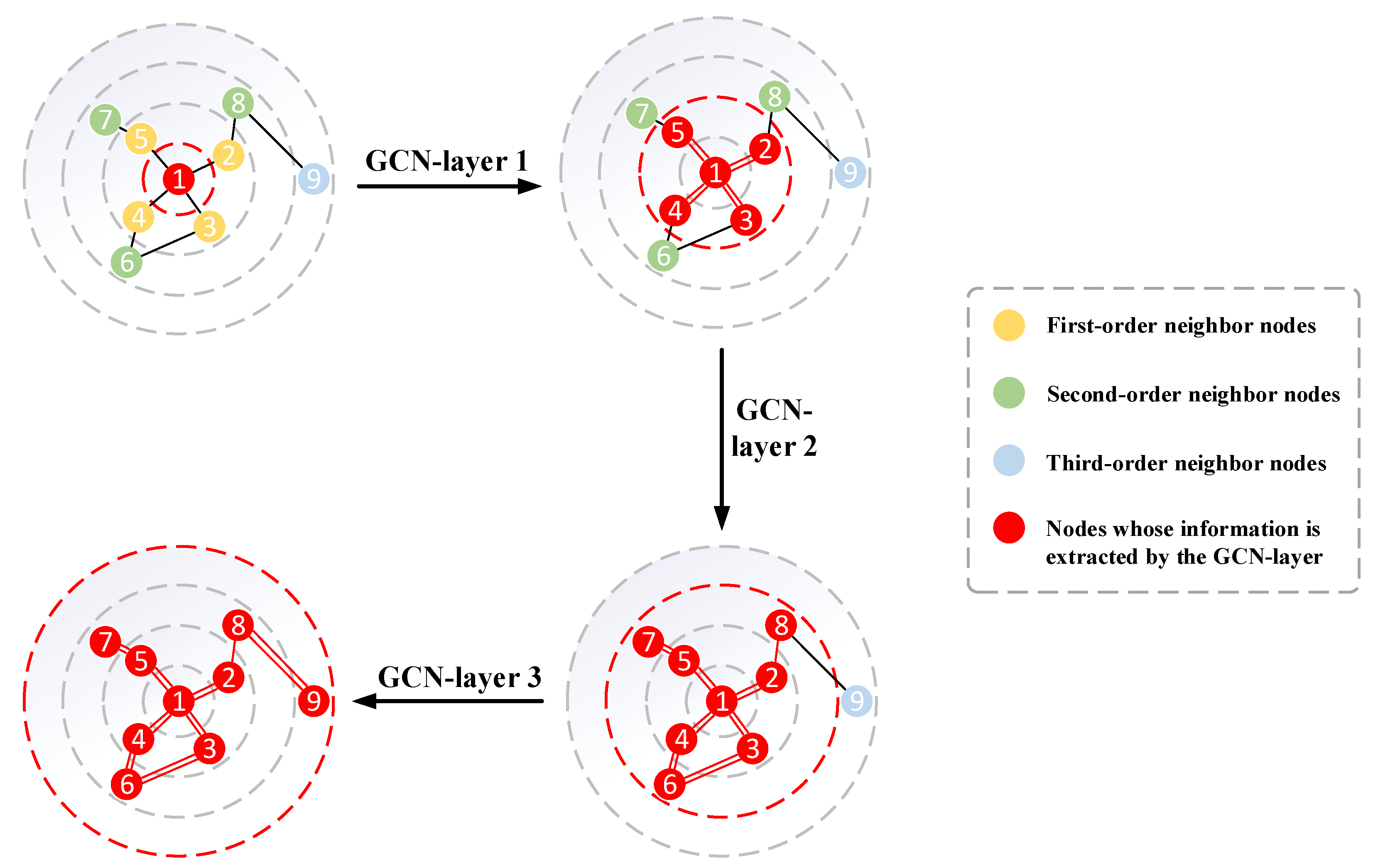
2.2.2. Mix-Jump Propagation Layer

GCN can merge a node’s information with its neighbors’ information. For each node, in order to extract its multi-order neighbors’ information, it is necessary to stack multi-layer graph convolutional layers. However, as the number of graph convolution layers increases, the node hiding state gradually converges to a single point, which means that some information of the nodes’ original state will be lost [29]. Therefore, this paper proposes the mix-jump propagation layer to cope with information flow between graph nodes, which retains a part of the nodes’ original state during the propagation, so that the nodes’ state can maintain the locality and globality after propagation. The composition relationship between the graph convolution module and the mix-jump propagation layer is shown in Figure 2.

The proposed mix-jump layer consists of two parts: information propagation and information filtering. As shown in Figure 3, it first propagates information horizontally and then filters information vertically. The information propagation part is defined as follows:

$$H^{(l+1)}=\alpha H_{in}+(1-\alpha )({\tilde{D}}^{-\frac{1}{2}}\tilde{A}{\tilde{D}}^{-\frac{1}{2}}{H}^{(l)})$$

(3)

where α is the ratio of keeping the nodes’ original state, $H_{in}$ is the hidden states output by the preceding layer, $H^{(0)}=H_{in}$. Typically, not all neighborhood information is valuable; the information filtering part is used to filter out the unimportant information generated at each jump. The information filtering part is defined as follows:

$$H_{out}={\displaystyle \sum _{l=0}^L{H}^{(l)}{W}^{(l)}}$$

(4)

where L is the depth of propagation, $H_{out}$ represents the output of this layer.

2.3. Graph Construction Module

Existing GCN methods depend on manually predefined graphical structures to achieve time series prediction. However, in most cases, there is no explicit graphical structure for the multivariate time series, and the spatial dependence between multivariate time series must be discovered from the data rather than provided as basic facts. Even if the graphical structure is available, the manually predefined graphical structure may not be optimal and should be updated during training [30]. To address this problem, based on the findings of the literature [31], graphs can be trained from the backpropagation of the loss function using gradient descent, and this paper proposes a graph construction module. This module can model multivariate time series data, treat the variables in the multivariate time series as nodes in the graph, describe the relationships between the nodes using a graph adjacency matrix, and learn and update the internal graph structure simultaneously during the training process. The basic steps of the graph construction model are as follows:

First, start with node embedding, i.e., the nodes are mapped to a low-dimensional feature space and represented as a matrix, which can be expressed as:

$$G_1=\tanh (\beta U_1{\theta }_1)$$

(5)

$$G_2=\tanh (\beta U_2{\theta }_2)$$

(6)

where U₁, U₂ represent node embedding random initialization, which will be learned during training; ${\theta }_1,{\theta }_2$ are model parameters; tanh is hyperbolic tangent function; β is the saturation rate of the activation function.

Second, it generates graph adjacency matrix using the following equation:

$$A=\mathrm{ReLu}(\tanh (\beta (G_1{G}_2^T-G_2{G}_1^T)))$$

(7)

where ReLu is a rectified linear unit that regularizes the adjacency matrix.

Finally, for each node, choose the k nodes with the strongest spatial association with it as connected nodes, and set the non-connected node weights to zero while preserving the connected node weights. For i = 1, 2, …, n, compute the A as:

$$key=nontopk(A[i,:])$$

(8)

$$A[i,key]=0$$

(9)

where n is the number of nodes in the graph, and nontopk(∙) gets the index of non-top k maximum value of a vector.

2.4. Temporal Convolution Module

The temporal dependence is another vital problem in electricity price forecasting. Recurrent neural networks (RNN) are models dedicated to sequence data; however, the architecture of RNN determines that it is prone to gradient explosion or gradient disappearance during training. LSTM [32] and GRU [33] are used to solve the above problems, but they have longer training time, more model parameters, and are prone to overfitting. Recently, temporal convolutional networks (TCN) [34] have been shown to perform significantly better than generic recurrent architectures, such as LSTM and GRU, in processing sequence data, and they exhibit longer memory than recurrent architectures with the same capacity. TCN captures the time dependence of sequence data through a one-dimension convolutional filter. In order to capture associations between temporal models with different lengths and process long time series, this paper proposes two dilated splicing layers making up a temporal convolution module. There is a tangential hyperbolic activation function behind one layer and a sigmoid activation function behind the other, both of which act as gates to control the amount of information that can be passed to the next module. The composition relationship between the dilated splicing layer and temporal convolution module is shown in Figure 4.

2.4.1. Splicing Architecture

Choosing the right convolutional kernel size is a critical step in building a convolutional network: not too small to capture long-term temporal models fully or too large to represent short-term temporal models delicately. Therefore, the convolution in this paper is performed by applying the splicing architecture method, i.e., connecting the outputs of convolution filters with different kernel sizes. Time models typically have several common cycles, such as 7, 12, and 24. Therefore, splicing architecture in improved TCN consists of four convolution kernels of sizes 1 × 2, 1 × 3, 1 × 6, and 1 × 7. These filter combinations can capture the common cycles described above. For example, the combination of filters 1 × 7 and 1 × 6 can capture cycle 12.

2.4.2. Dilated Convolution

The receptive field of the convolutional network is linearly related to the network depth and the kernel size. In order to deal with long-term sequences, it is often necessary to use deeper networks or larger filters, which will increase the complexity of the model. This paper adopts dilated convolution to reduce complication.

Dilated convolution is a convolution that skips input values of a certain step size in order to obtain a larger receptive field. [35]. It is equivalent to convolution with a larger filter that is obtained by dilating the original filter with zeros, but is significantly more efficient. Figure 5 shows dilated convolution with dilation factors 1, 2, 4, and 8. Note that dilated convolution with a dilation factor of 1 is equivalent to the standard convolution. With only a few layers of dilated convolution, the network can have a large receptive field while maintaining its computational efficiency.

2.4.3. Dilated Splicing Layer

Formally, the structure of modified TCN that incorporates splicing and dilated convolution is shown in Figure 6. For a 1D sequence input $x\in R^T$ and filters containing $f_{1\times 2}\in R^2$, $f_{1\times 3}\in R^3$, $f_{1\times 6}\in R^6$, and $f_{1\times 7}\in R^7$, the modified TCN is expressed as follows:

$$x=splice(x♦f_{1\times 2},x♦f_{1\times 3},x♦f_{1\times 6},x♦f_{1\times 7})$$

(10)

taking the output length of the largest filter as the standard, the outputs of the four filters are truncated to the same length and connected across the channel dimension, the dilated convolution operation $x♦f_{1\times k}$ on element t is defined as:

$$x♦f_{1\times k}(t)={\displaystyle \sum _{i=0}^{k-1}{f}_{1\times k}(i)x(t-d\times i)}$$

(11)

where k is the filter size, d is the dilation factor.

2.5. Residual Connections

Residual connections have been repeatedly shown to be important in maintaining the stability and improving the accuracy of TCN [36]. Formally, the residual block is defined as:

$$y=Activation(x+F(x))$$

(12)

where x and y are the input and output of the residual block, F is a series of transformations. This ensures that layers are not learning the entire transformation, but rather, changes in the identity mapping.

2.6. Model

As displayed in Figure 7, the proposed T-GCN model consists of a graph construction module, graph convolution modules, and temporal convolution modules. First, to discover latent spatial dependencies between price areas, the graph construction module computes the graph adjacency matrix by loss function and gradient descent, and then feeds it into all the graph convolution modules. Then, graph convolution modules and temporal convolution modules are interleaved to capture the spatio-temporal correlation between multivariate time series data. Figure 7 illustrates the collaboration between graph convolution modules and temporal convolution modules. To improve the stability and accuracy of the model, the residual modules are used to connect the output of temporal convolution modules and the input of the output module. Finally, the output module converts the hidden states into the required output dimension.

We observe that multi-step forecasting generates much higher losses than one-step forecasting. Therefore, in order to improve the prediction accuracy, this paper uses a training algorithm for multi-step prediction task. Based on the idea of “from easy to difficult”, the algorithm starts from solving the simplest one-step prediction task, and the number of prediction steps gradually increases with the increase of iteration times until the model can complete the more difficult multi-step prediction. The details are shown in Algorithm 1.

Algorithm 1 The training algorithm of T-GCN.

1: Input: The initialized T-GCN model f with Ω, batch size b, step size s, learning rate ζ, the price dataset O

2: set iter = 1, h = 1

3: repeat

4:           extract a batch (x ∈ Rb×T×n×D, y ∈ Rb×T’×n) from O.

5:           if iter% s = 0 and h < = T’ then

6:                     h = h + 1

7:           end if

8:           compute ŷ = f (x[:, :, :, :]; Ω)

9:           compute L = loss (ŷ [:, : h, :], y[:, : h, :])

10:         compute the stochastic gradient of Ω according to L.

11:         update model parameters Ω according to their gradients and the learning rate ζ.

12:         iter = iter + 1

13: until convergence

3. Experiments

3.1. Data Collection

This paper uses 15 regional electricity price series from the Nordic electricity market for the empirical study. The Nordic electricity market is a regional electricity market that includes several countries, such as Denmark, Sweden, and Norway. Due to geographical and demographic factors, there is a mismatch between power resources and load in the Nordic region, with cheap hydropower concentrated in northern Norway, and expensive thermal power concentrated in Denmark and Finland. In addition, the northern part of the Nordic region is sparsely populated, and the load is low, whereas the load is mainly concentrated in the densely populated and industrialized southern region. At the same time, due to climatic factors, the generation capacity of hydropower also varies seasonally, so that during the high wet season, hydropower concentrated in the northern part of Norway is delivered to the southern part, whereas during the dry season, thermal power from Denmark is delivered to the northern part. The above factors objectively contribute to the formation of the Nordic regional market, which is divided into 15 price areas, corresponding to the distribution of price areas as shown in Figure 8, with significantly different electricity price series in different price areas. Therefore, the case used in this paper can effectively reflect the validity of the proposed model.

The electricity price in the Nordic electricity market has 24 observations per day, i.e., the time interval between observations is one hour. In this paper, electricity price data for 15 price areas from 1 June 2018 to 31 August 2018, with a total of 2208 observations, are selected to demonstrate the usability of the proposed model. In addition, the first 80% of the data is defined as the training set, and the last 20% as the training set.

For market players in the electricity market, multi-step-ahead forecasting is more valuable than single-step-ahead forecasting. However, the accuracy of multi-step-ahead prediction is usually inferior to that of single-step-ahead prediction due to the accumulation of errors and the increase of uncertainty factors. [37]. This study is devoted to building a new spatio-temporal forecasting model to achieve higher accuracy multi-step-ahead electricity price forecasting.

To reduce the training time, we normalize the input data to the interval [0, 1].

3.2. Evaluation Metrics

This paper uses three common evaluation metrics to evaluate the effectiveness of the proposed model, namely, mean absolute error (MAE), root mean square error (RMSE), and mean absolute percentage error (MAPE). The computational formulas of these three evaluation metrics are provided as follows:

$$\mathrm{MAE}=\frac{1}{MN}{\displaystyle \sum _{j=1}^M{\displaystyle \sum _{i=1}^N\left|y_i^j-{\widehat{y}}_i^j\right|}}$$

(13)

$$\mathrm{RMSE}=\sqrt{\frac{1}{MN}{\displaystyle \sum _{j=1}^M{\displaystyle \sum _{i=1}^N{(y_i^j-{\widehat{y}}_i^j)}^2}}}$$

(14)

$$\mathrm{MAPE}=\frac{1}{MN}{\displaystyle \sum _{j=1}^M{\displaystyle \sum _{i=1}^N\left|\frac{y_i^j-{\widehat{y}}_i^j}{y_i^j}\right|}}$$

(15)

where $y_i^j$ and ${\widehat{y}}_i^j$ represent the real electricity price value and predicted value of the jth observation point in the ith price area, respectively. M is the number of observations in the time series; N is the number of price areas.

Specifically, smaller values of MAE, RMSE, and MAPE represent better predictions.

3.3. Experimental Results

We compare the performance of the T-GCN model with the following methods:

• Autoregressive integrated moving average model (ARIMA) [38].
• Support vector regression model (SVR) [39].
• Graph convolutional network model (GCN), see Section 2.2 for details.
• Temporal convolutional network model (TCN), see Section 2.4 for details.

The performance of the T-GCN model and other methods in the multi-step-ahead electricity price forecasting task is shown in

Table 1. Comparison of prediction performances of different models.

T	Index	ARIMA	SVR	GCN	TCN	T-GCN
1-h	MAE	5.1537	3.3396	2.2115	2.0220	1.5979
	RMSE	8.1943	5.3433	3.4941	3.1745	2.4799
	MAPE(%)	9.33	6.04	3.82	3.63	2.82
2-h	MAE	6.2299	5.1288	3.2331	2.5614	2.2652
	RMSE	9.6862	8.2573	5.0759	4.0162	3.4912
	MAPE(%)	11.15	9.23	5.68	4.51	3.98
3-h	MAE	6.2376	5.9534	3.8765	2.9550	2.6800
	RMSE	9.7306	9.4063	6.0473	4.6157	4.1127
	MAPE(%)	11.17	10.71	7.01	5.38	4.71
4-h	MAE	6.2539	6.2182	4.0456	3.3649	2.9038
	RMSE	9.6935	9.9491	6.2707	5.2156	4.4272
	MAPE(%)	11.19	11.31	7.20	6.07	5.12

. It is not difficult to see that compared with other methods, the T-GCN model has achieved the best evaluation index in all forecasting tasks, which proves its effectiveness in multi-regional electricity price forecasting tasks. Figure 9 provides three histograms of MAE, RMSE, and MAPE values based on different models, which present more intuitively the performance differences between the different methods.

3.4. Discussion

(1)

Higher prediction accuracy. It was found that neural network-based approaches that include temporal feature modeling, such as T-GCN models and TCN models, typically have better prediction accuracy than other methods, such as ARIMA models and SVR models. For example, for a 1-h electricity price prediction task, compared with the ARIMA model, MAE errors of the T-GCN model and TCN model are reduced by 68.99% and 60.76%, respectively; RMSE errors are reduced by 69.73% and 61.25%, respectively. Compared with the SVR model, MAE errors of the T-GCN model and TCN model are reduced by 52.15% and 39.45%, and RMSE errors are reduced by 53.59% and 40.59%. This is mainly due to the difficulty of methods such as ARIMA and SVR to handle complex non-stationary time series data.

(2)

Spatio-temporal prediction capability. We compared the T-GCN model with the GCN model and TCN model to verify the ability of the T-GCN model to capture its temporal and spatial characteristics from electricity price data of multiple price areas. As shown in Figure 9, the T-GCN model based on spatio-temporal features has higher prediction accuracy than the GCN and TCN models based on a single feature, indicating that the T-GCN model can capture spatio-temporal features from the electricity price data. For example, the MAE error of the T-GCN model is reduced by about 27.74% and 29.94% for the 1-h and 2-h prediction tasks, respectively, compared with the GCN model that considered only spatial features, indicating that the T-GCN model can capture spatial dependence. Compared with the TCN model, which only considers temporal characteristics, the MAE error of the T-GCN model is reduced by about 20.97% and 11.56% for 1-h and 2-h electricity price forecasts, respectively, indicating that the T-GCN model is able to capture temporal correlation well.

(3)

Long-term forecasting capability. The T-GCN model can obtain the best prediction performance by training, regardless of the change of the prediction horizon, indicating that the proposed model is insensitive to the prediction horizons and has strong stability. Therefore, the T-GCN model can be used for both short-term and long-term forecasting. Figure 9 shows the comparison of RMSE of different models, with the T-GCN model achieving the best results for different prediction horizons. Figure 10 shows the changes of T-GCN’s performance at different forecasting horizons. It can be seen that the trend of increasing error is small and has some stability.

3.5. Further Illustration of the Model

To better understand the contribution of the constructed graph adjacency matrix, Figure 11 shows the geographic location of the three price areas, LV, EE, and FI, where LV is the area geographically bordering EE, and FI is the constructed maximum weighted neighbor of EE. We plot the raw price data for these three regions in Figure 12.We observe that LV is closer to EE on the map, but the price data are less correlated. In contrast, the constructed maximum weighted neighbor FI is further away from EE, but their electricity price data are strongly correlated. Based on the flow data for the period, as shown in Figure 11, FI is the area that delivers the most power to EE, 5331.3 MWh more than LV, which shows that the T-GCN model can mine the potential dependence between variables through multivariate time-series data.

4. Conclusions

In this paper, we propose an effective method to capture the intrinsic dependencies among multiple electricity price series and build a new electricity price prediction model, T-GCN, to solve the electricity price prediction problem through a graph-based deep learning approach. On the one hand, the connection structure between nodes in the graph is captured by GCN to obtain spatial dependencies; on the other hand, TCN is used to capture the dynamic changes of nodes’ own attributes to obtain temporal dependencies. Evaluated on a Nordic electricity market dataset containing 15 price areas, the T-GCN model achieves better performance in different forecasting ranges compared with the ARIMA model, SVR model, GCN model, and TCN model. In conclusion, the T-GCN model successfully captures the spatio-temporal characteristics of multiple electricity price data and realizes high-precision forecasting. From the mathematical point of view, this is because our method has strong fitting ability for multiple time series with potential dependence, and can better map the relationship between input and output. Therefore, it can be applied to other multivariable time series prediction tasks with hidden dependency, such as multi region wind power generation prediction, distributed photovoltaic output prediction, etc.

References

1. Liu, J.; Wang, J.; Cardinal, J. Evolution and reform of UK electricity market. Renew. Sustain. Energy Rev. 2022, 161, 112317. [Google Scholar] [CrossRef]
2. Shamsi, M.; Cuffe, P. A Prediction Market Trading Strategy to Hedge Financial Risks of Wind Power Producers in Electricity Markets. IEEE Trans. Power Syst. 2021, 36, 4513–4523. [Google Scholar] [CrossRef]
3. Mashlakov, A.; Kuronen, T.; Lensu, L.; Kaarna, A.; Honkapuro, S. Assessing the performance of deep learning models for multivariate probabilistic energy forecasting. Appl. Energ. 2021, 285, 116405. [Google Scholar] [CrossRef]
4. Sun, W.; Huang, C. A carbon price prediction model based on secondary decomposition algorithm and optimized back propagation neural network. J. Clean. Prod. 2020, 243, 118671. [Google Scholar] [CrossRef]
5. Fraunholz, C.; Kraft, E.; Keles, D.; Fichtner, W. Advanced price forecasting in agent-based electricity market simulation. Appl. Energ. 2021, 290, 116688. [Google Scholar] [CrossRef]
6. Lu, H.; Ma, X.; Ma, M.; Zhu, S. Energy price prediction using data-driven models: A decade review. Comput. Sci. Rev. 2021, 39, 100356. [Google Scholar] [CrossRef]
7. Rabiya, K.; Nadeem, J. A survey on hyperparameters optimization algorithms of forecasting models in smart grid. Sustain. Cities Soc. 2020, 61, 102275. [Google Scholar]
8. Lago, J.; Marcjasz, G.; De Schutter, B.; Weron, R. Forecasting day-ahead electricity prices: A review of state-of-the-art algorithms, best practices and an open-access benchmark. Appl. Energ. 2021, 293, 116983. [Google Scholar] [CrossRef]
9. Sujit, K.D.; Pradipta, K.D. Short-term mixed electricity demand and price forecasting using adaptive autoregressive moving average and functional link neural network. J. Mod. Power Syst. Clean 2019, 7, 1241–1255. [Google Scholar]
10. Radhakrishnan, A.C.; Anupam, M.; Mitch, C.; Hossein, S.; Timothy, M.H.; Jeremy, L.; Prakash, R. A Multi-Stage Price Forecasting Model for Day-Ahead Electricity Markets. Forecasting 2018, 1, 26–46. [Google Scholar]
11. Shibalal, M. Estimating and forecasting residential electricity demand in Odisha. J. Public Aff. 2020, 20, e2065. [Google Scholar]
12. Zheng, L.; Yushan, W.; Jiayu, W.; Lin, Z.; Jian, S.; Xu, W. Short-term electricity price forecasting G-LSTM model and economic dispatch for distribution system. IOP Conf. Ser. Earth Environ. Sci. 2020, 467, 012186. [Google Scholar]
13. Wendong, Y.; Jianzhou, W.; Rui, W. Research and Application of a Novel Hybrid Model Based on Data Selection and Artificial Intelligence Algorithm for Short Term Load Forecasting. Entropy 2017, 19, 52. [Google Scholar]
14. Lehna, M.; Scheller, F.; Herwartz, H. Forecasting day-ahead electricity prices: A comparison of time series and neural network models taking external regressors into account. Energ Econ. 2022, 106, 105742. [Google Scholar] [CrossRef]
15. Li, W.; Becker, D.M. Day-ahead electricity price prediction applying hybrid models of LSTM-based deep learning methods and feature selection algorithms under consideration of market coupling. Energy 2021, 237, 121543. [Google Scholar] [CrossRef]
16. Aslam, S.; Ayub, N.; Farooq, U.; Alvi, M.J.; Albogamy, F.R.; Rukh, G.; Haider, S.I.; Azar, A.T.; Bukhsh, R. Towards Electric Price and Load Forecasting Using CNN-Based Ensembler in Smart Grid. Sustainability 2021, 13, 12653. [Google Scholar] [CrossRef]
17. Yang, H.; Schell, K.R. Real-time electricity price forecasting of wind farms with deep neural network transfer learning and hybrid datasets. Appl. Energ. 2021, 299, 117242. [Google Scholar] [CrossRef]
18. Yiyuan, C.; Yufeng, W.; Jianhua, M.; Qun, J. BRIM: An Accurate Electricity Spot Price Prediction Scheme-Based Bidirectional Recurrent Neural Network and Integrated Market. Energies 2019, 12, 2241. [Google Scholar]
19. Xiao, C.; Sutanto, D.; Muttaqi, K.M.; Zhang, M.; Meng, K.; Dong, Z.Y. Online Sequential Extreme Learning Machine Algorithm for Better Predispatch Electricity Price Forecasting Grids. IEEE Trans. Ind. Appl. 2021, 57, 1860–1871. [Google Scholar] [CrossRef]
20. Yi-Kuang, C.; Hardi, K.; Philipp, A.G.; Jon, G.K.; Klaus, S.; Hans, R.; Torjus, F.B. The role of cross-border power transmission in a renewable-rich power system—A model analysis for Northwestern Europe. J. Environ. Manag. 2020, 261, 110194. [Google Scholar]
21. Jorge, M.U.; Stephanía, M.; Montserrat, G. Characterizing electricity market integration in Nord Pool. Energy 2020, 208, 118368. [Google Scholar]
22. Egerer, J.; Grimm, V.; Kleinert, T.; Schmidt, M.; Zöttl, G. The impact of neighboring markets on renewable locations, transmission expansion, and generation investment. Eur. J. Oper Res. 2020, 292, 696–713. [Google Scholar] [CrossRef]
23. Tessoni, V.; Amoretti, M. Advanced statistical and machine learning methods for multi-step multivariate time series forecasting in predictive maintenance. Procedia Comput. Sci. 2022, 200, 748–757. [Google Scholar] [CrossRef]
24. Guokun, L.; Wei-Cheng, C.; Yiming, Y.; Hanxiao, L. Modeling Long- and Short-Term Temporal Patterns with Deep Neural Networks. In Proceedings of the 41st International ACM SIGIR Conference on Research & Development in Information Retrieval, Ann Arbor, MI, USA, 8–12 July 2018; pp. 95–104. [Google Scholar] [CrossRef] [Green Version]
25. Shih, S.Y.; Sun, F.K.; Lee, H.Y. Temporal pattern attention for multivariate time series forecasting. Mach. Learn. 2019, 108, 1421–1441. [Google Scholar] [CrossRef] [Green Version]
26. Zhang, Z.; Cui, P.; Zhu, W. Deep Learning on Graphs: A Survey. IEEE Trans. Knowl. Data Eng. 2020, 34, 249–270. [Google Scholar] [CrossRef] [Green Version]
27. Asif, N.A.; Sarker, Y.; Chakrabortty, R.K.; Ryan, M.J.; Ahamed, M.H.; Saha, D.K.; Badal, F.R.; Das, S.K.; Ali, M.F.; Moyeen, S.I.; et al. Graph Neural Network: A Comprehensive Review on Non-Euclidean Space. IEEE Access 2021, 9, 60588–60606. [Google Scholar] [CrossRef]
28. Cui, Z.; Henrickson, K.; Ke, R.; Wang, Y. Traffic Graph Convolutional Recurrent Neural Network: A Deep Learning Framework for Network-Scale Traffic Learning and Forecasting. IEEE Trans. Intell. Transp. Syst. 2019, 21, 4883–4894. [Google Scholar] [CrossRef] [Green Version]
29. Zhou, X.; Wang, H. The Generalization Error of Graph Convolutional Networks May Enlarge with More Layers. Neurocomputing 2020, 424, 97–106. [Google Scholar] [CrossRef]
30. Wu, Z.; Pan, S.; Chen, F.; Long, G.; Zhang, C.; Yu, P.S. A Comprehensive Survey on Graph Neural Networks. IEEE Trans. Neural Netw. Learn. Syst. 2020, 32, 4–24. [Google Scholar] [CrossRef] [Green Version]
31. Lin, G.; Kang, X.; Liao, K.; Zhao, F.; Chen, Y. Deep graph learning for semi-supervised classification. Pattern Recogn. 2021, 118, 108039. [Google Scholar] [CrossRef]
32. Hochreiter, S.; Schmidhuber, J. Long short-term memory. Neural Comput. 1997, 9, 1735–1780. [Google Scholar] [CrossRef]
33. KyungHyun, C.; Bart, V.M.; Dzmitry, B.; Yoshua, B. On the Properties of Neural Machine Translation: Encoder-Decoder Approaches. arXiv 2014, arXiv:1409.1259. [Google Scholar]
34. Bai, S.; Kolter, J.Z.; Koltun, V. An Empirical Evaluation of Generic Convolutional and Recurrent Networks for Sequence Modeling. arXiv 2018, arXiv:1803.01271. [Google Scholar]
35. Oord, A.V.D.; Dieleman, S.; Zen, H.; Simonyan, K.; Vinyals, O.; Graves, A.; Kalchbrenner, N.; Senior, A.; Kavukcuoglu, K. WaveNet: A Generative Model for Raw Audio. arXiv 2016, arXiv:1609.03499. [Google Scholar]
36. Kaiming, H.; Xiangyu, Z.; Shaoqing, R.; Jian, S. Deep Residual Learning for Image Recognition. arXiv 2015, arXiv:1512.03385. [Google Scholar]
37. Souhaib, B.T.; Gianluca, B.; Amir, F.A.; Antti, S. A review and comparison of strategies for multi-step ahead time series forecasting based on the NN5 forecasting competition. Expert Syst. Appl. 2012, 39, 7067–7083. [Google Scholar]
38. Patrícia, R.; Nicolau, S.; Rui, R. Performance of state space and ARIMA models for consumer retail sales forecasting. Robot. Comput. Integr. Manuf. 2015, 34, 151–163. [Google Scholar]
39. Alex, J.S.; Bernhard, S.L. A tutorial on support vector regression. Stat. Comput. 2004, 14, 199–222. [Google Scholar]
Figure 1. Schematic diagram of GCN extracting spatial features.
Mathematics 10 02366 g001
Figure 2. Graph convolution module structure.
Mathematics 10 02366 g002
Figure 3. Mix-jump propagation layer.
Mathematics 10 02366 g003
Figure 4. Temporal convolution module structure.
Mathematics 10 02366 g004
Figure 5. Visualization of a stack of dilated convolutional layers.
Mathematics 10 02366 g005
Figure 6. Dilated splicing layer.
Mathematics 10 02366 g006
Figure 7. The framework of T-GCN.
Mathematics 10 02366 g007
Figure 8. Price area distribution of Nordic electricity market.
Mathematics 10 02366 g008
Figure 9. Performance comparison of different models in terms of MAE, RMSE, MAPE.
Mathematics 10 02366 g009
Figure 10. The visualization results for different prediction horizons.
Mathematics 10 02366 g010
Figure 11. Geographical location of the three price areas, FI, EE, and LV.
Mathematics 10 02366 g011
Figure 12. Electricity price data for the three areas, EE, LV, and FI.
Mathematics 10 02366 g012