Modelling Bimodal Data Using a Multivariate Triangular-Linked Distribution

Abstract

Bimodal distributions have rarely been studied although they appear frequently in datasets. We develop a novel bimodal distribution based on the triangular distribution and then expand it to the multivariate case using a Gaussian copula. To determine the goodness of fit of the univariate model, we use the Kolmogorov–Smirnov (KS) and Cramér–von Mises (CVM) tests. The contributions of this work are that a simplistic yet robust distribution was developed to deal with bimodality in data, a multivariate distribution was developed as a generalisation of this univariate distribution using a Gaussian copula, a comparison between parametric and semi-parametric approaches to modelling bimodality is given, and an R package called btld is developed from the workings of this paper.

1. Introduction

Bimodality in data can be described as the presence of two distinct modes and many examples of bimodal data can be found in nature. Bimodality can occur in a variety of circumstances. Firstly, it can occur when there are two or more latent attributes of the data which might result in bimodality. For instance, if we consider the frequency of cars crossing a bridge in a 24 h period, two modes manifest because two peak traffic hours are latently reflected [1]. Moreover, as determined by [2], if we review the spread of tree cover in a desert, specific attributes about the geography in the area latently influence the spread of the trees. In both cases, the bimodality in the data is generated from a single population with multiple latent attributes.

Secondly, bimodality could occur if there are attributes of sub-populations present in the data. An example of this can be the spread of height amongst college students. If we ignore gender and just record the height of students, we can expect bimodality to reflect in histograms of the data.

A common approach to handle bimodality is to use mixture distributions, which are semi-parametric models that yield density estimations as well as clustering solutions [3]. This approach requires the estimation of five parameters: the means and standard deviations of the two normal distribution, and the mixing parameter. Alternatively, one could fit a bimodal parametric distribution to the data.

Both of these approaches pose benefits and challenges to the modeller. Bimodal parametric models result in a mathematical formulation for the cumulative distribution function (CDF) which is convenient for hypothesis testing and calculation of confidence intervals. The challenge is to find the exact estimates of the parameters. Mixture models come with relaxed parametric assumptions, but the choice of number of components is not always intuitive and the computational complexity increases as the number of components increases [4].

In this paper, we propose a mathematically concise and simplistic approach to modelling bimodal data. We use the well-known triangular distribution as the initial point of reference and then extend it to what we call the bimodal triangular-linked distribution (BTLD). This newly formulated distribution accommodates bimodality without considering mixture models.

We generalise this distribution to a multivariate context using a Gaussian copula. Copulas join or “couple” univariate distribution functions, say $F\left(x\right)$ and $G\left(y\right)$, to form a multivariate distribution function $H(x,y)=C\left(F\right(x),G(x\left)\right)$. Modelling the joint distribution is done by mixing the marginal distributions using a bivariate function (known as a copula) $C:(u,v)\to C(u,v)$ which captures and reflects the dependence pattern of X and Y [5].

To determine the goodness of fit of the univariate model, we use the Kolmogorov–Smirnov (KS) and Cramér–von Mises (CVM) tests. The KS test is a nonparametric test that uses the maximum absolute distances between the empirical distribution and the proposed null distribution to test if the proposed null distribution truly fits the data in the test [3,6]. The CVM test is an alternative to the KS test and has been suggested to use the data more effectively [7,8]. The null hypothesis is the same for both tests and the discrepancy in the tests lies in the way that the test statistics, d for the KS and ${\omega }^2$ for the CVM, are calculated [8]. We use both tests to ensure the consistency of our testing framework. The contributions of this paper are as follows:

1.

A simplistic yet robust distribution geared to handle bimodality in its parameters is developed from a fusion of uniform and triangular distributions which we called the bimodal triangular-linked (BTL) distribution,

2.

A multivariate extension is developed using a copula to model the dependance structures of multiple variables. A simulation is shown as well as comparison to a multivariate Gaussian mixture model (GMM),

3.

A comparison between parametric and semi-parametric approaches to dealing with bimodality in data is illustrated in the form of an application to gene expression data,

4.

An R package is constructed from the workings of this paper called btld. An explanation of the functionality of this package is included in Appendix B. All generations and computations regarding the BTL are done using this package.

The rest of the paper is structured as follows: In Section 2, we review related work in the fields of bimodal distributions and mixture model. Section 3 covers important background theory on the triangular model. This section also motivates the use of Kolmogorov–Smirnov and Cramér–von Mises test as goodness of fit tests. The bimodal triangular-linked model with its statistical properties is introduced in Section 4. The generalisation to the multivariate context is enabled through copulas which are introduced in Section 3.3. The multivariate generalisation, the Multivariate triangular-linked distribution is introduced in Section 5 after which its application is illustrated in Section 6. Section 7 concludes with a discussion of results and future work.

2. Related Work

Bimodal data are very relevant as it occurs often in practice. The two main approaches used to to model such data are the use of mixture models or special parametric distributions which inherently capture bimodality. Mixture models are semi-parametric models that yield density estimations [3]. Although not strictly bimodal, mixture models may yield bimodality in the densities if the data provide for it. Mixture models are constructed by taking a weighted sum of two or more distributions. There is a vast number of distributions to choose from, thus when it comes to creating a mixture model, there are virtually endless possibilities and the final decision will typically depend on the data and the needs of the practitioner. Sheng et al. [9] demonstrated that mixture models can be used in pharmacodynamic studies in which bimodal count data arise. They found that the two generalized Poisson mixture model was the best fit for their bimodal dataset consisting of the number of times that a rodent licked an oral medication in a palatability study. Bimodal distributions have also been used in cancer studies. Irace and Batatia [10] demonstrated the effectiveness of the univariate and bivariate mixtures of Poisson distributions in automatic image segmentation of 4-D bimodal PET-CT images used for cancer diagnoses. A mixture of bivariate negative binomial-normal distributions has also been considered for the same purpose [11]. In genetics, Gaussian mixture models have been used to identify genes with bimodal expression patterns in tumors [12]. Other applications where mixture models have been used for bimodal data include modelling ratings from Tripadvisor.com [13],

Over the last two decades, many researchers have proposed new distributions for bimodal data based on the skew normal distribution [14]. The skew normal distribution is an extension of the normal distribution which includes an additional parameter to induce asymmetry. Based on this idea of modifying a normal distribution, Elal-Olivero [15] developed a new skewed distribution called the alpha-skewed-normal (ASN) distribution by introducing a parameter which allows for the added flexibility of modelling both unimodal and bimodal data. A further extension to the ASN that allowed at most four modes, called the alpha-beta skewed normal (ABSN) distribution, was later proposed by Shafiei et al. [16]. This ABSN was used to model the bimodal acidity indices of lakes in Northeastern United States [16]. More recently, using a methodology advocated by Balakrishnan [17], the Balakrishnan-alpha-skewed-normal (BASN₂) distribution was proposed [18] as well as its extension, the Balakrishnan alpha-beta skewed normal (BABSN₂) [19] which is able to model up to four modes. A BASN₂ distribution was fit to a bimodal dataset consisting of 69 samples of N latitude degrees from world lakes and was found to outperform several other skewed distributions, including the ASN and ABSN, based on AIC and BIC [19]. This approach of using skewed distributions to model bimodal data is very common. Other examples of such distributions include the alpha-skew Laplace distribution [20], the alpha-skew-logistic distribution [21,22], bimodal skew-elliptical distributions [23], flexible generalized skew normal and t distributions [24], as well as some multivariate skewed distributions presented in [25,26,27]. See also [28,29,30,31,32,33,34,35,36,37] for other related work. Skewed distributions have also been used in the construction of mixture models. For instance, the skew normal mixture model (SNMIX) was shown to produce batter AIC and BIC scores than traditional normal mixture models on two real-world datasets [38]. To address the SNMIX’s possible lack of robustness in the presence of outliers, Lin et al. [39] proposed the skew t mixture (STMIX).

3. Background Theory

We first provide background theory on the triangular distribution, goodness-of-fit tests, and copulas which are main points of reference for the rest of the paper.

3.1. Triangular Distribution

The Triangular distribution on the $(0,1)$ space has one parameter $\theta$ also lying in $(0,1)$. Taken from Kotz and van Dorp [40], the probability density function (PDF) for the triangular distribution is defined as

$$f\left(x\right)=\left\{\begin{array}{cc}\frac{2x}{\theta }\hfill & 0\le x\le \theta \hfill \\ \frac{2(1-x)}{1-\theta }\hfill & \theta \le x\le 1\hfill \\ 0\hfill & \mathrm{otherwise}.\hfill \end{array}\right.$$

(1)

The cumulative distribution function (CDF) is obtained by integrating Equation (1),

$$F\left(x\right)=\left\{\begin{array}{cc}0\hfill & x<0\hfill \\ \frac{x^2}{\theta }\hfill & 0\le x<\theta \hfill \\ 1-\frac{{(1-x)}^2}{1-\theta }\hfill & \theta \le x<1\hfill \\ 1\hfill & x\ge 1.\hfill \end{array}\right.$$

(2)

The inverse CDF (ICDF) is,

$$F^{-1}\left(u\right)=\left\{\begin{array}{cc}\sqrt{\theta u}\hfill & 0\le u<\theta \hfill \\ 1-\sqrt{(1-\theta )(1-u)}\hfill & \theta \le u<1\hfill \\ 0\hfill & \mathrm{Otherwise}.\hfill \end{array}\right.$$

(3)

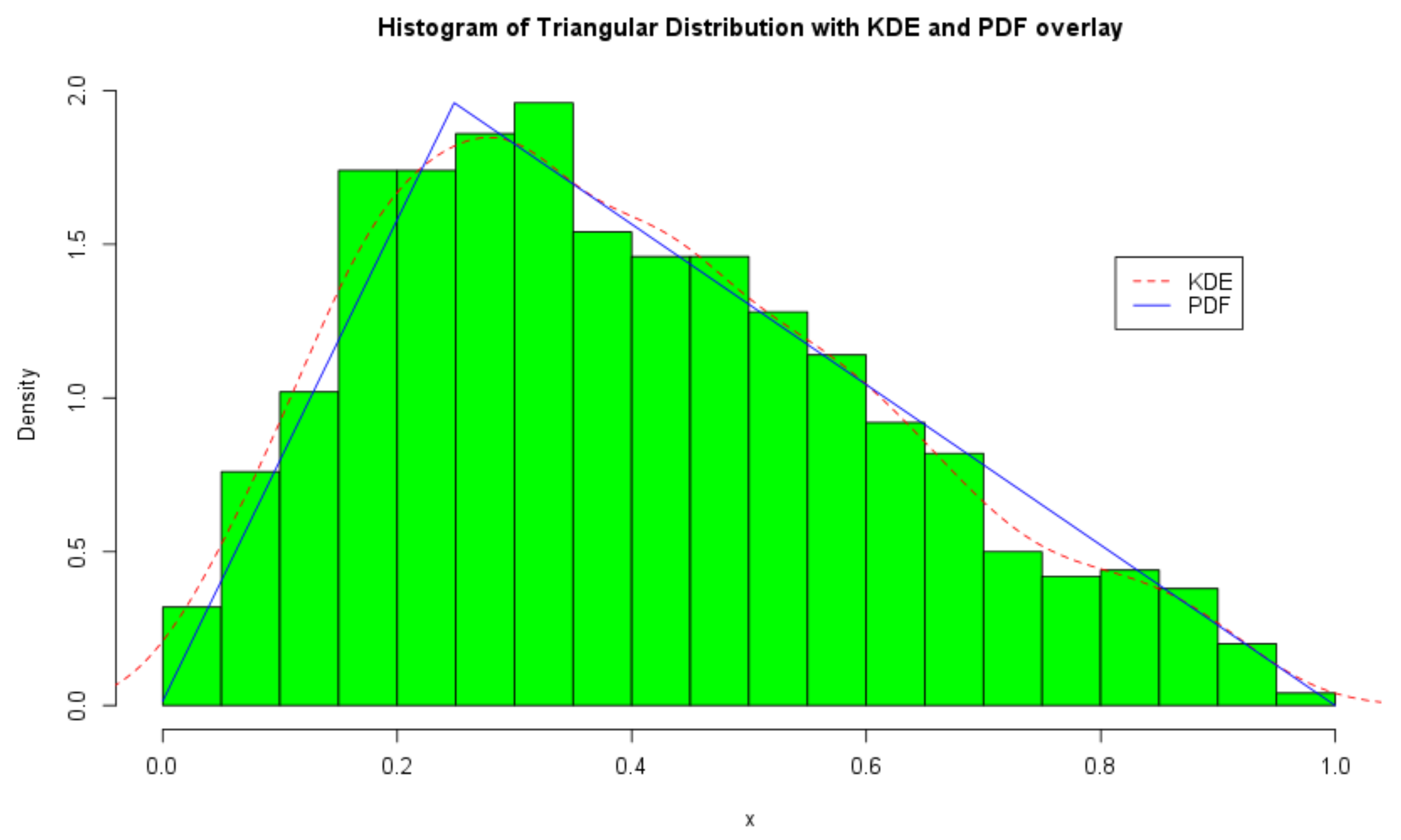
The ICDF transform method [41] is used to simulate random variables from the triangular distribution as illustrated in Figure 1. For clarity, we overlay a kernel density estimate and the PDF of the triangular distribution on the histogram of the random variables.

Figure 1. Histogram and density plots of the triangular distribution with $\theta =0.25$.

3.2. Kolmogorov–Smirnov Goodness-of-Fit

In many cases it is not possible to make assumptions about the underlying distribution of a given dataset and one needs to consider non-parametric or semi-parametric methods. A non-parametric model postulates that observations come from some distribution function F not constrained by any parameters. However, the interpretability of these models are not so clear and semi-parametric models might be considered as a compromise [3]. First, consider the estimate of a distribution function, i.e., the empirical cumulative distribution function, $F_n^{*}\left(x\right)$. It is formally calculated, at some point x, by taking the proportion of sample observations less than or equal to that point,

$$F_n^{*}\left(x\right)\frac{1}{n}\sum _{i=1}^{n}I(X_i\le x)$$

(4)

where $I\left(·\right)$ is the indicator function. The indicator function is defined as

$$I(X_i\le x)=\left\{\begin{array}{cc}0\hfill & \mathrm{if}{X}_i\le x\hfill \\ 1\hfill & \mathrm{if}{X}_i>x\hfill \end{array}\right.$$

(5)

It has been proven that the empirical CDF is an unbiased and consistent estimator of the true CDF. That is to say the following properties can be drawn about the estimator,

• $\left(F_n^{*}\left(x\right)\right)=F\left(x\right)$
• $\left(F_n^{*}\left(x\right)\right)=\frac{F\left(x\right)(1-F(x\left)\right)}{n}\therefore$ as $n⟶\infty \Rightarrow \left(F_n^{*}\left(x\right)\right)⟶0$ such that $F_n^{*}\left(x\right)$ is an unbiased and consistent estimator for $F\left(x\right)$

The Kolmogorov–Smirnov (KS) test of goodness of fit is a non-parametric test that uses a proposed distribution function $F_0\left(x\right)$ versus the observed cumulative function $S_n\left(x\right)$, alternatively known as the empirical CDF (ECDF). Our null hypothesis is that the sample can be modelled using $F_0\left(x\right)$. The crux of this test is that we expect the observed CDF and the proposed CDF to be very close to each other for all N observations. If the distributions are too distinct from each other then we can conclude that the proposed distribution is not appropriate for modelling the sample. That is, we reject our null hypothesis [6]. Our hypotheses are generally constructed as follows,

$$\begin{array}{ccc}\hfill H_0:F\left(x\right)& =& F_0\left(x\right),\hfill \\ \hfill H_a:F\left(x\right)& \ne & F_0\left(x\right).\hfill \end{array}$$

Formally, if $F_0\left(x\right)$ is the population cumulative distribution function, and $S_N\left(X\right)=k/N$ where k is the cumulative index of x, then let Kolmogorov’s D be defined as follows,

$$D=\underset{x\in (-\infty ,\infty )}{sup}|F_0\left(x\right)-S_N\left(x\right)|.$$

(6)

Large values of this statistic suggest with a high level of probability that we will reject the null hypothesis and the converse applies for small values [3]. Furthermore, note that Equation (6) is independent of $F_0\left(x\right)$ if $F_0$ is continuous. To make conclusions about D we use tables that yield critical points of the distribution of D for differing sample sizes. We reject the null hypothesis if $D>d_{\alpha }\left(N\right)$ where $\alpha$ is the level of significance for our test.

3.3. Copulas

Most standard probability distributions are generalised to the multivariate context such as the multivariate Gaussian distribution. The multivariate generalisation is important in order to model dependencies between variables. We run into the problem that multivariate generalisations do not exist for all distributions and furthermore, one might want to model the dependency between two different distributions for which the mathematical formulation does not exist either.

Copulas are mathematical functions that describe the dependency structure between a finite set of univariate marginal distributions [42]. The main idea is that marginal properties can be separated from correlation properties. Under the hood, copulas are multivariate distributions with uniform marginals. Using the inverse probability transform [41,42] any distribution can be generated from the uniform distribution.

The basis of taking a set of correlated uniform random variates (which is the copula itself) and transforming these into a multivariate distribution with arbitrary marginals is based on Sklar’s theorem which proofs that we can extract the correlation structure from marginal distributions and used to create a set of marginals and a copula [42,43].

The dependence structure is independent of the marginals and is fully described by the copula. Furthermore, transformations that preserve the ranks will preserve the copula, since the copulas are linked to the ranks of random variables. The main purpose of a copula is to describe the dependence between the marginal distributions. Furthermore, the copula can be used to calculate conditional probabilities and predictions. At first sight, this might not seem to make a huge difference, but the effect is typically amplified in the tails of the dependency structure.

The most common copula is the Gaussian copula which forms part of the collection of copulas known as elliptical copulas from the shape the copula structure makes.Another elliptical copula is the Student’s t copula [44]. Popular copulas in the Archimedian family of copulas include the Gumbel, Frank copula, the Cook-Johnson copula and the Clayton copula.

Alternative approaches to measuring the dependence structures of copulas may be taken instead of the widely known Pearson’s linear correlation coefficient because the structure of the marginals can change the linear correlation coefficient, but not so for non-parametric dependence measures such as Kendall’s tau and Spearman’s rho. These measures capture the dependency inherent in the copula structure, not that just presented by the marginals. One may opt to use the Clayton copula if one is interested in having a high lower tail dependence structure. This is useful for modelling unlikely events, i.e., ones that tend to occur in the lower tail. Conversely, for a Gaussian copula, the dependence breaks down in the tails [45].

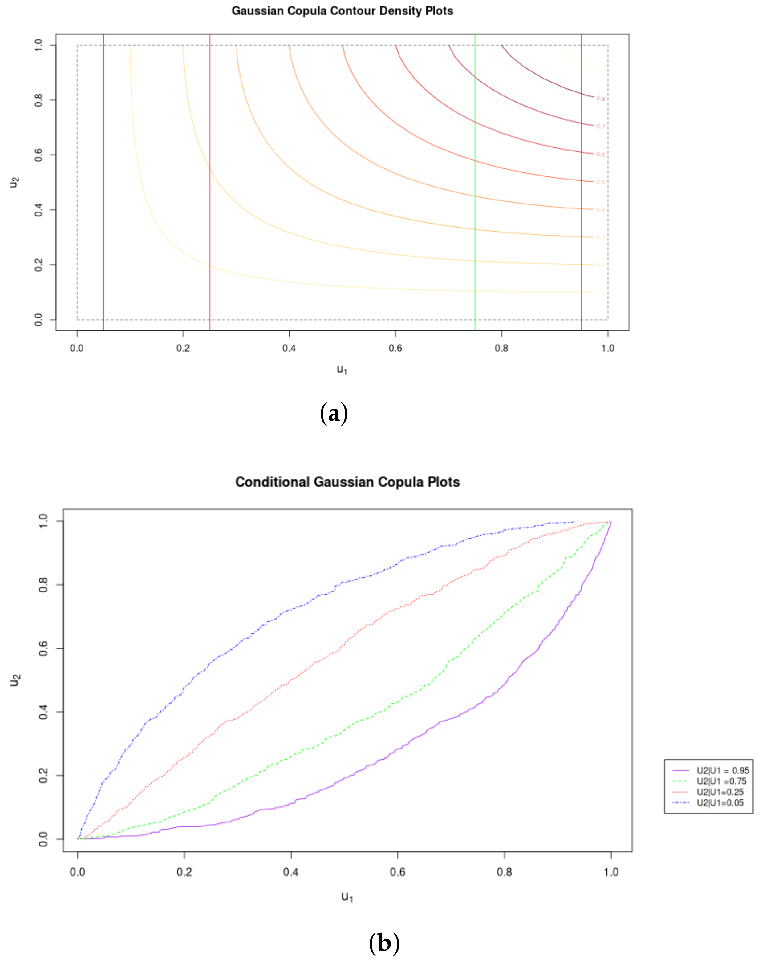
Figure 2 illustrates the conditional distributions that can be generated from copulas: Given a particular observation in one of the marginals, we can determine the probability and cumulative distributions for the other.

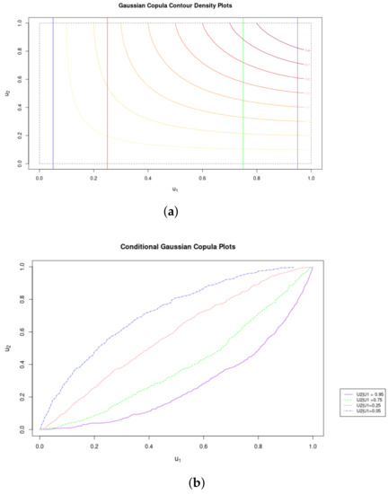
Figure 2. Conditonal Copula CDFs. (a) Contours of Gaussian Coupla with Marginal Distributions (See legend in (b). (b) Marginal Conditional Distributions of the Gaussian Copula.

4. Bimodal Triangular-Linked Distribution

We derive the Bimodal triangular-linked ($\mathcal{BTL}$) distribution as an extension of the triangular PDF defined in Equation (1). The mode of the triangular distribution is $\theta$. Pulling the two triangle legs apart—left and right of the mode—results in a distribution with two modes, say ${\theta }_1$ and ${\theta }_2$. The introduction of the two parameters ${\alpha }_1$ and ${\alpha }_2$ has the implication that the density is zero between the two modes ${\theta }_1$ and ${\theta }_2$. If we allow the density between the modes, denoted as $f\left(x\right)={\alpha }_0$, to follow a uniform distribution as part of the probability density over this area such that ${\int }_0^{1}f\left(x\right)dx=1$, it implies that ${\alpha }_0=(1-\frac{1}{2}{\theta }_1{\alpha }_1-\frac{1}{2}{(1-{\theta }_2)}^2{\alpha }_2)/{\theta }_2-{\theta }_1$. That is, the uniform density ${\alpha }_0$ can be rewritten in terms of parameters of the distribution. Note that $\mathbf{\theta }$ = $[{\theta }_1,{\theta }_2$] is defined such that it satisfies the following,

$$0<{\theta }_1\le {\theta }_2<1.$$

Therefore, if we substitute these values of $\mathbf{\theta }$ and introduce multiplicative scaling factors ${\alpha }_1$ and ${\alpha }_2$ into Equation (1), we find that the BTL distribution takes on form,

$$f\left(x\right)=\left\{\begin{array}{cc}\frac{{\alpha }_{1}x}{{\theta }_1}\hfill & 0\le x\le {\theta }_1\hfill \\ {\alpha }_0\hfill & {\theta }_1\le x\le {\theta }_2\hfill \\ \frac{{\alpha }_2(1-x)}{1-{\theta }_2}\hfill & {\theta }_2\le x\le 1\hfill \\ 0\hfill & \mathrm{otherwise}.\hfill \end{array}\right.$$

(7)

4.1. Triangular-Linked Statistics

Some statistics of the TL distribution—apart from being bimodal with modes ${\theta }_1$ and ${\theta }_2$ are the first and second moments. The mean is:

$$E\left(X\right)=\frac{1}{4}{\alpha }_1{\theta }_1^4+\frac{1}{3}{\alpha }_2({\theta }_2-{\theta }_1)+\frac{1}{2}{\alpha }_2({\theta }_2^2-1)-\frac{1}{3}{\alpha }_0({\theta }_2^3-1)$$

(8)

and

$${\left\{E\left(X\right)\right\}}^2=\frac{1}{3}{\alpha }_1{\theta }_1^2+\frac{1}{3}{\alpha }_2({\theta }_2^3-{\theta }_1^3)-\frac{1}{3}{\alpha }_2{(1-{\theta }_2)}^3-\frac{1}{2}{\alpha }_0{(1-{\theta }_2)}^4.$$

(9)

Also useful to note is that if ${\theta }_1=0$ and ${\theta }_2=1$, the distribution becomes a UNF $(0,1)$ with ${\alpha }_1=1,{\alpha }_2=1$.

4.2. Derivation of the CDF

Using Equation (7), we can derive the CDF for the BTL distribution.

Proof. 

For $x<0:$

$$\begin{array}{ccc}\hfill F\left(x\right)& =& {\int }_{-\infty }^{x}f\left(t\right)dt\hfill \\ & =& {\int }_{-\infty }^{x}0dt\hfill \\ & =& 0\hfill \end{array}$$

(10)

For $0\le x<{\theta }_1:$

$$\begin{array}{ccc}\hfill F\left(x\right)& =& {\int }_{-\infty }^{x}f\left(t\right)dt\hfill \\ & =& {\int }_0^x\frac{{\alpha }_{1}t}{{\theta }_1}dt+F\left(0\right)\hfill \\ & =& \frac{{\alpha }_1{t}^2}{2{\theta }_1}{|}_0^x+0\hfill \\ & =& {\alpha }_1\frac{{\left(x\right)}^2-{\left(0\right)}^2}{2{\theta }_1}\hfill \\ & =& \frac{{\alpha }_1{x}^2}{2{\theta }_1}\hfill \end{array}$$

(11)

For ${\theta }_1\le x<{\theta }_2:$

$$\begin{array}{ccc}\hfill F\left(x\right)& =& {\int }_{-\infty }^{x}f\left(t\right)dt\hfill \\ & =& {\int }_{{\theta }_1}^x{\alpha }_{0}dt+F\left({\theta }_1\right)\hfill \\ & =& {\alpha }_{0}t{|}_{{\theta }_1}^x+\frac{{\alpha }_1{\theta }_1^2}{2{\theta }_1}\hfill \\ & =& {\alpha }_0(x-{\theta }_1)+\frac{{\alpha }_1{\theta }_1}{2}\hfill \end{array}$$

(12)

For ${\theta }_2\le x<1:$

$$\begin{array}{ccc}\hfill F\left(x\right)& =& {\int }_{-\infty }^{x}f\left(t\right)dt\hfill \\ & =& {\int }_{{\theta }_2}^{x}f\left(t\right)+F\left({\theta }_2\right)\hfill \\ & =& {\int }_{{\theta }_2}^x\frac{{\alpha }_2(1-t)}{1-{\theta }_2}+{\alpha }_0({\theta }_2-{\theta }_1)+\frac{{\alpha }_1{\theta }_1}{2}\hfill \\ & =& \frac{-{\alpha }_2{(1-t)}^2}{2(1-{\theta }_2)}{|}_{{\theta }_2}^x+{\alpha }_0({\theta }_2-{\theta }_1)+\frac{{\alpha }_1{\theta }_1}{2}\hfill \\ & =& \frac{-{\alpha }_2{(1-x)}^2}{2(1-{\theta }_2)}+\frac{{\alpha }_2{(1-{\theta }_2)}^2}{2(1-{\theta }_2)}+{\alpha }_0({\theta }_2-{\theta }_1)+\frac{{\alpha }_1{\theta }_1}{2}\hfill \\ & =& \frac{-{\alpha }_2{(1-x)}^2}{2(1-{\theta }_2)}+\underset{=1}{\underbrace{\frac{{\alpha }_2(1-{\theta }_2)}{2}+{\alpha }_0({\theta }_2-{\theta }_1)+\frac{{\alpha }_1{\theta }_1}{2}}}\hfill \\ & =& 1-\frac{{\alpha }_2{(1-x)}^2}{2(1-{\theta }_2)}\hfill \end{array}$$

(13)

Note that the expression that gets reduced to 1 in the second last line of the above derivation is proven in Appendix A. For $x\ge 1:$

$$\begin{array}{ccc}\hfill F\left(x\right)& =& {\int }_{-\infty }^{x}f\left(t\right)dt\hfill \\ & =& {\int }_1^{x}0dt+F\left(1\right)\hfill \\ & =& 1-\frac{{\alpha }_2{(1-1)}^2}{2(1-{\theta }_2)}\hfill \\ & =& 1\hfill \end{array}$$

(14)

Therefore the CDF of the $\mathcal{BTL}$ is,

$$F\left(x\right)=\left\{\begin{array}{cc}0\hfill & x\le 0\hfill \\ \frac{{\alpha }_1{x}^2}{2{\theta }_1}\hfill & 0<x\le {\theta }_1\hfill \\ {\alpha }_0(x-{\theta }_1)+\frac{{\alpha }_1{\theta }_1}{2}\hfill & {\theta }_1<x\le {\theta }_2\hfill \\ 1-\frac{{\alpha }_2{(1-x)}^2}{2(1-{\theta }_2)}\hfill & {\theta }_2<x\le 1\hfill \\ 1\hfill & x>1\hfill \end{array}\right.$$

(15)

□

4.2.1. Sample Estimates of Parameters

The CDF values of ${\theta }_1$ and ${\theta }_2$ can be determined using Equation (2). Thus,

$$\begin{array}{ccc}\hfill F\left({\theta }_1\right)={\alpha }_1\frac{{\theta }_1^2}{2{\theta }_1}={\alpha }_1\frac{{\theta }_1}{2}& \Rightarrow & {\alpha }_1=\frac{2F\left({\theta }_1\right)}{{\theta }_1}\hfill \\ \hfill F\left({\theta }_2\right)={\alpha }_0({\theta }_2-{\theta }_1)+\frac{{\alpha }_1{\theta }_1}{2}& \Rightarrow & F\left({\theta }_2\right)=1-\frac{{\alpha }_2(1-{\theta }_2)}{2}\hfill \end{array}$$

(16)

$$\begin{array}{ccc}& \Rightarrow & {\alpha }_2=\frac{2(1-F\left({\theta }_2\right))}{1-{\theta }_2}\hfill \end{array}$$

(17)

Note that the expression for $F\left({\theta }_2\right)$ is derived from Equation (A2) in Appendix A. These values are pivotal in determining sample estimates of ${\mathbf{\alpha }}_i$ and ${\mathbf{\theta }}_i$. If the empirical CDF of the function is known, the breakpoints on the plot will be indicative of the modal parameters ${\mathbf{\theta }}_i$. Once the breakpoint values ${\widehat{\theta }}_1$ and ${\widehat{\theta }}_2$, and their corresponding function values $F\left({\widehat{\theta }}_1\right)$ and $F\left({\widehat{\theta }}_2\right)$ are determined, it is trivial to determine the scaling parameters ${\mathbf{\alpha }}_i$ using the formulae derived above.

4.2.2. Derivation of the ICDF, $F^{-1}\left(u\right)$

Proof. 

Let $U\sim \mathcal{U}(0,1)$. Then

$$\begin{array}{ccc}\hfill \mathrm{For}0\le u\le F\left({\theta }_1\right):u& =& F\left(F^{-1}\left(u\right)\right)\hfill \\ \hfill u& =& \frac{{\alpha }_1{F}^{-1}{\left(u\right)}^2}{2{\theta }_1}\hfill \\ \hfill 2{\theta }_{1}u& =& {\alpha }_1{F}^{-1}{\left(u\right)}^2\hfill \\ \hfill \sqrt{\frac{2{\theta }_{1}u}{{\alpha }_1}}& =& F^{-1}\left(u\right)\hfill \end{array}$$

(18)

$$\begin{array}{ccc}\hfill \mathrm{For}F\left({\theta }_1\right)\le u\le F\left({\theta }_2\right):u& =& F\left(F^{-1}\left(u\right)\right)\hfill \\ \hfill u& =& \begin{array}{c}\hfill {\alpha }_0(F^{-1}\left(u\right)-{\theta }_1)\\ \hfill +\frac{{\alpha }_1{\theta }_1}{2}\end{array}\hfill \\ \hfill \frac{u-\frac{{\alpha }_1{\theta }_1}{2}}{{\alpha }_0}& =& (F^{-1}\left(u\right)-{\theta }_1)\hfill \\ \hfill {\theta }_1+\frac{u-\frac{{\alpha }_1{\theta }_1}{2}}{{\alpha }_0}& =& F^{-1}\left(u\right)\hfill \end{array}$$

(19)

$$\begin{array}{ccc}\hfill \mathrm{For}F\left({\theta }_2\right)\le u\le 1:u& =& F\left(F^{-1}\left(u\right)\right)\hfill \\ \hfill u& =& 1-\frac{{\alpha }_2{(1-F^{-1}\left(u\right))}^2}{2(1-{\theta }_2)}\hfill \\ \hfill 2(1-{\theta }_2)(1-u)& =& {\alpha }_2{(1-F^{-1}\left(u\right))}^2\hfill \\ \hfill 1-\sqrt{\frac{2(1-{\theta }_2)(1-u)}{{\alpha }_2}}& =& F^{-1}\left(u\right)\hfill \end{array}$$

(20)

Therefore the ICDF of the BTL distribution is,

$$F^{-1}\left(u\right)=\left\{\begin{array}{cc}\sqrt{\frac{2{\theta }_{1}u}{{\alpha }_1}}\hfill & 0\le u\le F\left({\theta }_1\right)\hfill \\ {\theta }_1+\frac{u-\frac{{\alpha }_1{\theta }_1}{2}}{{\alpha }_0}\hfill & F\left({\theta }_1\right)\le u\le F\left({\theta }_2\right)\hfill \\ 1-\sqrt{\frac{2(1-{\theta }_2)(1-u)}{{\alpha }_2}}\hfill & F\left({\theta }_2\right)\le u\le 1\hfill \\ 0\hfill & \mathrm{Otherwise}.\hfill \end{array}\right.$$

(21)

□

Using the ICDF, we can generate the random variates from the $\mathcal{BTL}$ distribution which is illustrated in Figure 3. To showcase the exact shape of the BTL, we overlay the PDF of the generated variates as well as a KDE estimate. This is done to illustrate the exact bimodal distribution as well as the approximate bimodal distribution.

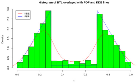
Figure 3. Histogram and Density plots of $\mathcal{BTL}$ Distribution with ${\theta }_1=0.3,{\theta }_2=0.8,{\alpha }_1={\alpha }_2=3$.

4.2.3. Goodness of Fit Test

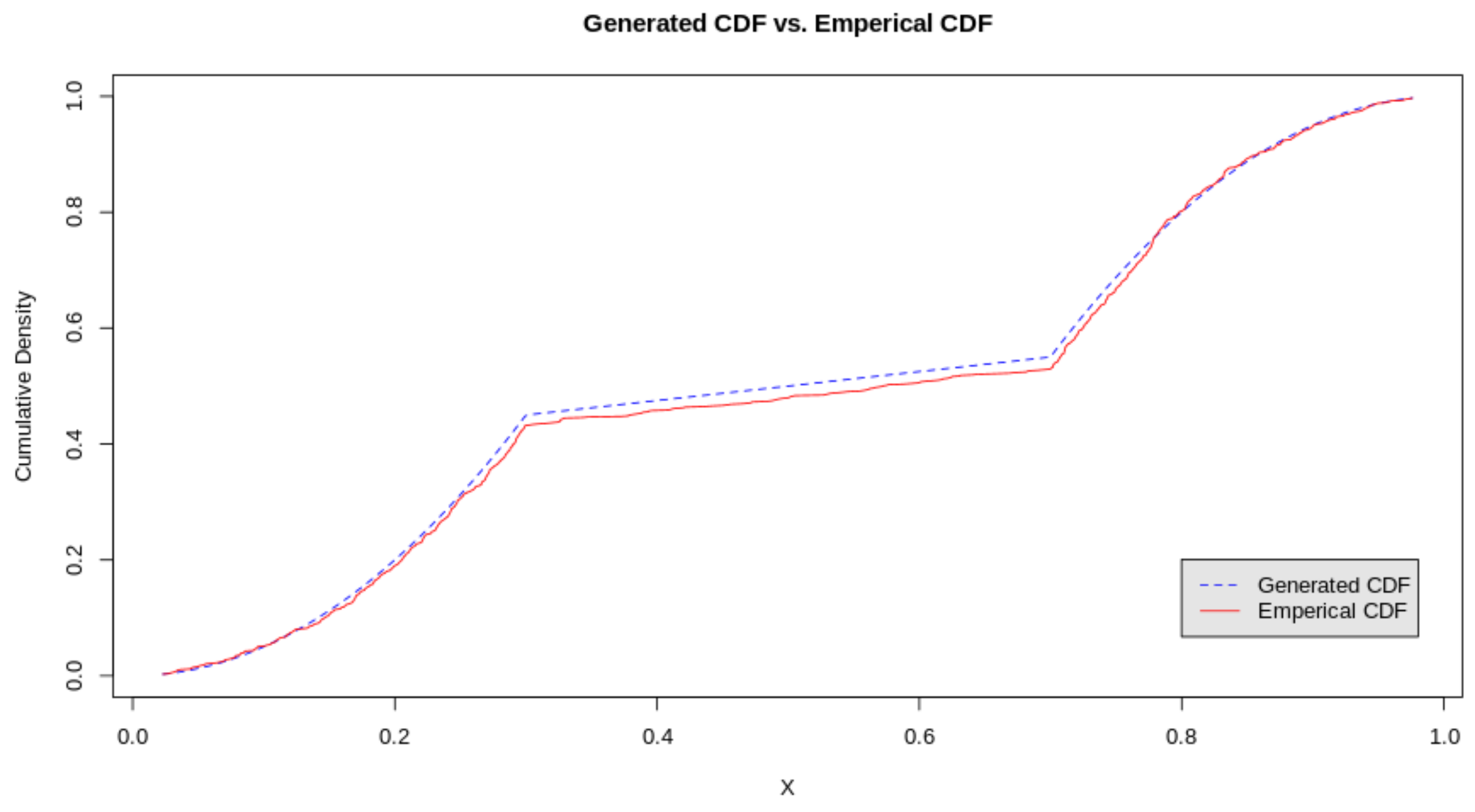
We continue with the simulated example to illustrate the goodness of fit tests for the BTL distribution. Given a simulated sample $x_1,\dots ,x_n$ of size n from the TL $(\theta ,\alpha )$ distribution, the estimation of the parameters is fairly easy using the empirical estimate of $F\left(x\right)$ which is shown in Figure 4. It is almost identical to the true df. Testing the fit of the model was conducted in R for simulated data from the bimodal triangular-linked distribution. The null hypothesis and alternative hypotheses for both cases are presented as follows:

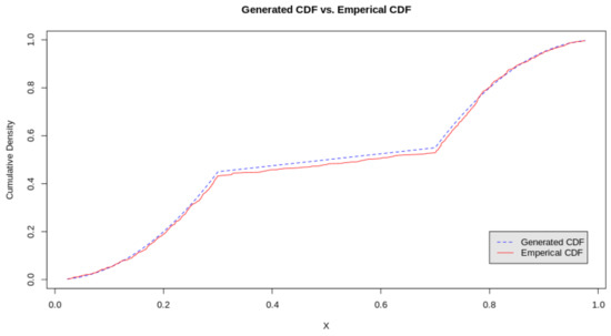
Figure 4. Graphical illustration of the KS Test for bimodal univariate case.

• $H_0^{Case1}$: the distribution, $F_0\left(x\right)$, follows a BTL distribution with parameters ${\theta }_1,{\theta }_2,{\alpha }_1,{\alpha }_2$
• $H_a^{Case1}$: the distribution does not follow a BTL distribution

The test can be conducted using p-values as well where a specified level of significance is used. The null hypothesis is rejected if $p<\alpha$. Illustrated in Figure 3, the KS-test statistic is observed to be $D=0.02$ which is quite small. Using goftest, we calculate the p-value = $P(D\ge q)$ = 0.6264 which is larger than even a lenient significance level of $\alpha =0.1$. Therefore, we do not reject the null.

5. Multivariate Triangular-Linked Distribution

Copulas equip us with the mathematics to generalise the Bimodal triangular-linked distribution to the multivariate case and we use the theory above to derive the multivariate triangular-linked (MVTL), $\mathcal{MVTL}$, distribution. Let $\mathbf{U}$ be a random Gaussian copula, $C_P^{Gauss}\left(\mathbf{u}\right)$, with $u_i={\varphi }_i\left(X_i\right)$, by the probability integral transform, [46] being the marginals where $\mathbf{X}\sim {\mathcal{MVN}}_d({\mathbf{0}}_{d\times 1},{\mathbf{P}}_{d\times d})$[42], N is the sample size we are considering and d represents the dimensionality of the random variables. By the standard inverse transform [46], let $Y_i=F\left(u_i\right)$ where the marginals $Y_i\sim \mathcal{BTL}({\mathbf{\theta }}_i,{\mathbf{\alpha }}_i)$, for $i=1,\cdots ,d$. Note that ${\mathbf{\theta }}_i=[{\theta }_{1i},{\theta }_{2i}]$ and ${\mathbf{\alpha }}_i=[{\alpha }_{1i},{\alpha }_{2i}]$. Therefore, let the distribution of $\mathbf{Y}$ be defined as follows

$${\mathit{Y}}_{n\times d}\sim \mathcal{MVTL}({\Theta }_{d\times 2},{\mathit{A}}_{d\times 2},{\mathit{R}}_{d\times d})$$

(22)

where ${\Theta }_{d\times 2}$ is a d-by-2 matrix containing the modal parameters; ${\mathit{A}}_{d\times 2}$ is the d-by-2 matrix containing the scaling factors for the distribution (explained in previous sections) and; ${\mathit{R}}_{d\times d})$ is the positive definite correlation matrix, with dimensions of d-by-d, of the Gaussian copula required to generate this multivariate distribution. Fitting this distribution as a proposed model implies we must determine sample estimates. We explain how to do this below.

• ${\mathit{R}}_{d\times d}$ can be estimated by calculating the sample correlation matrix $\widehat{\mathit{R}}=\left(\mathbf{Y}\right)$. Pearson’s correlation coefficient is calculated and used as the sample estimate.
• To determine the modes, they can be read off the ECDF at the break points ${\widehat{\theta }}_{i1}$ and ${\widehat{\theta }}_{i2}$. These points correspond to estimates of the CDF, $F\left({\widehat{\theta }}_{i1}\right)$ and $F\left({\widehat{\theta }}_{i2}\right)$.
• The scale parameters estimates ${\widehat{\alpha }}_{i1}$ and ${\widehat{\alpha }}_{i2}$, can be determined using Equations (16) and (17), respectively. After some algebraic manipulation of these equations, formulae for these parameters can be determined.

Generated Example

Let the parameter and correlation matrices be defined as follows:

$$\mathit{A}=\left[\begin{array}{cc}1& 5\\ 3& 3\\ 5& 1\end{array}\right],\Theta =\left[\begin{array}{cc}0.3& 0.7\\ 0.3& 0.7\\ 0.3& 0.7\end{array}\right]\mathrm{and}\mathit{R}=\left[\begin{array}{ccc}1& 0.5& 0.5\\ 0.5& 1& 0.5\\ 0.5& 0.5& 1\end{array}\right].$$

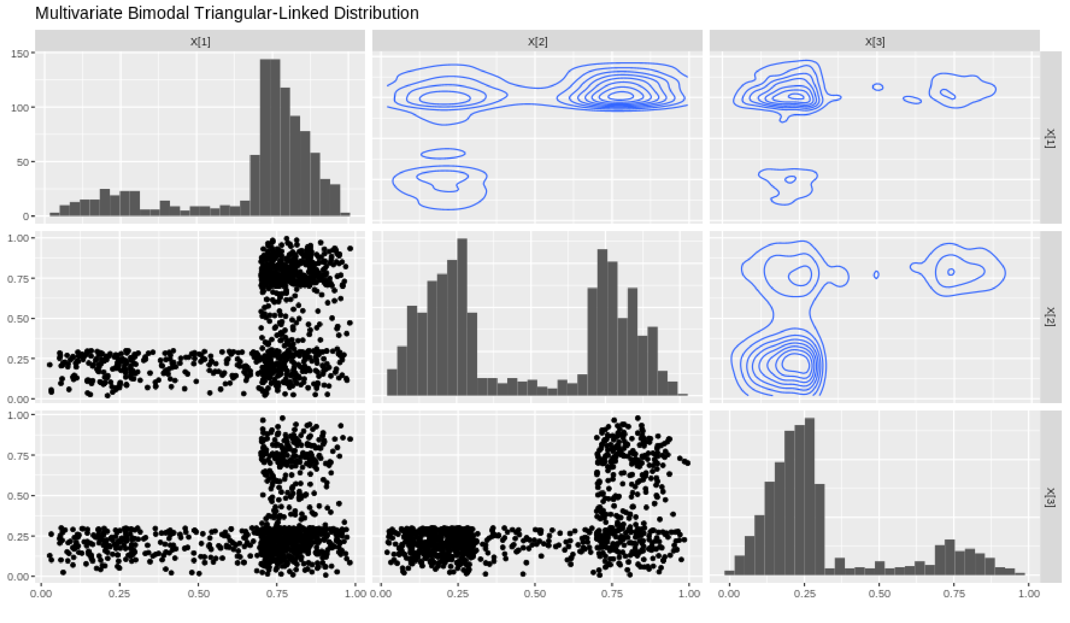
A dataset of size 1000 is simulated and a matrix plot is constructed in Figure 5 for $\mathit{X}\sim \mathcal{MVTL}(\mathit{A},\Theta ,\mathit{R})$ so as to showcase the marginal distributions of X, their shape and contours. In the lower triangular section we have scatterplots of all the marginals of $\mathbf{X}$ which we will denote as $X_1\sim \mathcal{BTL}(0.3,0.7,1,5)$ , $X_2\sim \mathcal{BTL}(0.3,0.7,3,3)$ and $X_3\sim \mathcal{BTL}(0.3,0.7,5,1).$

Figure 5. MVTL matrix plot with marginals $X_1$, $X_2$, $X_3$.

The ECDFs of the marginals are plotted in Figure 6. This plot, which we call the H-plot, is used to read off the density values associated with the mode parameters. Let $\widehat{\Theta }$ denote the observed estimate of $\Theta$. $\widehat{\Theta }$ and their associated density values, $F\left(\widehat{\Theta }\right)$, are determined from the breakpoints for each ECDF.

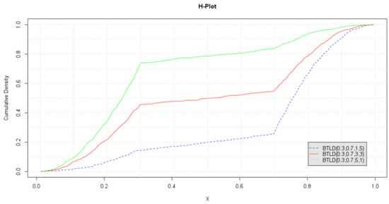
Figure 6. Empirical marginal CDFs of $\mathbf{X}$.

Therefore,

$$\widehat{\Theta }=\left[\begin{array}{cc}0.27& 0.7\\ 0.3& 0.7\\ 0.3& 0.7\end{array}\right],F\left(\widehat{\Theta }\right)=\left[\begin{array}{cc}0.17& 0.23\\ 0.43& 0.53\\ 0.73& 0.82\end{array}\right]\mathrm{and}\widehat{\mathbf{R}}=\left[\begin{array}{ccc}1& 0.5124& 0.2503\\ 0.5124& 1& 0.5377\\ 0.2503& 0.5377& 1\end{array}\right].$$

where $\widehat{\mathbf{R}}$ is the Pearson correlation coefficient of the observed data. Finally, the scale parameters are determined using the expressions obtained in Equations (16) and (). Therefore, the estimate of A, i.e., $\widehat{\mathbf{A}}$, is as follows,

$$\widehat{\mathbf{A}}=\left[\begin{array}{cc}1.2593& 5.1333\\ 2.8667& 3.1333\\ 4.8667& 1.2\end{array}\right]$$

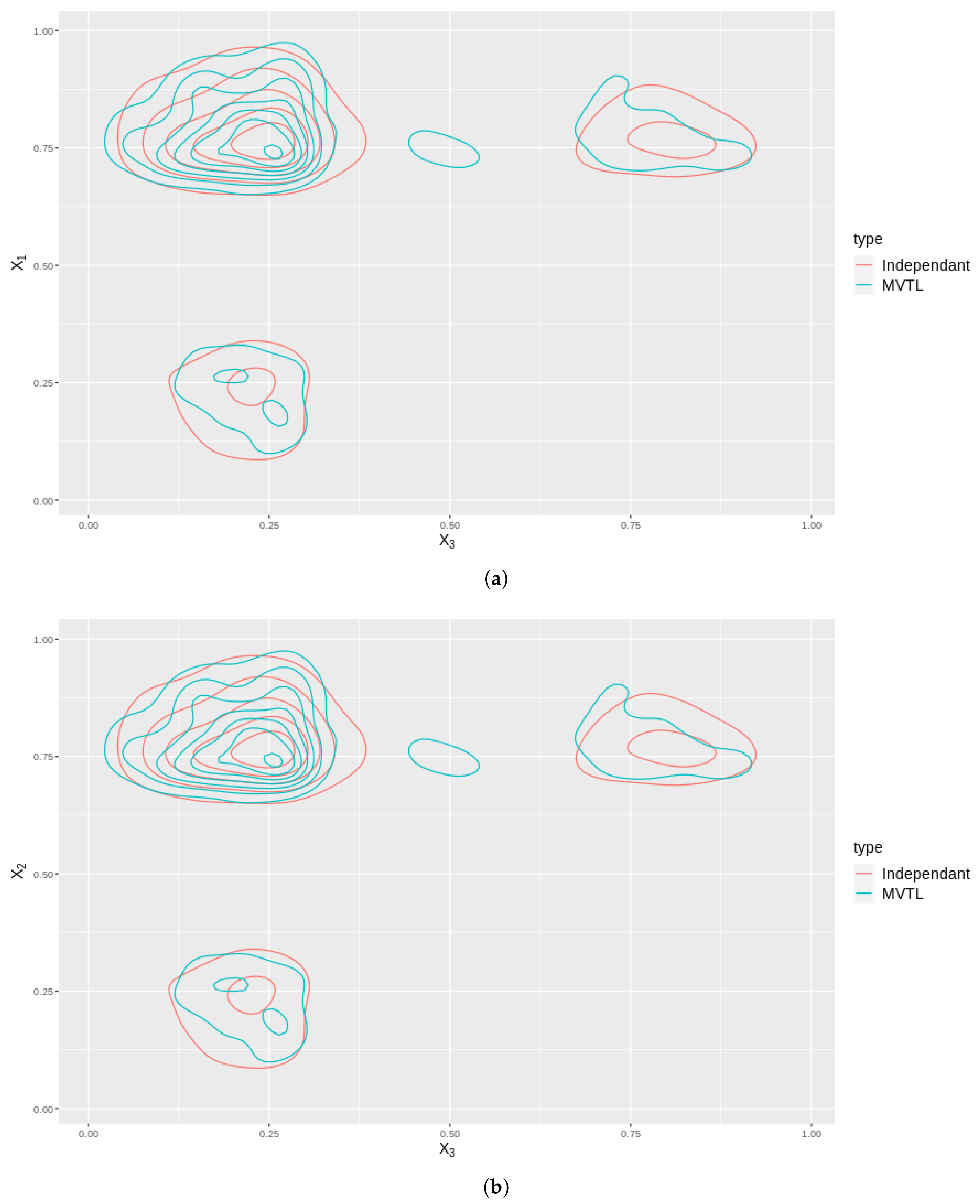
As an illustration, we plot the contours in 2D for two cases: one where we have a MVTL and the dependance structure is captured by a Gaussian copula, and; two, where the BTL marginals are independant. The distributions of these cases are plotted for all the variable $X_1$, $X_2$ and $X_3$ shown in Figure 7. Note that these contours are not the same which means that by modelling the distribution using a copula, better captures any dependance structures inherent in the data.

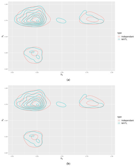
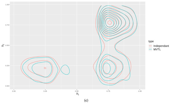
Figure 7. These subfigures are bivariate density plots for variables $X_1$, $X_2$ and $X_3$ plotted against themselves in exhaustive pairs. The plots consider the cases when they independently generated (Red contours) and the case when they are generated using a copula (Blue contours). (a) Contour plot of $X_1$ against $X_3$. (b) Contour plot of $X_2$ against $X_3$. (c) Contour plot of $X_1$ against $X_2$.

6. Application

6.1. Gene Expression Data

Gene expression data have been directed towards a better understanding of a diverse range of biological processes which can then be used to determine associations between genetic information. If bimodality in the gene expressions are identified, then this can be used to extract interesting insights into biological attributes of a particular cancer associated with the tumor. The data we will use are extracted using developed software [12], which is written in R. These data consist of expression and clinical data from 25 different tumor types which is in turn harvested from the Cancer Genome Atlas (https://portal.gdc.cancer.gov/ accessed on 5 September 2021). In total the authors of [12], get expression values measured in Fragments by Exon Kilobase per Millions of Mapped Fragments values (FPKM), for just under 25,000 genes which yields more than 10 million observations.

In the paper presented by Justino, Gaussian mixture models (GMMs) is used to model the overall density of the bimodal genes and provide a clustering solution. The GMM, as highlighted in chapter in modelling the bimodal data, is that it allows one to extract an overall density function for the bimodal data. We will consider the overall density modelled by a GMM against the overall density modelled by the BTL. Since GMMs yield clustering solutions as well as overall density functions, it could be a heavy handed approach if there is no meaningful interpretation in the clustering solution. Furthermore, one could quite easily reach an overfitted and overparameterized model by using a k-component mixture model [47].

6.2. BTL vs. GMM

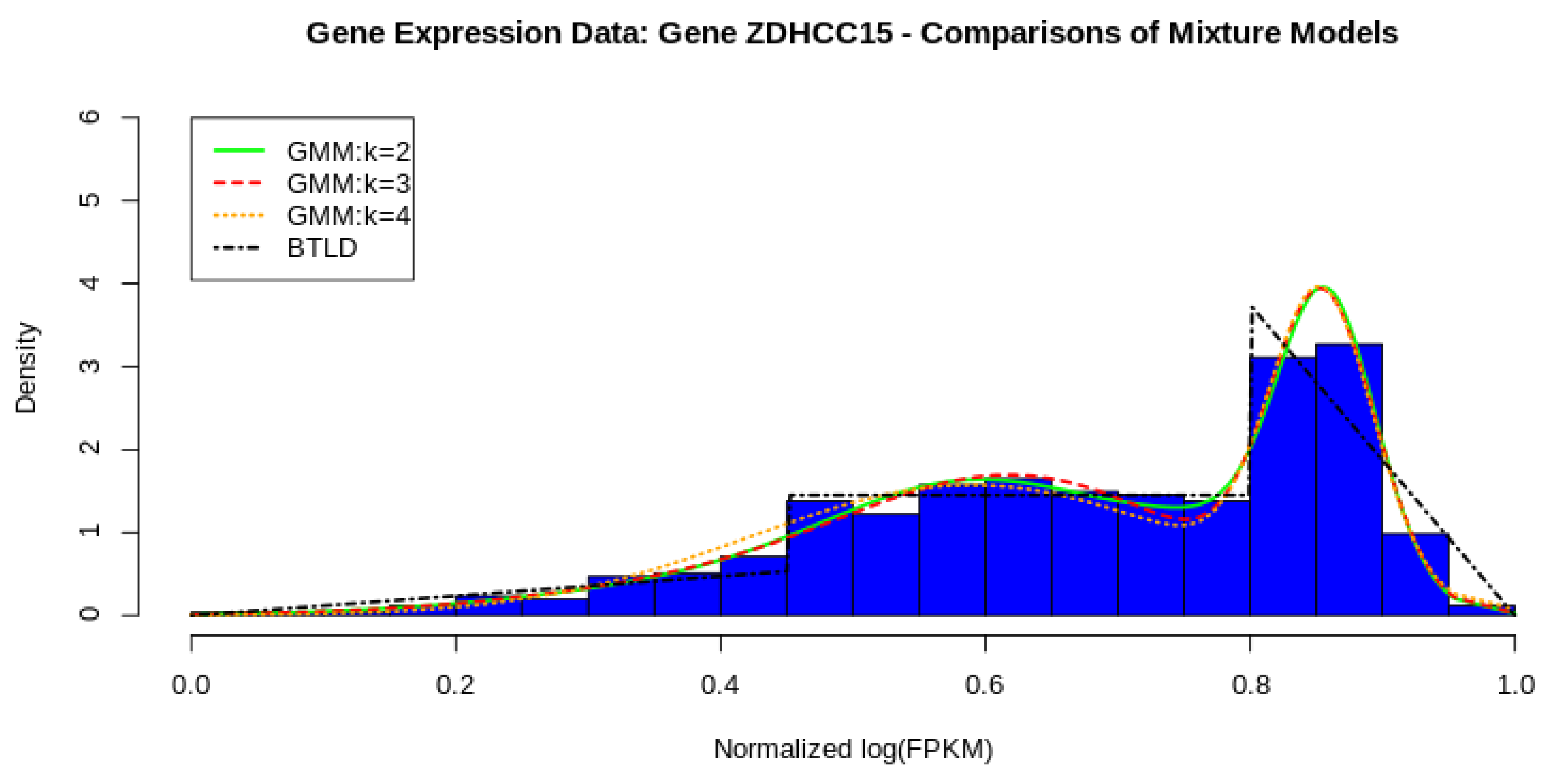
In Figure 8, we show the comparative fit of three GMMs against our parametric model, the bimodal triangular-linked distribution. From the figure, it seems evident that a two component mixture fits well to the data with three and four components not add much difference to the overall density fit. Furthermore, the three component and four component models do not converge in 1000 iterations which is troublesome, however, the two component model just fits in 38 iterations. In Table 1, we have tabulated the estimates used for $\widehat{\mathbf{\alpha }}$ and $\widehat{\mathbf{\theta }}$ for the BTL. These are calculated using the formulae provided by Equations (16) and (17).

Figure 8. BTL vs. GMM from 2 to 4 components.

Table 1. Estimates of BTL.

$\widehat{\mathit{\alpha }}$	$\widehat{\mathit{\theta }}$
0.53	0.45
2.95	0.85

If we compare to the fit of the BTL, we find that it has a very good fit. Using the Cramér–von Mises and the Kolmogorov–Smirnov tests, we find that the we do not reject the null hypothesis comfortably, even with the penalty on the CVM for sample estimated parameters (shown in Table 2). In Table 3, it an be seen that we also do not reject the null hypothesis for the KS and CVM tests. To get to more distinctive quantitative results, we look a the AIC and BIC scores in Table 4, where according to these relativistic metrics, the GMM outperforms the BTL as a density model. Furthermore, we visually illustrate the goodness of fit comparisons with the plots in Figure 9, showing a PP-plot and an ECDF plot of the two models, BTL and GMM.

Table 2. KS and CVM testing with the CDF of the BTL.

BTL	Test Statistic	p-Value
${\omega }^2$	0.48498	0.632
d	0.046772	0.2164

Table 3. KS and CVM testing using a pseudo-CDF for the GMM.

GMM	Test Statistic	p-Value
${\omega }^2$	0.82751	0.1233
d	0.024848	0.9124

Table 4. AIC and BIC scores.

	AIC	BIC
GMM	−437.7647	−425.0615
BTL	−376.8566	−368.3878

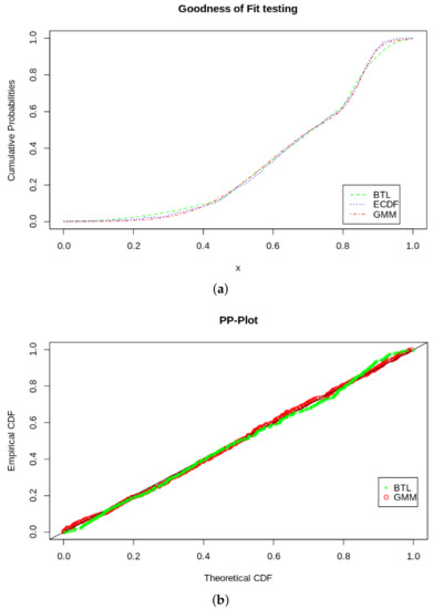
Figure 9. GOF tests. (a) ECDF, BTL CDF and GMM pseudo-CDF. (b) PP-plot of BTL and GMM.

7. Conclusions

The curse of dimensionality is a problem for all models. Working in higher dimensions complicates the modelling process. This is even more true for bimodal data since very few classical (i.e., normal, t) distributions that can accurately model bimodality in one dimension, let alone multiple dimensions. Most often, researchers turn to finite mixture models to capture bimodality. The use of finite mixture models does not provide five number summary statisics directly, bare useful tools such as the CDF which can used for prediction and confidence intervals and can be computationally expensive with k components in d dimensions. Furthermore, the choice of mixtures is most often a heuristic and in scenarios where the modes are close to each other, convergence of the EM algorithm is not guaranteed. Goodness-of-fit cannot be determined for mixture models and the only way to measure the model is by using machine learning metrics such as RMSE, accuracy, BIC and AIC.

In this paper, we introduce a simple mathematical model that addresses the issues with existing models for bimodality. The approach is as follows: The modes can be determined by identifying structural breaks in the empirical CDF. This is the only empirical information needed in order to fully specify the model estimates. We will investigate alternative approaches to determining the modes such as using KDEs as a proxy for mode estimate, MLEs and Methods of moments estimates.

In order to generalise to the multivariate case, we use a Gaussian copula. Copulas have found wide application in the field of actuarial modelling and investment management. We only take advantage of the dependance modelling of copulas to build the multivariate distribution as a fully fledged mathematical form of a multivariate distribution can necessitate a PhD to develop. A simulation of the multivariate distribution was illustrated and a comparison to a multivariate Gaussian mixture model was shown. An application in gene expression data of the univariate BTL vs. a GMM is shown. Finally, a package called btld was constructed from the workings of this paper.

Further research includes invesitgating the MVTL as a substitute for the compound Dirichlet distribution in modelling word rates. Furthermore, we can look to alternate copula structures to see how the multivariate distribution could change.

References

- Devore, J.L.; Berk, K.N. Modern Mathematical Statistics with Applications, 2nd ed.; Springer: New York, NY, USA, 2012; p. 835. [Google Scholar] [CrossRef]
- De Michele, C.; Accatino, F. Tree cover bimodality in savannas and forests emerging from the switching between two fire dynamic. PLoS ONE 2014, 9, e91195. [Google Scholar] [CrossRef] [PubMed] [Green Version]
- Giudici, P.; Figini, S. Applied Data Mining for Business and Industry, 2nd ed.; John Wiley & Sons: Chichester, UK, 2009. [Google Scholar] [CrossRef]
- Nguyen, H.D.; McLachlan, G. On approximations via convolution-defined mixture models. Commun. Stat.-Theory Methods 2019, 48, 3945–3955. [Google Scholar] [CrossRef]
- Shemyakin, A.; Kniazev, A. Introduction to Bayesian Estimation and Copula Models of Dependance; John Wiley & Sons: Hoboken, NJ, USA, 2017. [Google Scholar]
- Massey, F.J., Jr. The Kolmogorov–Smirnov test for goodness of fit. Am. Stat. Assoc. 1951, 46, 68–78. [Google Scholar] [CrossRef]
- Bonnini, S.; Corain, L.; Marozzi, M.; Salmaso, L. Nonparametric Hypothesis Testing: Rank and Permutation Methods with Applications in R; John Wiley & Sons: Chichester, UK, 2014. [Google Scholar]
- Taeger, D.; Kuhnt, S. Statistical Hypothesis Testing with SAS and R; John Wiley & Sons: Chichester, UK, 2014. [Google Scholar]
- Sheng, Y.; Soto, J.; Orlu Gul, M.; Cortina-Borja, M.; Tuleu, C.; Standing, J. New generalized poisson mixture model for bimodal count data with drug effect: An application to rodent brief-access taste aversion experiments. CPT Pharmacometr. Syst. Pharmacol. 2016, 5, 427–436. [Google Scholar] [CrossRef] [Green Version]
- Irace, Z.; Batatia, H. Bayesian spatiotemporal segmentation of combined PET-CT data using a bivariate Poisson mixture model. In Proceedings of the 2014 22nd European Signal Processing Conference (EUSIPCO), Lisbon, Portugal, 1–5 September 2014; pp. 2095–2099. [Google Scholar]
- Irace, Z. Modélisation Statistique et Segmentation d’Images TEP: Application à l’Hétérogénéité et au Suivi de Tumeurs. Ph.D. Thesis, Institut National Polytechnique de Toulouse, Toulouse, France, 2014. [Google Scholar]
- Justino, J.; Reis, C.; Fonseca, A.; de Souza, S.J.; Stransky, B. A new genome-wide method to identify genes with bimodal gene expression. bioRxiv 2020. [Google Scholar] [CrossRef]
- Sur, P.; Shmueli, G.; Bose, S.; Dubey, P. Modeling bimodal discrete data using Conway-Maxwell–Poisson mixture models. J. Bus. Econ. Stat. 2015, 33, 352–365. [Google Scholar] [CrossRef] [Green Version]
- Azzalini, A. A class of distributions which includes the normal ones. Scand. J. Stat. 1985, 12, 171–178. [Google Scholar]
- Elal-Olivero, D. Alpha-skew-normal distribution. Proyecciones 2010, 29, 224–240. [Google Scholar] [CrossRef] [Green Version]
- Shafiei, S.; Doostparast, M.; Jamalizadeh, A. The alpha–beta skew normal distribution: Properties and applications. Statistics 2016, 50, 338–349. [Google Scholar] [CrossRef]
- Balakrishnan, N. Skewed multivariate models related to hidden truncation and/or selective reporting-Discussion. Test 2002, 11, 7–54. [Google Scholar]
- Hazarika, P.J.; Shah, S.; Chakraborty, S. Balakrishnan alpha skew normal distribution: Properties and applications. arXiv 2019, arXiv:1906.07424. [Google Scholar] [CrossRef]
- Shah, S.; Hazarika, P.J.; Chakraborty, S.; Ali, M.M. The Balakrishnan-Alpha-Beta-Skew-Normal Distribution: Properties and Applications. Pak. J. Stat. Oper. Res. 2021, 17, 367–380. [Google Scholar] [CrossRef]
- Harandi, S.S.; Alamatsaz, M. Alpha–Skew–Laplace distribution. Stat. Probab. Lett. 2013, 83, 774–782. [Google Scholar] [CrossRef]
- Hazarika, P.J.; Chakraborty, S. Alpha-skew-logistic distribution. IOSR J. Math. 2014, 10, 36–46. [Google Scholar] [CrossRef]
- Shah, S.; Chakraborty, S.; Hazarika, P.J. A New One Parameter Bimodal Skew Logistic Distribution and its Applications. arXiv 2019, arXiv:1906.04125. [Google Scholar]
- Elal-Olivero, D.; Gómez, H.W.; Quintana, F.A. Bayesian modeling using a class of bimodal skew-elliptical distributions. J. Stat. Plan. Inference 2009, 139, 1484–1492. [Google Scholar] [CrossRef]
- Ma, Y.; Genton, M.G. Flexible class of skew-symmetric distributions. Scand. J. Stat. 2004, 31, 459–468. [Google Scholar] [CrossRef] [Green Version]
- Arnold, B.C.; Castillo, E.; Sarabia, J.M. Conditionally specified multivariate skewed distributions. Sankhyā Indian J. Stat. Ser. A 2002, 64, 206–226. [Google Scholar]
- Azzalini, A.; Capitanio, A. Distributions generated by perturbation of symmetry with emphasis on a multivariate skew t-distribution. J. R. Stat. Soc. Ser. B (Stat. Methodol.) 2003, 65, 367–389. [Google Scholar] [CrossRef]
- Ara, A.; Louzada, F. The multivariate alpha skew gaussian distribution. Bull. Braz. Math. Soc. New Ser. 2019, 50, 823–843. [Google Scholar] [CrossRef]
- Kim, H.J. On a class of two-piece skew-normal distributions. Statistics 2005, 39, 537–553. [Google Scholar] [CrossRef]
- Arellano-Valle, R.B.; Cortés, M.A.; Gómez, H.W. An extension of the epsilon-skew-normal distribution. Commun. Stat. Methods 2010, 39, 912–922. [Google Scholar] [CrossRef]
- Gómez, H.W.; Elal-Olivero, D.; Salinas, H.S.; Bolfarine, H. Bimodal extension based on the skew-normal distribution with application to pollen data. Environmetrics 2011, 22, 50–62. [Google Scholar] [CrossRef]
- Arnold, B.C.; Gómez, H.W.; Salinas, H.S. A doubly skewed normal distribution. Statistics 2015, 49, 842–858. [Google Scholar] [CrossRef]
- Rathie, P.N.; Silva, P.; Olinto, G. Applications of skew models using generalized logistic distribution. Axioms 2016, 5, 10. [Google Scholar] [CrossRef] [Green Version]
- Braga, A.d.S.; Cordeiro, G.M.; Ortega, E.M. A new skew-bimodal distribution with applications. Commun. Stat.-Theory Methods 2018, 47, 2950–2968. [Google Scholar] [CrossRef]
- Venegas, O.; Salinas, H.S.; Gallardo, D.I.; Bolfarine, H.; Gómez, H.W. Bimodality based on the generalized skew-normal distribution. J. Stat. Comput. Simul. 2018, 88, 156–181. [Google Scholar] [CrossRef]
- Shah, S.; Chakraborty, S.; Hazarika, P.J.; Ali, M.M. The Log-Balakrishnan-alpha-skew-normal distribution and its applications. Pak. J. Stat. Oper. Res. 2020, 16, 109–117. [Google Scholar] [CrossRef]
- Gómez-Déniz, E.; Pérez-Rodríguez, J.V.; Reyes, J.; Gómez, H.W. A Bimodal Discrete Shifted Poisson Distribution. A Case Study of Tourists’ Length of Stay. Symmetry 2020, 12, 442. [Google Scholar] [CrossRef] [Green Version]
- Wei, Z.; Peng, T.; Zhou, X. The Alpha-Beta-Gamma Skew Normal Distribution and Its Application. Open J. Stat. 2020, 10, 1057–1071. [Google Scholar] [CrossRef]
- Lin, T.I.; Lee, J.C.; Yen, S.Y. Finite mixture modelling using the skew normal distribution. Stat. Sin. 2007, 17, 909–927. [Google Scholar]
- Lin, T.I.; Lee, J.C.; Hsieh, W.J. Robust mixture modeling using the skew t distribution. Stat. Comput. 2007, 17, 81–92. [Google Scholar] [CrossRef]
- Kotz, S.; van Dorp, J.R. Chapter 1: The Triangular Distribution. In Beyond Beta, Other Continuous Families of Distributions with Bounded Support and Applications; World Scientific Press: Singapore, 2004; pp. 1–32. [Google Scholar] [CrossRef] [Green Version]
- Devroye, L. General Principles in Random Variate Generation. In Non-Uniform Random Variate Generation; Springer: New York, NY, USA, 1986; pp. 27–82. [Google Scholar] [CrossRef]
- Nelsen, R.B. An Introduction to Copulas; Springer Science & Business Media: New York, NY, USA, 2007. [Google Scholar]
- Sklar, A. Fonctions de répartition à n dimensions et leurs marge. Inst. Stat. L’Université Paris 1959, 8, 229–231. [Google Scholar]
- Haugh, M. IEOR E4602: Quantitative Risk Management and IEOR E4703: Monte-Carlo Simulation. In Quantitative Risk Management; Columbia University: New York, NY, USA, 2016; Volume 1. [Google Scholar] [CrossRef]
- Panjer, H.H. Operational Risk: Modeling Analytics; John Wiley & Sons: Hoboken, NJ, USA, 2006; Volume 620. [Google Scholar]
- Robert, C.; Casella, G. Introducing Monte Carlo methods with R. In Use R, 1st ed.; Springer: New York, NY, USA, 2010. [Google Scholar]
- Bishop, C. Pattern Recognition and Machine Learning. In Information Science and Statistics; Springer: Berlin/Heidelberg, Germany, 2006. [Google Scholar]
- R Core Team. R: A Language and Environment for Statistical Computing; R Foundation for Statistical Computing: Vienna, Austria, 2021. [Google Scholar]
- Benaglia, T.; Chauveau, D.; Hunter, D.R.; Young, D. mixtools: An R Package for Analyzing Finite Mixture Models. J. Stat. Softw. 2009, 32, 1–29. [Google Scholar] [CrossRef] [Green Version]
- Hofert, M.; Kojadinovic, I.; Maechler, M.; Yan, J. copula: Multivariate Dependence with Copulas. R Package Version 1.0-1. 2020. Available online: https://CRAN.R-project.org/package=copula (accessed on 2 February 2022).
- Iovleff, S.; Bathia, P. MixAll: Clustering and Classification Using Model-Based Mixture Models. 2019. Available online: https://cran.r-project.org/web/packages/MixAll/MixAll.pdf (accessed on 9 March 2022).
Publisher’s Note: MDPI stays neutral with regard to jurisdictional claims in published maps and institutional affiliations. |
© 2022 by the authors. Licensee MDPI, Basel, Switzerland. This article is an open access article distributed under the terms and conditions of the Creative Commons Attribution (CC BY) license (https://creativecommons.org/licenses/by/4.0/).