Analysis and Control of Malware Mutation Model in Wireless Rechargeable Sensor Network with Charging Delay

Abstract

In wireless rechargeable sensors (WRSNs), the system is vulnerable to be attacked by malware. Because of the distributed network structure of WRSNs, the malware attack has great influence on the security system of WRSNs. With the variability in malware, the problem of decryption and coding errors will lead to the malware mutating. In this paper, there are two problems to be solved, including the malware mutation and the charging delay in WRSNs. The malware mutation state and the low-energy state are introduced. Firstly, three different equilibrium solutions of the mutation model are given. Then, the local stability is proven by the characteristic equation, and the system will be stabilized at different equilibrium solutions when the base reproductive number is different. With the condition of charging delay, the bifurcation phenomenon is investigated by using the Hopf bifurcation theory. Furthermore, to improve the security of WRSNs and decrease the control cost, the Pontryagin’s Maximum principle is applied to obtain an optimal control scheme under mutation and charging delay. Finally, the numerical simulation is applied by Matlab to confirm this model. The simulation results show that the mutation malware can be controlled when the delay is less than the maximum threshold.

1. Introduction

With the development of various network applications, there are many network security issues for networks [1,2,3,4]. Thus, the security of wireless sensor network (WSN) is a hot topic [5,6,7]. Many authors have studied WSNs from different aspects. A WSN is a distributed network structure. It has a great number of sensor nodes connected by a common wireless channel. Thus, it is applied in many fields, such as the military, environmental monitoring, medical treatment, disaster management, automotive applications, and so on [8,9]. However, WSN is constrained by limited resource, processing speed, and battery life. Because of the deployment of the nodes, it is hard to create a complicated safeguard ability for a WSN. It is also easy to lead to information transmission failure or even network paralysis when the WSN is attacked by malware. Therefore, it is urgent and significant to take measures to ensure accuracy and efficiency in WSN.

More and more scholars have studied the propagation of malware. At first, Kephart et al. [10,11] studied the propagation of the virus by incorporating concepts of epidemic dynamics. Since then, this method has opened a new way to solve the security problems of networks. Liu et al. [12] studied the malware propagation on complex networks which follow the power-law degree distribution. A SEIR model is proposed by Zhu et al. [13], and the authors analyzed the threshold, time delay, and global stability of a rumor spreading on social networks. Then, authors [14,15] also studied the spread of rumors in complex networks. Huang et al. [16] proposed spreading dynamics of social behaviors in multiplex networks. With the mathematical model, a number of researchers have made attempts using different models for investigating the malware disseminating dynamics in WSNs. When considering the spatial and temproal parameters, Khayam et al. [17] proposed a worm propagation model by using signal processing techniques in WSN. A worm propagation model in a WSN is proposed in Refs. [18,19], and the authors took into account the communication radius and the distributed density of the nodes. In [20], Ojha et al. also proposed an improved model which aggregates quarantine and vaccination techniques by Feng et al. Muthukrishnan et al. [21] established the node-based malware trace and patching model. They studied the topological structure and proposed an optimal control strategy. In Ref. [22], the authors proposed the SIR1R2 with secondary immunity to analyze the feature of malware propagation in WSNs. In Ref. [18], a mathematical equation is presented as follows:

$$\left\{\begin{array}{c}\frac{{\displaystyle \mathrm{d}S}}{{\displaystyle \mathrm{d}t}}=\mu N-\xi SI-(\mu +\omega )S+ϵR\hfill \\ \\ \frac{{\displaystyle \mathrm{d}I}}{{\displaystyle \mathrm{d}t}}=\xi SI-(\mu +\gamma )I\hfill \\ \\ \frac{{\displaystyle \mathrm{d}R}}{{\displaystyle \mathrm{d}t}}=\omega S+\gamma I-(\mu +ϵ)R\hfill \\ \end{array}\right.$$

(1)

where, S, I, and R are the state nodes. They mean the numbers of the susceptible, the infected, and the recovered nodes, respectively. As shown in

Table 1. Notation.

N	The number of all nodes in the WSN
$\mu$	The proportion of birth and death sensor nodes
$\xi$	The proportion of susceptible nodes becoming infected nodes
$\omega$	The proportion of susceptible nodes becoming recovered nodes
$\gamma$	The proportion of infected nodes becoming recovered nodes
$ϵ$	The proportion of recovered nodes becoming susceptible nodes

, the parameters are explained.

To study the malware spread specifically, other factors are taken into account in the mawlare spreading model, including time delay, virus mutation, the battery life, etc. Because of the battery capacity limitations, many scholars also pay attention to rechargeable WSN schemes [23,24,25] to solve the battery life problem. Li et al. [26] proposed an energy-efficient patching strategy to solve the problems of virus attacks and energy constraints. Liu et al. [27,28] considered the impact of pulse charging and charging delay on the system. Keshri et al. [29] proposed an SEIR model with two time delays (including the period exposed and the period of temporary immunity). They studied the effect of delay in the WSN during multiple attacks. In Ref. [30], the authors proposed the propagation of a worm model with three delays and analyzed the influence of multiple delays on a system. For these time delay models [31,32,33], the authors investigated the condition of Hopf bifurcation. However, the energy constraint is the most important problem to be solved for all delay problems. It is necessary to study the low-energy state and the influence of charging delay on a WSN’s efficiency. Liu et al. [34] proposed the malware propagation model when considering the low-energy state. They revealed the relationship between the charging rate and the basic reproductive number. However, they did not analyze the effect of a charging delay in WRSNs.

At the moment, it is worth noting that virus mutation [35] means that a virus is likely to convert to another virus when transmitting the virus on networks. In most networks, the malware mutation is real [36]. The condition of mutation needs to be considered, but few people have studied dynamic models of malware mutation. Li et al. [37,38] proposed an epidemic model with virus mutation and considered the virus mutation during transmission. Afterwards, they considered the virus’s spontaneous variation, and they only established a delay model with virus mutation; they did not analyze the effect of delay on the mutation model. Hao [39] proposed the virus variation model on complex networks. They mainly analyzed the stability. In Ref. [40], the authors proposed a SIVR model to investigate the dynamics of epidemic propogation with virus mutation on complex networks, and they only discussed different epidemic immunization strategies to control the propagation of viruses and their mutations. Regardless of mutation, there are some control methods, including dissemination of security patches or recovery in Ref. [41]. Zhang et al. [42] considered the control strategy of the SIQRS model and provided three measures of vaccination, quarantine, and treatment. Zhu et al. [43] established an optimal control model with delay, and four different control strategies were investigated. Many excellent works have also been described in Refs. [44,45,46]. Chen et al. [47] considered the virus mutation with drug resistance and proposed an SIVRS epidemic spreading model on scale-free networks. They analyzed the mutation under heterogeneous networks. The model has only one reproductive number, and the model could not reflect the influence of the variation and infection node well. Liu et al. [48,49] analyzed the propagation of malware with virus mutation in wireless sensor networks. They merely studied the stability and control. Based on the above survey, there are many problems with mutation models. However, few people have studied charging delays and mutation models simultaneously. Moreover, the problem of optimal control needs to be solved.

In this paper, a new model is proposed to consider charging delay and mutation. A complex SIIRL model is proposed in WSN. S, $I_1$, $I_2$, R, and L mean the numbers of the susceptible, the infected, the mutation malware, the recovered, and the low-energy nodes, respectively. Our contributions are as follows:

1.

For existing mutation models, the WSN has an energy constraint. As a solution, charging needs to be completed within a certain period of time. To address this problem, the mutation model with charging delay is proposed to analyse the process of spreading malware. The effect of charging delay on mutation model is also analyzed.

2.

Through the analysis of the mutation model with charging delay, two different basic reproductive numbers, $R_1$ and $R_2$, are obtained. Then, the locally asymptotically stability is proven. Moreover, the bifurcation phenomenon and periodic oscillation of the mutation model are analyzed.

3.

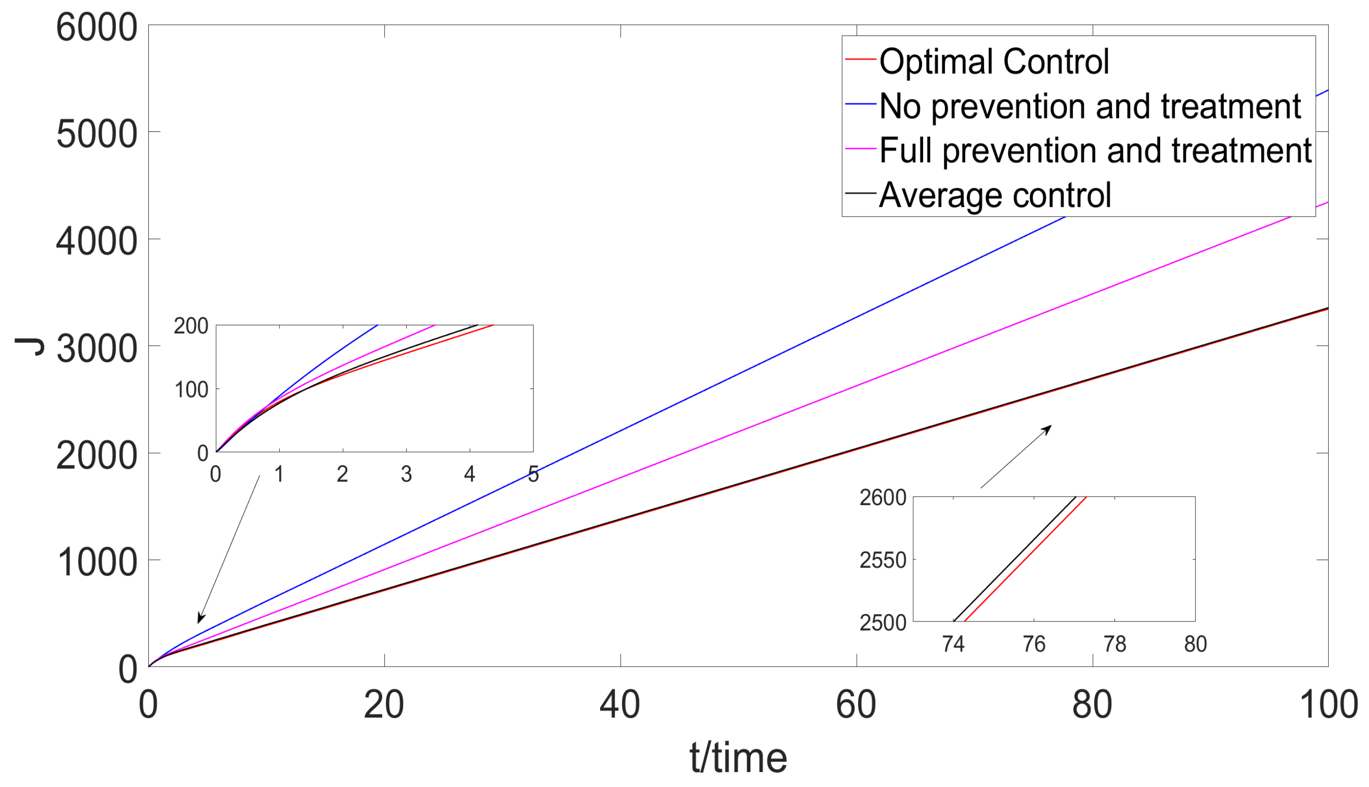
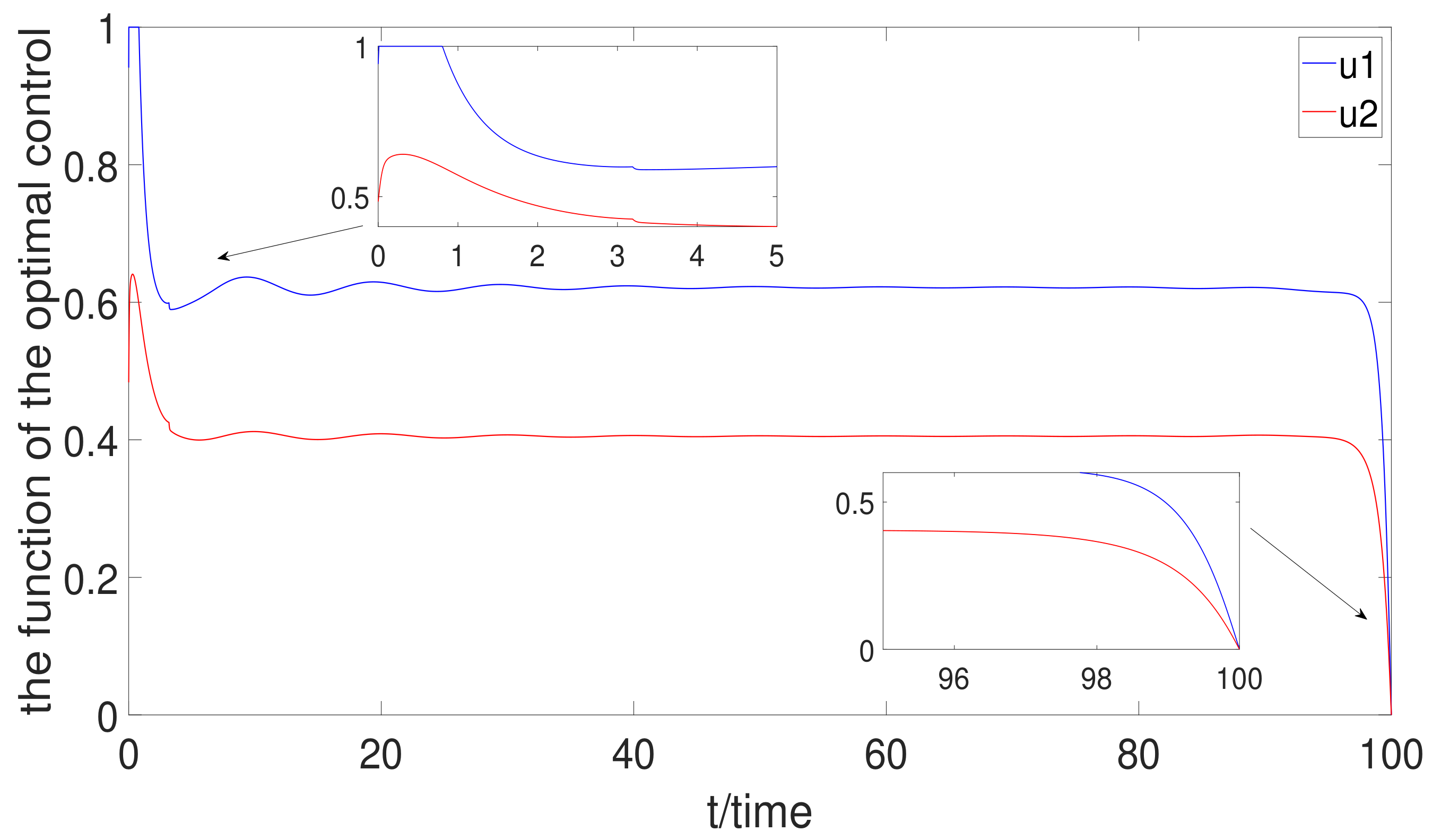
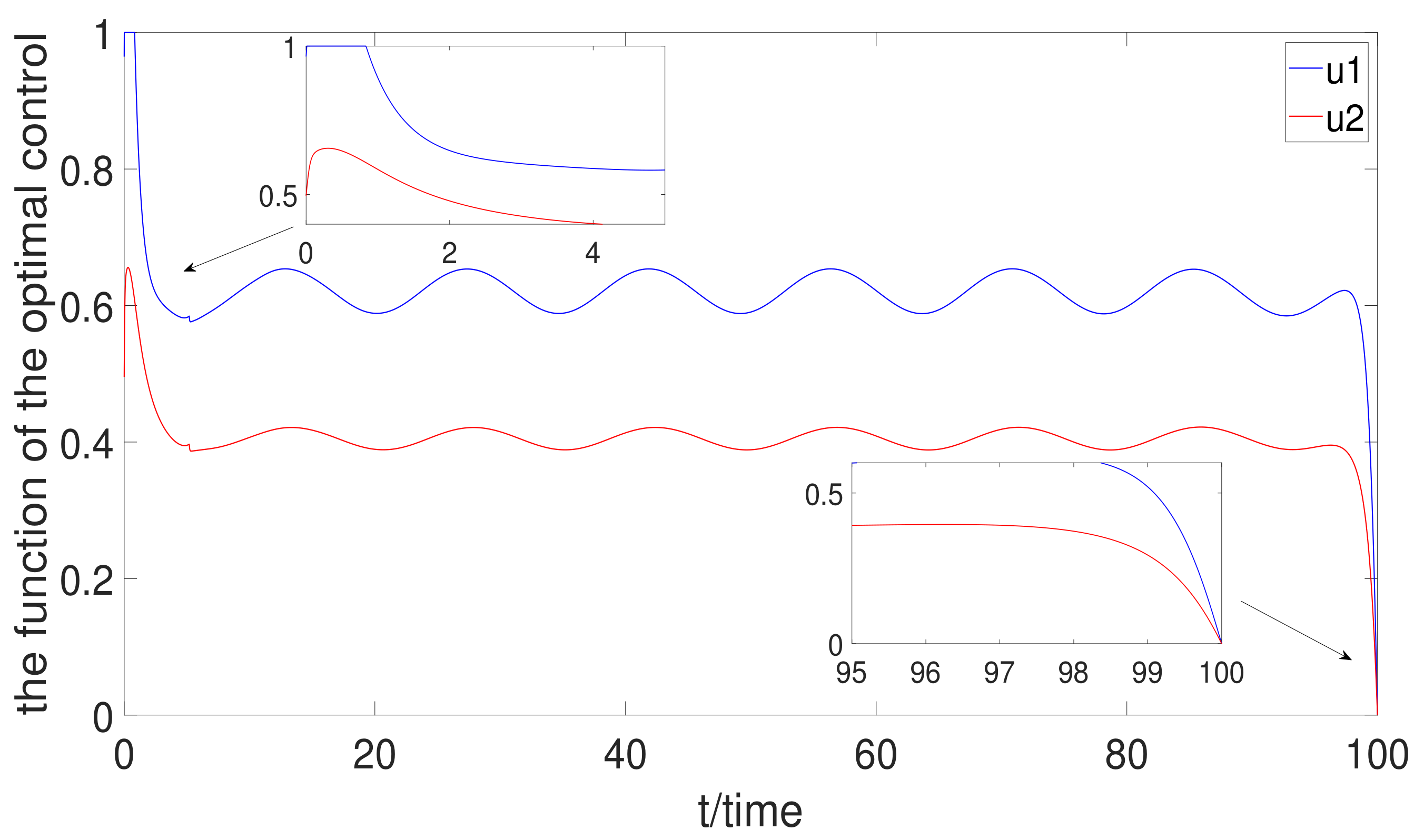
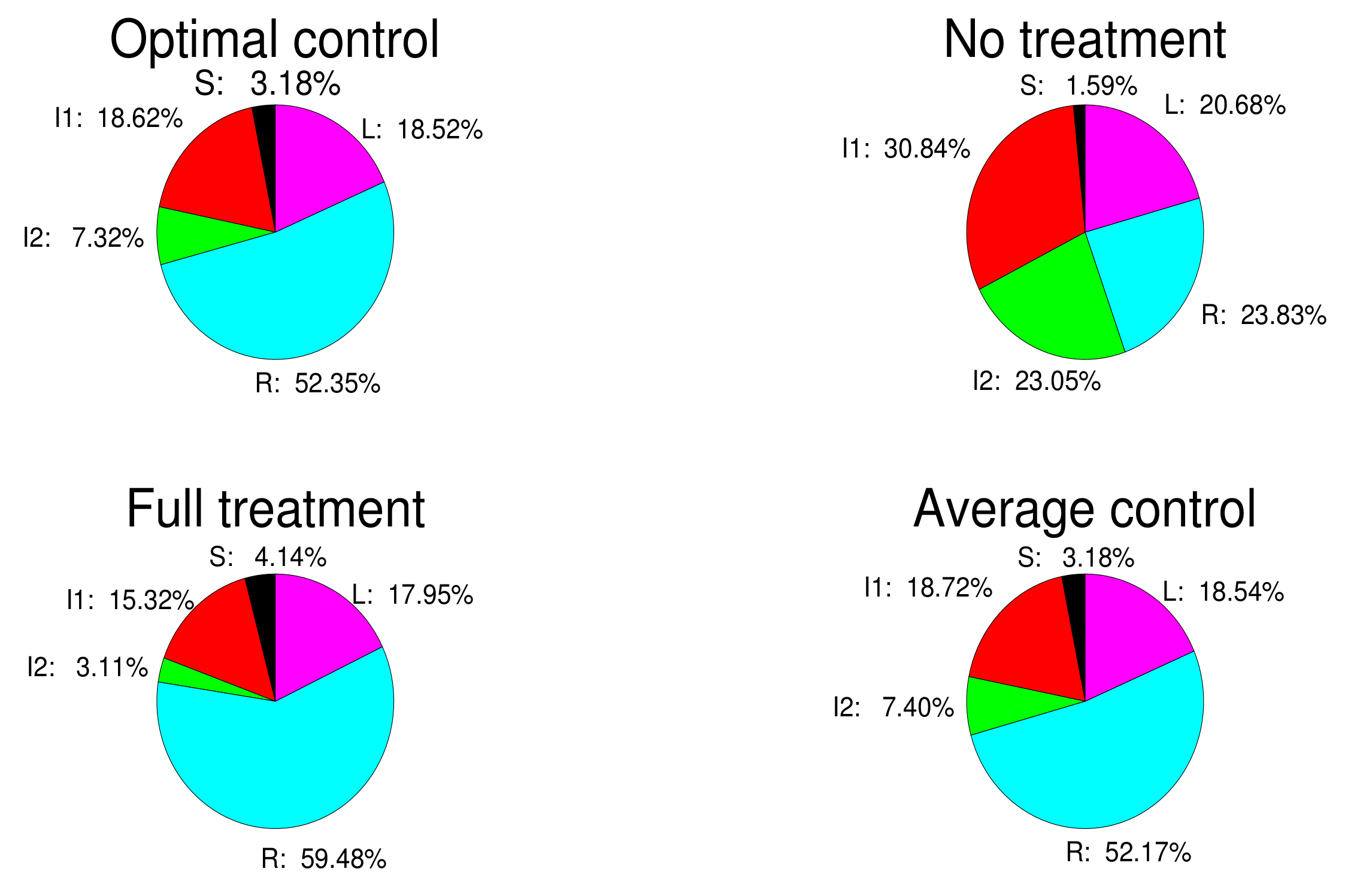
Based on the mutation model with charging delay, the optimal charging delay control strategy is discussed. According to the Pontryagin’s Maximun Principle, the optimal variable $u^{*}\left(t\right)$ can be derived. It is found that the charging delay has great influence on optimal control. Meanwhile, no treatment control, average control, and full treatment are also analyzed. By comparison with the three control methods, the optimal control is the best control method of them.

The follow of this paper is organized as follows. In Section 2, the SIIRL model is proposed. The mean-field equations are analyzed. In Section 3, the equilibrium points are calculated, and the local stability and the bifurcation phenomenon are investigated. In Section 4, the direction of Hopf bifurcation is analyzed. In Section 5, the charging delay control strategy is proposed for mutation malware spreading in WRSNs. In Section 6, some simulations are described to support the theoretical analysis. Finally, in Section 7, the conclusion of the model is described.

2. Modeling

In this section, the model of malware spreading is introduced. In general, the condition of normal and abnormal depends on if the sensors are infected or not. The normal working sensors are not infected by malware such as S and R. For example, the energy consumption of S is normal. R will be not be attacked. Thus, the energy consumption of R is normal. The abnormal working sensors are infected by malware such as $I_1$ and $I_2$. The nodes will consume a lot of energy when the sensors run the malware. The assumption is proposed that the conversion ratio of S or R to L is the same $c_1$ and the conversion ratio of $I_1$ or $I_2$ to L is the same $c_2$. As depicted above, the model of equation is given as follows:

$$\left\{\begin{array}{c}\frac{{\displaystyle \mathrm{d}S}}{{\displaystyle \mathrm{d}t}}=A-{\beta }_{1}S{I}_1-{\beta }_{2}S{I}_2-c_{1}S-dS+\alpha R\hfill \\ \\ \frac{{\displaystyle \mathrm{d}{I}_1}}{{\displaystyle \mathrm{d}t}}={\beta }_{1}S{I}_1-(c_2+d+\epsilon +{\gamma }_1)I_1\hfill \\ \\ \frac{{\displaystyle \mathrm{d}{I}_2}}{{\displaystyle \mathrm{d}t}}={\beta }_{2}S{I}_2-(c_2+d+{\gamma }_2)I_2+\epsilon I_1\hfill \\ \\ \frac{{\displaystyle \mathrm{d}R}}{{\displaystyle \mathrm{d}t}}={\gamma }_1{I}_1+{\gamma }_2{I}_2+\mu L(t-\tau )-(c_1+d+\alpha )R\hfill \\ \\ \frac{{\displaystyle \mathrm{d}L}}{{\displaystyle \mathrm{d}t}}=c_1(R+S)+c_2(I_2+I_1)-\mu L(t-\tau )-dL\hfill \end{array}\right.$$

(2)

According to Equation (2), A is the quantity of the injected nodes; ${\beta }_1$ is the conversion ratio of susceptible to infected; ${\beta }_2$ is the conversion ratio of the susceptible to virus mutation; $\epsilon$ is the conversion ratio of the infected to virus mutation; $c_1$ is the conversion ratio of the susceptible or recovered to low energy; $c_2$ is the conversion ratio of the infected or virus mutation to low energy; d is the conversion ratio of the sensor death; ${\gamma }_1$ is the conversion ratio of the infected to the recovered; ${\gamma }_2$ is the conversion ratio of the virus mutation to the recovered; $\mu$ is the conversion ratio of recovery from low energy; $\alpha$ is the failure ratio of recovery; and $\tau$ is the time delay.

3. Local Stability and Existence of Hopf Bifurcation

According to the system (2), the solutions of the system, including the disease-free equilibrium, the boundary equilibrium, and the endemic equilibrium, are given by:

$$\begin{array}{cc}\hfill S_0& =\frac{A(\alpha d+c_{1}d+\alpha \mu +d\mu +d^2)}{d(\alpha +c_1+d)(c_1+d+\mu )}\hfill \end{array}$$

(3)

$$\begin{array}{cc}\hfill \overline{S}& =\frac{c_2+{\gamma }_2+d}{{\beta }_2}\hfill \end{array}$$

(4)

$$\begin{array}{cc}\hfill S^{*}& =\frac{c_2+{\gamma }_1+d+\epsilon }{{\beta }_1}\hfill \end{array}$$

(5)

The disease-free equilibrium is $E_0(S_0,0,0,R_0,L_0)$. According to the next generation, the basic reproductive numbers can be calculated. The matrix is given by:

$$F=\left[\begin{array}{cc}{\beta }_1{S}_0& 0\\ 0& {\beta }_2{S}_0\end{array}\right]V=\left[\begin{array}{cc}{c}_2+d+{\gamma }_1+\epsilon & 0\\ -\epsilon & c_2+d+{\gamma }_2\end{array}\right]$$

(6)

Thus, the basic reproductive numbers are given by:

$$\begin{array}{cc}\hfill R_1& =\left(F{V}_1^{-1}\right)=\frac{{\beta }_1{S}_0}{c_2+d+{\gamma }_1+\epsilon }\hfill \\ \hfill \end{array}$$

(7)

$$\begin{array}{cc}\hfill R_2& =\left(F{V}_2^{-1}\right)=\frac{{\beta }_2{S}_0}{c_2+d+{\gamma }_2}\hfill \end{array}$$

(8)

If $R_1<1$ and $R_2<1$, the system has a disease-free equilibrium solution; if $R_2>1$ and $R_2>R_1$, the system has a disease-free equilibrium solution and a boundary equilibrium solution; if $R_1>1$ and $R_1>R_2$, the system has a disease-free equilibrium solution and an endemic equilibrium solution. The equilibrium is given as:

$$\begin{array}{cc}\hfill R^0& =\frac{A{c}_1\mu }{((\mu +d)(c_1+d)-c_1\mu )(c_1+d)}=\frac{A{c}_1\mu }{(\mu +c_1+d)(c_1+d)d}\hfill \end{array}$$

(9)

$$\begin{array}{cc}\hfill L^0& =\frac{(c_1+d)R^0}{\mu }=\frac{A{c}_1}{(\mu +d)(c_1+d)-c_1\mu }=\frac{A{c}_1}{(\mu +c_1+d)d}\hspace{1em}\hfill \\ \hfill \end{array}$$

(10)

$$\begin{array}{cc}\hfill \overline{I_2}& =\frac{c_1\overline{S}\mu \alpha (c_1+d+\alpha )}{[c_1{\gamma }_1+c_2(c_1+d+\alpha )]\mu \alpha +[\mu c_1-(\mu +d)(c_1+d+\alpha )]}\hfill \\ \hfill \end{array}$$

(11)

$$\begin{array}{cc}\hfill \overline{L}& =\frac{{\gamma }_2\overline{I_2}-(c_1+d+\alpha )\overline{R}}{\mu }\hspace{1em}\hspace{1em}\hspace{1em}\hspace{1em}\hspace{1em}\hspace{1em}\hspace{1em}\hspace{1em}\hspace{1em}\hspace{1em}\hspace{1em}\hspace{1em}\hspace{1em}\hspace{1em}\hspace{1em}\hfill \\ \hfill \end{array}$$

(12)

$$\begin{array}{cc}\hfill \overline{R}& =\frac{A-{\beta }_2\overline{S}\overline{I_2}-(c_1+d)\overline{S}}{\alpha }\hfill \\ \hfill \end{array}$$

(13)

$$\begin{array}{cc}\hfill I_1^{*}& =\frac{I_2^{*}[(c_2+d+{\gamma }_1)-{\gamma }_2{S}^{*}]}{\epsilon }\hfill \\ \hfill \end{array}$$

(14)

$$\begin{array}{cc}\hfill \hspace{1em}\hspace{1em}\hspace{1em}\hspace{1em}\hspace{1em}\hspace{1em}{I}_2^{*}& =\frac{c_1{S}^{*}\alpha \mu -(A-(c_1+d)S^{*})c_1\mu +(A-(c_1+d)S^{*})(c_1+d+\alpha )(\mu +d)\epsilon \mu \alpha }{\alpha \mu [(Q_1+Q_2+Q_3)-Q_4]}\hfill \end{array}$$

(15)

$$\begin{array}{cc}\hfill \hspace{1em}\hspace{1em}\hspace{1em}\hspace{1em}{R}^{*}& =\frac{\left({\beta }_1{S}^{*}((c_2+d+{\gamma }_1)-{\beta }_2{S}^{*})\right)I_2^{*}-(A-(c_1+d)S^{*})\epsilon }{\epsilon \alpha }\hfill \\ \hfill \end{array}$$

(16)

$$\begin{array}{cc}\hfill \hspace{1em}\hspace{1em}\hspace{1em}{L}^{*}& =\frac{(Q_4-Q_3)I_2^{*}-\left((A-(c_1+d)S^{*})(c_1+d+\alpha )\epsilon \right)}{\alpha \mu \epsilon }\hfill \end{array}$$

(17)

where,

$$\begin{array}{cc}\hfill Q_1& =\mu \alpha c_2((c_2+d+{\gamma }_2)-{\beta }_2{S}^{*}+\epsilon )\hfill \\ \hfill \end{array}$$

(18)

$$\begin{array}{cc}\hfill \hspace{1em}{Q}_2& =c_1{\beta }_1{S}^{*}\mu ((c_2+d+{\gamma }_1)-{\beta }_2{S}^{*})+\epsilon \mu {\beta }_2{S}^{*}{c}_1\hfill \\ \hfill \end{array}$$

(19)

$$\begin{array}{cc}\hfill Q_3& =\alpha {\gamma }_1{\beta }_1{S}^{*}((c_2+d+{\gamma }_1)-{\beta }_2{S}^{*})+{\gamma }_2\epsilon \alpha \hfill \\ \hfill \end{array}$$

(20)

$$\begin{array}{cc}\hfill \hspace{1em}\hspace{1em}\hspace{1em}\hspace{1em}\hspace{1em}\hspace{1em}\hspace{1em}{Q}_4& =({\beta }_1{S}^{*}((c_2+d+{\gamma }_1)+{\beta }_2{S}^{*})+{\beta }_2{S}^{*}\epsilon )(c_1+d+\alpha )(\mu +d)\hfill \end{array}$$

(21)

The characteristic matrix is given as:

$$X=\left[\begin{array}{ccccc}\lambda +a_1& {\beta }_{1}S& {\beta }_{2}S& -\alpha & 0\\ -{\beta }_1{I}_1& \lambda -a_1& 0& 0& 0\\ -{\beta }_2{I}_2& -\epsilon & \lambda -a_3& 0& 0\\ 0& -{\gamma }_1& -{\gamma }_2& \lambda +a_4& -\mu e^{-\lambda \tau }\\ -c_1& -c_2& -c_2& -c_1& \lambda +d+\mu e^{-\lambda \tau }\end{array}\right]$$

(22)

where

$$\left\{\begin{array}{c}{a}_1=\lambda +{\beta }_1{I}_1+{\beta }_2{I}_2+(c_1+d)\hfill \\ \\ a_2={\beta }_{1}S-(c_2+d+{\gamma }_2+\epsilon )\hfill \\ \\ a_3={\beta }_{2}S-(c_2+d+{\gamma }_2)\hfill \\ \\ a_4=c_1+d+\alpha \hfill \end{array}\right.\left\{\begin{array}{c}{b}_1={\beta }_1{I}_1{\beta }_{1}S\hfill \\ \\ b_2={\beta }_2{I}_2{\beta }_{2}S\hfill \\ \\ b_3={\beta }_1{I}_1{\beta }_{2}S\hfill \\ \\ b_4=c_1+d\hfill \end{array}\right.$$

(23)

The characteristic equation is given by:

$$f\left(\lambda \right)=A_5{\lambda }^5+A_4{\lambda }^4+A_3{\lambda }^3+A_2{\lambda }^2+A_1\lambda +A_0+B{e}^{-\lambda \tau }$$

(24)

where $A_5=1$, and the others are given by:

$$\begin{array}{cc}\hfill A_4=& a_1-a_2-a_3+a_4+d\hfill \end{array}$$

(25)

$$\begin{array}{cc}\hfill A_3=& -(-b_1-b_2+a_1{a}_2+a_1{a}_3-a_1{a}_4-a_2{a}_3+a_2{a}_4+a_3{a}_4-(a_1-a_2-a_3+a_4)d\hfill \\ \hfill A_2=& a_1{a}_2{a}_3-a_1{a}_2{a}_4-a_1{a}_3{a}_4+a_2{a}_3{a}_4-a_1{a}_{2}d-a_1{a}_{3}d+a_1{a}_{4}d+a_2{a}_{3}d-a_2{a}_{4}d-a_3{a}_{4}d-b_1{a}_3+b_1{a}_4-b_2{a}_2\hfill \end{array}$$

(26)

$$\begin{array}{cc}& +b_2{a}_4+b_{1}d+b_{2}d+b_3\epsilon +\alpha {\beta }_1{I}_1{\gamma }_1+\alpha {\beta }_2{I}_2{\gamma }_2\hfill \\ \hfill A_1=& a_1{a}_2{a}_3{a}_4+a_1{a}_2{a}_{3}d-a_1{a}_2{a}_{4}d-a_1{a}_3{a}_{4}d+a_2{a}_3{a}_{4}d-a_3{a}_4{b}_1-a_2{a}_4{b}_2-a_3{b}_{1}d+a_4{b}_{1}d-a_2{b}_{2}d+a_4{b}_{2}d+a_4{b}_3\epsilon \hfill \end{array}$$

(27)

$$\begin{array}{cc}& +b_{3}d\epsilon -a_3\alpha {\beta }_1{I}_1{\gamma }_1-a_2\alpha {\beta }_2{I}_2{\gamma }_2+\alpha {\beta }_1{I}_1{\gamma }_{1}d+\alpha {\beta }_2{I}_2{\gamma }_{2}d+\alpha \epsilon {\beta }_1{I}_1{\gamma }_2\hfill \end{array}$$

(28)

$$\begin{array}{cc}\hfill A_0=& -a_3{a}_4{b}_{1}d-a_2{a}_4{b}_{2}d+a_1{a}_2{a}_3{a}_{4}d+a_4{b}_{3}d\epsilon -a_3\alpha {\beta }_1{I}_1{\gamma }_{1}d-a_2\alpha {\beta }_2{I}_2{\gamma }_{2}d+\alpha \epsilon {\beta }_1{I}_1{\gamma }_{2}d\hfill \\ \hfill B=& \mu {\lambda }^4+(a_1\mu -a_2\mu -a_3\mu +a_4\mu -b_4){\lambda }^3+(b_1\mu +b_2\mu -a_1{a}_2\mu -a_1{a}_3\mu +a_1{a}_4\mu +a_2{a}_3\mu -a_2{a}_4\mu -a_3{a}_4\mu -a_1{b}_4\hfill \\ & +a_2{b}_4+a_3{b}_4+\alpha b_4){\lambda }^2+(a_1{a}_2{a}_3\mu -a_1{a}_2{a}_4\mu -a_1{a}_3{a}_4\mu +a_2{a}_3{a}_4\mu -a_1{a}_2{b}_4+a_1{a}_3{b}_4-a_2{a}_3{b}_4-a_3{b}_1\mu +a_4{b}_1\mu \hfill \\ & -a_2{b}_2\mu +a_4{b}_2\mu -b_1{b}_4-b_2{b}_4+b_3\epsilon \mu -a_2\alpha b_4-a_3\alpha b_4+\alpha {\beta }_1{I}_1{c}_2\mu +\alpha {\beta }_2{I}_2{c}_2\mu +\alpha {\beta }_1{I}_1{\gamma }_1\mu +\alpha {\beta }_2{\gamma }_2\mu )\lambda +(a_1{a}_2{a}_3{a}_4\mu \hfill \end{array}$$

(29)

$$\begin{array}{cc}& -a_1{a}_2{a}_3{b}_4-a_3{a}_4{b}_1\mu -a_2{a}_4{b}_2\mu +a_3{b}_1{b}_4+a_2{b}_2{b}_4+a_4{b}_3\epsilon \mu -b_3{b}_4\epsilon )\hfill \end{array}$$

(30)

Theorem 1.

If $R_1<1$ and $R_2<1$, $E_0(S_0,0,0,R_0,L_0)$ is locally asymptotically stable when $\tau =0$.

Proof. 

If $\tau =0$, Equation (24) can be depicted:

$$\begin{array}{cc}\hfill f\left(\lambda \right)=& {\lambda }^5+A_4{\lambda }^4+A_3{\lambda }^3+A_2{\lambda }^2+A_1\lambda +A_0+B{e}^{-\lambda \tau }\hfill \\ \hfill =& {\lambda }^5+(A_4+\mu ){\lambda }^4+(A_3+(a_1\mu -a_2\mu -a_3\mu +a_4\mu -b_4)){\lambda }^3+(A_2+(b_1\mu +b_2\mu -a_1{a}_2\mu -a_1{a}_3\mu +a_1{a}_4\mu +a_2{a}_3\mu \hfill \\ & -a_2{a}_4\mu -a_3{a}_4\mu -a_1{b}_4+a_2{b}_4+a_3{b}_4+\alpha b_4){\lambda }^2+(A_1+(a_1{a}_2{a}_3\mu -a_1{a}_2{a}_4\mu -a_1{a}_3{a}_4\mu +a_2{a}_3{a}_4\mu -a_1{a}_2{b}_4+a_1{a}_3{b}_4\hfill \\ & -a_2{a}_3{b}_4-a_3{b}_1\mu +a_4{b}_1\mu -a_2{b}_2\mu +a_4{b}_2\mu -b_1{b}_4-b_2{b}_4+b_3\epsilon \mu -\alpha a_2{b}_4-\alpha a_3{b}_4+\alpha {\beta }_1{I}_1{c}_2\mu +\alpha {\beta }_2{I}_2{c}_2\mu +\alpha {\beta }_1{I}_1{\gamma }_1\mu \hfill \\ & +\alpha {\beta }_2{I}_2{\gamma }_2\mu \left)\right)\lambda +(A_0+(a_1{a}_2{a}_3{a}_4\mu -a_1{a}_2{a}_3{b}_4-a_3{a}_4{b}_1\mu -a_2{a}_4{b}_2\mu +a_3{b}_1{b}_4+a_2{b}_2{b}_4+a_4{b}_3\epsilon \mu -b_3{b}_4\epsilon +a_2{a}_3\alpha b_4\hfill \\ & -a_3\alpha {\beta }_1{I}_1{c}_2\mu -a_2\alpha {\beta }_2{I}_2{c}_2\mu -a_3\alpha {\beta }_1{I}_1{\gamma }_1\mu -a_2\alpha {\beta }_2{I}_2{\gamma }_2\mu +\alpha {\beta }_1{I}_1\epsilon c_2\mu +\alpha {\beta }_1{I}_1{\gamma }_2\epsilon \mu \left)\right)\hfill \end{array}$$

(31)

Thus, through putting $E_0$ into Equation (22), we can obtain $b_1=b_2=b_3=0$. Equation (31) can be given as follows:

$$\begin{array}{cc}\hfill f\left(\lambda \right)=& {\lambda }^5+(A_{41}+\mu ){\lambda }^4+(A_{31}+(a_1\mu -a_2\mu -a_3\mu +a_4\mu -b_4)){\lambda }^3+(A_{21}+(-a_1{a}_2\mu -a_1{a}_3\mu +a_1{a}_4\mu +a_2{a}_3\mu -a_2{a}_4\mu \hfill \\ & -a_3{a}_4\mu -a_1{b}_4+a_2{b}_4+a_{3}b+\alpha b_4\left)\right){\lambda }^2+(A_{11}+(a_1{a}_2{a}_3\mu -a_1{a}_2{a}_4\mu -a_1{a}_3{a}_4\mu +a_2{a}_3{a}_4\mu -a_1{a}_2{b}_4+a_1{a}_3{b}_4-a_2{a}_3{b}_4\hfill \\ & -\alpha a_2{b}_4-\alpha a_3{b}_4+\alpha {\beta }_1{I}_1{c}_2\mu +\alpha {\beta }_2{I}_2{c}_2\mu +\alpha {\beta }_1{I}_1{\gamma }_1\mu +\alpha {\beta }_2{I}_2{\gamma }_2\mu \left)\right)\lambda +(A_{01}+(a_1{a}_2{a}_3{a}_4\mu -a_1{a}_2{a}_3{b}_4+\alpha a_2{a}_3{b}_4\hfill \\ & -\alpha a_3{\beta }_1{I}_1{c}_2\mu -a_2\alpha {\beta }_2{I}_2{c}_2\mu +a_3\alpha {\beta }_1{I}_1{\gamma }_1\mu -a_2\alpha {\beta }_2{I}_2{\gamma }_2\mu +\alpha {\beta }_1{I}_1\epsilon c_2\mu +\alpha {\beta }_1{I}_1{\gamma }_2\epsilon \mu \left)\right)\hfill \end{array}$$

(32)

where

$$\begin{array}{cc}\hfill n_5=& A_{51}=1n_4=A_{41}+\mu n_3=A_{31}+(a_1\mu -a_2\mu -a_3\mu +a_4\mu -b_4)\hfill \\ \hfill n_2=& A_{21}+(-a_1{a}_2\mu -a_1{a}_3\mu +a_1{a}_4\mu +a_2{a}_3\mu +a_2{a}_3\mu -a_2{a}_4\mu -a_3{a}_4\mu -a_1{b}_4+a_2{b}_4\hfill \\ & +a_3{b}_4+\alpha b_4)\hfill \\ \hfill n_1=& A_{11}+(a_1{a}_2{a}_3\mu -a_1{a}_2{a}_4\mu -a_1{a}_3{a}_4\mu +a_2{a}_3{a}_4\mu -a_1{a}_2{b}_4+a_1{a}_3{b}_4-a_2{a}_3{b}_4-\alpha a_2{b}_4\hfill \\ & -\alpha a_3{b}_4+\alpha {\beta }_1{I}_1{c}_2\mu +\alpha {\beta }_2{I}_2{c}_2\mu +\alpha {\beta }_1{I}_1{\gamma }_1\mu +\alpha {\beta }_2{I}_2{\gamma }_2\mu )\hfill \\ \hfill n_0=& A_{01}+(a_1{a}_2{a}_3{a}_4\mu -a_1{a}_2{a}_3{b}_4+\alpha a_2{a}_3{b}_4-\alpha a_3{\beta }_1{I}_1{c}_2\mu -\alpha a_2{\beta }_2{I}_2{c}_2\mu -\alpha a_3{\beta }_1{I}_1{\gamma }_1\mu \hfill \\ & -\alpha a_2{\beta }_2{I}_2{\gamma }_2\mu +\alpha {\beta }_1{I}_1\epsilon c_2\mu +\alpha {\beta }_1{I}_1{\gamma }_2\epsilon \mu )\hfill \end{array}$$

(33)

$\hspace{1em}\hspace{1em}\hspace{1em}\hspace{1em}\hspace{1em}\hspace{1em}\hspace{1em}\hspace{1em}\hspace{1em}{n}_5=1>0,{\Delta }_1=\left|n_4\right|=n_4$

$${\Delta }_2=\left|\begin{array}{cc}{n}_4& 1\\ n_2& n_3\end{array}\right|=n_4{n}_3-n_2$$

$${\Delta }_3=\left|\begin{array}{ccc}{n}_4& 1& 0\\ n_2& n_3& n_4\\ n_0& n_1& n_2\end{array}\right|=n_4(n_3{n}_2-n_4{n}_1)-(n_2^2-n_4{n}_0)$$

$${\Delta }_4=\left|\begin{array}{cccc}{n}_4& 1& 0& 0\\ n_2& n_3& n_4& 1\\ n_0& n_1& n_2& n_3\\ 0& 0& n_0& n_1\end{array}\right|=n_3{n}_1-n_3{n}_2{n}_0+n_5{n}_0(n_4{n}_1-n_5{n}_0)$$

$${\Delta }_5=\left|\begin{array}{ccccc}{n}_4& 1& 0& 0& 0\\ n_2& n_3& n_4& 1& 0\\ n_0& n_1& n_2& n_3& n_4\\ 0& 0& n_0& n_1& n_2\\ 0& 0& 0& 0& n_0\end{array}\right|=n_0{\Delta }_4$$

(34)

□

Assumption A1.

For the system (2), when $\tau =0$, if the conditions ($R_1<1$, $R_2<1$, ${\Delta }_1>0,$${\Delta }_2>0,$${\Delta }_3>0,{\Delta }_4>0,{\Delta }_5>0$), $E_0(S_0,0,0,R_0,L_0)$ is locally asymptotically stable in accordance with the Routh–Hurwitz criterion.

Theorem 2.

If $R_1<1$ and $R_2>1$, $\overline{E}(\overline{S},0,\overline{I},\overline{R},\overline{L})$ is locally asymptotically stable when $\tau =0$.

Proof. 

If $\tau =0$, according to Equation (22), $b_1=b_3=0$ and $a_3=0$ can be obtained. Equation (24) can be given as follows:

$$\begin{array}{cc}\hfill f\left(\lambda \right)=& {\lambda }^5+A_4{\lambda }^4+A_3{\lambda }^3+A_2{\lambda }^2+A_1\lambda +A_0+B{e}^{-\lambda \tau }\hfill \\ \hfill =& {\lambda }^5+(A_4+\mu ){\lambda }^4+(A_3-(a_2\mu -a_1\mu -a_4\mu +b_4)){\lambda }^3+(A_2+(b_2\mu -a_1{a}_2\mu +a_1{a}_4\mu -a_2{a}_4\mu -a_1{b}_4+a_2{b}_4+\alpha b_4){\lambda }^2\hfill \\ & +(A_1-(a_1{a}_2{a}_4\mu +a_1{a}_2{b}_4+a_2{b}_4\alpha -{\beta }_2{I}_2{c}_2\mu \alpha -{\beta }_2{I}_2{\gamma }_2\mu \alpha +a_2{b}_2\mu -a_4{b}_2\mu +b_2{b}_4))\lambda +(A_0-(a_4{b}_2\mu -a_2{b}_2{b}_4\hfill \\ & +a_2\alpha {\beta }_2{I}_2{c}_2\mu +a_2\alpha {\beta }_2{I}_2{\gamma }_2\mu \left)\right)\hfill \end{array}$$

(35)

Similarly, according to the Routh–Hurwitz criterion, $\overline{E}(\overline{S},0,\overline{I},\overline{R},\overline{L})$ is locally asymptotically stable. □

Case 1. if $\tau >0$,

$$\begin{array}{cc}\hfill B_4=& \mu B_3=(a_1\mu -a_2\mu +a_4\mu -b_4)\hfill \\ \hfill B_2=& (b_2\mu -a_1{a}_2\mu +a_1{a}_4\mu -a_2{a}_4\mu -a_1{b}_4+a_2{b}_4+\alpha b_4)\hfill \\ \hfill B_1=& (-a_1{a}_2{a}_4\mu -a_1{a}_2{b}_4-a_2{b}_2\mu +a_4{b}_2\mu -b_2{b}_4-\alpha a_2{b}_4+\alpha {\beta }_2{I}_2{c}_2\mu +\alpha {\beta }_2{I}_2{\gamma }_2\mu )\hfill \\ \hfill B_0=& (-a_2{a}_4{b}_2\mu +a_2{b}_2{b}_4-\alpha a_2{\beta }_2{I}_2{c}_2\mu -\alpha a_2{\beta }_2{I}_2{\gamma }_2\mu )\hfill \end{array}$$

(36)

The characteristic equation can be obtained:

$$f\left(\lambda \right)={\lambda }^5+A_{42}{\lambda }^4+A_{32}{\lambda }^3+A_{22}{\lambda }^2+A_{12}\lambda +A_{02}+(B_4{\lambda }^4+B_3{\lambda }^3+B_2{\lambda }^2+B_1\lambda +B_0)e^{-\lambda \tau }$$

(37)

If the root of Equation (37) is $\lambda =i\omega$, Equation (37) can be depicted as follows:

$$\begin{array}{cc}\hfill f\left(i\omega \right)=& {\left(i\omega \right)}^5+A_{42}{\left(i\omega \right)}^4+A_{32}{\left(i\omega \right)}^3+A_{22}{\left(i\omega \right)}^2+A_{12}\left(i\omega \right)+A_{02}+(B_4{\left(i\omega \right)}^4+B_3{\left(i\omega \right)}^3+B_2{\left(i\omega \right)}^2+B_1\left(i\omega \right)+B_0)e^{-i\omega \tau }\hfill \end{array}$$

(38)

Hence, the imaginary component and real component can be given as:

$$\left\{\begin{array}{c}(A_{42}{\omega }^4-A_{22}{\omega }^2+A_{02})+(B_4{\omega }^4-B_2{\omega }^2+B_0)cos\left(\omega \tau \right)-(B_3{\omega }^3-B_1\omega )sin\left(\omega \tau \right)=0\hfill \\ \\ (i{\omega }^5-A_{32}i{\omega }^3+A_{12}i\omega )-(B_{3}i{\omega }^3-B_{1}i\omega )cos\left(\omega \tau \right)-(B_4{\omega }^4-B_2{\omega }^2+B_0)isin\left(\omega \tau \right)=0\hfill \end{array}\right.$$

⇒

$$\left\{\begin{array}{c}{A}_{42}{\omega }^4-A_{22}{\omega }^2+A_{02}=(B_3{\omega }^3-B_1\omega )sin\left(\omega \tau \right)-(B_4{\omega }^4-B_2{\omega }^2+B_0)cos\left(\omega \tau \right)\mathrm{①}\hfill \\ \\ -{\omega }^5+A_{32}{\omega }^3-A_{12}\omega =(-B_3{\omega }^3+B_1\omega )cos\left(\omega \tau \right)-(B_4{\omega }^4-B_2{\omega }^2+B_0)sin\left(\omega \tau \right)\mathrm{②}\hfill \end{array}\right.$$

(39)

Thus, $({\mathrm{①}}^1+{\mathrm{②}}^2)$ can be obtained as follows:

$${\omega }^{10}+H_{81}{\omega }^8+H_{61}{\omega }^6+H_{41}{\omega }^4+H_{21}{\omega }^2+H_{01}=0$$

(40)

With

$$\left\{\begin{array}{c}{H}_{81}=A_{42}^2-2A_{32}-B_4^2\hfill \\ \\ H_{61}=A_{32}^2-2A_{12}-2A_{22}{A}_{42}-(B_3^2-2B_4{B}_2)\hfill \\ \\ H_{41}=A_{22}^2+2A_{02}{A}_{42}-2A_{12}{A}_{32}-(2B_4{B}_0+B_2^2-2B_1{B}_3)\hfill \\ \\ H_{21}=A_{12}^2-2A_{12}{A}_{22}-(B_1^2-2B_2{B}_0)\hfill \\ \\ H_{01}=A_{02}^2-B_0^2\hfill \end{array}\right.$$

(41)

Let $V={\omega }^2$. Equation (40) is given by:

$$V^5+H_{81}{V}^4+H_{61}{V}^3+H_{41}{V}^2+H_{21}V+H_{01}=0$$

(42)

Obviously, if $H_{01}<0$, Equation (42) has one positive root at least. Thus, the assumption can be obtained as follows.

Assumption A2.

We assume Equation (42) has five solutions and each solution has a different τ.

According to Equation (39), ① of Equation (39) can be obtained as follows:

$$\begin{array}{cc}\hfill \frac{(A_{42}{\omega }^4-A_{22}{\omega }^2+A_{02})(B_4{\omega }^4-B_2{\omega }^2+B_0)}{B_3{\omega }^3-B_1\omega }=& (B_4{\omega }^4-B_2{\omega }^2+B_0)sin\left(\omega \tau \right)-\frac{(B_4{\omega }^4-B_2{\omega }^2+B_0)}{B_3{\omega }^3-B_1\omega }cos\left(\omega \tau \right)\hfill \end{array}$$

(43)

Hence, Equation (39) of $(\mathrm{①}+\mathrm{②})$ is given by:

$$\begin{array}{cc}\hfill & (A_{42}{\omega }^4-A_{22}{\omega }^2+A_{02})(B_4{\omega }^4-B_2{\omega }^2+B_{02})+(-{\omega }^5+A_{32}{\omega }^3-A_{12}\omega )(B_3{\omega }^3-B_1\omega )\hfill \\ & ={(-{(B_4{\omega }^4-B_2{\omega }^2+B_0)}^2-{\left(B_3\omega \right)}^3-B_1\omega )}^2)cos\left(\omega \tau \right)\hfill \end{array}$$

(44)

From Equation (44), the value of $\tau$ can be obtained:

$$\begin{array}{cc}\hfill P=& (A_{42}{\omega }^4-A_{22}{\omega }^2+A_{02})(B_4{\omega }^4-B_2{\omega }^2+B_0)+(-{\omega }^5+A_{32}{\omega }^3-A_{12}\omega )(B_3{\omega }^3-B_1\omega )\hfill \\ \hfill Q=& -{(B_4{\omega }^4-B_2{\omega }^2+B_0)}^2-{(B_3{\omega }^3-B_0\omega )}^2\hfill \end{array}$$

(45)

where

$$\begin{array}{c}\hfill \tau =\left[arccos\left(\frac{P}{Q}\right)+2n\pi \right]\frac{1}{\omega },n=1,2,3\dots \dots \end{array}$$

(46)

The positive root of Equation (46) obtains the solution of $\tau$. When $\omega ={\omega }_{10}$, ${\tau }_{10}$ can be obtained:

$${\tau }_{10}=min\left\{{\tau }_{1i}^0\right\},i=1,2\dots \dots 5$$

(47)

Then Equation (37) has a purely imaginary roots $\pm i{\omega }_{10}$. When $\omega ={\omega }_{10}$, differentiating both side of Equation (37) can be obtained:

$$\frac{{\displaystyle \mathrm{d}\lambda }}{{\displaystyle \mathrm{d}\tau }}=\frac{\lambda (B_4{\lambda }^4+B_3{\lambda }^3+B_2{\lambda }^2+B_1\lambda +B_0)e^{-\lambda \tau }}{z1+z2-z3}$$

(48)

With

$$\begin{array}{cc}\hfill z1=& (5{\lambda }^4+4A_{42}{\lambda }^3+3A_{32}{\lambda }^2+2A_{22}\lambda +A_{12})\hfill \\ \hfill z2=& (4B_4{\lambda }^3+3B_3{\lambda }^2+2B_2\lambda +B_1)e^{-\lambda \tau }\hfill \\ \hfill z3=& \tau (B_4{\lambda }^4+B_3{\lambda }^3+B_2{\lambda }^2+B_1\lambda +B_0)e^{-\lambda \tau }\hfill \end{array}$$

(49)

where $\tau ={\tau }_{10}$. Equation (48) is given by:

$$\begin{array}{cc}\hfill {\left[\frac{{\displaystyle \mathrm{d}\lambda }}{{\displaystyle \mathrm{d}{\tau }_{10}}}\right]}^{-1}=& \frac{5{\lambda }^4+4A_{42}{\lambda }^3+3A_{32}{\lambda }^2+2A_{22}\lambda +A_{12}}{-\lambda ({\lambda }^5+A_{42}{\lambda }^4+A_{32}{\lambda }^3+A_{22}{\lambda }^2+A_{12}\lambda +A_{02}}\hfill \\ & +\frac{4B_4{\lambda }^3+3B_3{\lambda }^2+2B_2\lambda +B_1}{\lambda (B_4{\lambda }^4+B_3{\lambda }^3+B_2{\lambda }^2+B_1\lambda +B_0)}-\frac{{\tau }_{10}}{\lambda }\hfill \end{array}$$

(50)

Thus, $Re{\left[\frac{{\displaystyle \mathrm{d}\lambda }}{{\displaystyle \mathrm{d}{\tau }_{10}}}\right]}^{-1}\ne 0$ is a transversality condition of the Hopf bifurcation theorem. The results can be given as:

Theorem 3.

For the system (2), if $R_1<1,R_2>1$ and $\tau \in [0,{\tau }_{10})$, $\overline{E}(\overline{S},0,\overline{I},\overline{R},\overline{L})$ is locally asymptotically stable, and if $\tau \ge {\tau }_{10}$, a Hopf bifurcation occurs at $\overline{E}(\overline{S},0,\overline{I},\overline{R},\overline{L})$.

Theorem 4.

If $R_1>1$ and $R_1>R_2$, $E^{*}(S^{*},I_1^{*},I_2^{*},R^{*},L^{*})$ is locally asymptotically stable when $\tau =0$.

Proof. 

If $\tau =0$, Equation (24) can be given by:

$$\begin{array}{cc}\hfill f\left(\lambda \right)=& {\lambda }^5+A_{43}{\lambda }^4+A_{33}{\lambda }^3+A_{23}{\lambda }^2+A_{13}\lambda +A_{03}+\mu {\lambda }^4+(a_1\mu -a_2\mu -a_3\mu +a_4\mu -b_4){\lambda }^3+(b_1\mu +b_2\mu -a_1{a}_2\mu -a_1{a}_3\mu \hfill \\ & +a_1{a}_4\mu +a_2{a}_3\mu -a_2{a}_4\mu -a_3{a}_4\mu -a_1{b}_4+a_2{b}_4+a_3{b}_4+\alpha b_4){\lambda }^2+(a_1{a}_2{a}_3\mu -a_1{a}_2{a}_4\mu -a_1{a}_3{a}_4\mu +a_2{a}_3{a}_4\mu -a_1{a}_2{b}_4\hfill \\ & +a_1{a}_3{b}_4-a_2{a}_3{b}_4-a_3{b}_1\mu +a_4{b}_1\mu -a_2{b}_2\mu +a_4{b}_2\mu -b_1{b}_4-b_2{b}_4+b_3\mu \epsilon -\alpha a_2{b}_4-\alpha a_3{b}_4+\alpha {\beta }_1{I}_1{c}_2\mu +\alpha {\beta }_2{I}_2{c}_2\mu \hfill \\ & +\alpha {\beta }_1{I}_1{\gamma }_1\mu +\alpha {\beta }_2{I}_2{\gamma }_2\mu )\lambda +(a_1{a}_2{a}_3{a}_4\mu -a_1{a}_2{a}_3{b}_4-a_3{a}_4{b}_1\mu -a_2{a}_4{b}_2\mu +a_3{b}_1{b}_4+a_2{b}_2{b}_4+\alpha a_2{a}_3{b}_4-\alpha a_3{\beta }_1{I}_1{c}_2\mu \hfill \\ & -\alpha a_2{\beta }_2{I}_2{c}_2\mu -\alpha a_3{\beta }_1{I}_1{\gamma }_1\mu -\alpha a_2{\beta }_2{I}_2{\gamma }_2\mu +\alpha {\beta }_1{I}_1\epsilon c_2\mu +\alpha {\beta }_1{I}_1{\gamma }_2\epsilon \mu +a_4{b}_3\epsilon \mu -b_3{b}_4\mu )\hfill \end{array}$$

(51)

where

$$\begin{array}{cc}\hfill p_5=& 1\hfill \\ \hfill p_4=& A_{43}+\mu \hfill \\ \hfill p_3=& A_{33}+(a_1\mu -a_2\mu -a_3\mu +a_4\mu -b_4)\hfill \\ \hfill p_2=& A_{23}+(b_1\mu +b_2\mu -a_1{a}_2\mu -a_1{a}_3\mu +a_1{a}_4\mu +a_2{a}_3\mu -a_2{a}_4\mu -a_3{a}_4\mu -a_1{b}_4+a_2{b}_4+a_3{b}_4\hfill \\ & +\alpha b_4)\hfill \\ \hfill p_1=& A_{13}+(a_1{a}_2{a}_3\mu -a_1{a}_2{a}_4\mu -a_1{a}_3{a}_4\mu +a_2{a}_3{a}_4\mu -a_1{a}_2{b}_4+a_1{a}_3{b}_4-a_2{a}_3{b}_4-a_3{b}_1\mu +a_4{b}_1\mu \hfill \\ & -a_2{b}_2\mu +a_4{b}_2\mu -b_1{b}_4-b_2{b}_4+b_3\mu \epsilon -\alpha a_2{b}_4-\alpha a_3{b}_4+\alpha {\beta }_1{I}_1{c}_2\mu +\alpha {\beta }_2{I}_2{c}_2\mu +\alpha {\beta }_1{I}_1{\gamma }_1\mu \hfill \\ & +\alpha {\beta }_2{I}_2{\gamma }_2\mu )\hfill \\ \hfill p_0=& A_{03}+(a_1{a}_2{a}_3{a}_4\mu -a_1{a}_2{a}_3{b}_4-a_3{a}_4{b}_1\mu -a_2{a}_4{b}_2\mu +a_3{b}_1{b}_4+a_2{b}_2{b}_4+a_4{b}_3\epsilon \mu -b_3{b}_4\mu \hfill \\ & -\alpha a_3{\beta }_1{I}_1{c}_2\mu -\alpha a_2{\beta }_2{I}_2{c}_2\mu -\alpha a_3{\beta }_1{I}_1{\gamma }_1\mu -\alpha a_2{\beta }_2{I}_2{\gamma }_2\mu +\alpha {\beta }_1{I}_1\epsilon c_2\mu +\alpha {\beta }_1{I}_1{\gamma }_2\epsilon \mu )\hfill \end{array}$$

(52)

Then,

$${\Delta }_1=\left|p_4\right|=p_4$$

$${\Delta }_2=\left|\begin{array}{cc}{p}_4& 1\\ p_2& p_3\end{array}\right|=p_4{p}_3-p_2$$

$${\Delta }_3=\left|\begin{array}{ccc}{p}_4& 1& 0\\ p_2& p_3& p_4\\ p_0& p_1& p_2\end{array}\right|=p_4(p_3{p}_2-p_4{p}_1)-(p_2^2-p_4{p}_0)$$

$${\Delta }_4=\left|\begin{array}{cccc}{p}_4& 1& 0& 0\\ p_2& p_3& p_4& 1\\ p_0& p_1& p_2& p_3\\ 0& 0& p_0& p_1\end{array}\right|=p_3{p}_1-p_3{p}_2{p}_0+p_5{p}_0(p_4{p}_1-p_5{p}_0)$$

$${\Delta }_5=\left|\begin{array}{ccccc}{p}_4& 1& 0& 0& 0\\ p_2& p_3& p_4& 1& 0\\ p_0& p_1& p_2& p_3& p_4\\ 0& 0& p_0& p_1& p_2\\ 0& 0& 0& 0& p_0\end{array}\right|=p_0{\Delta }_4$$

(53)

□

Assumption A3.

For the system (2), when $\tau =0$, if the conditions ($R_1>1$, $R_1>R_2$, ${\Delta }_1>0,{\Delta }_2>0,{\Delta }_3>0,{\Delta }_4>0,{\Delta }_5>0$), $E^{*}(S^{*},I_1^{*},I_2^{*},R^{*},L^{*})$ is local asymptotically stable in accordance with the Routh–Hurwitz criterion.

Case 2. If $\tau >0$, Equation (24) can be depicted:

$$f\left(\lambda \right)={\lambda }^5+A_{43}{\lambda }^4+A_{33}{\lambda }^3+A_{23}{\lambda }^2+A_{13}\lambda +A_{03}+(C_4{\lambda }^4+C_3{\lambda }^3+C_2{\lambda }^2+C_1\lambda +C_0)e^{-\lambda \tau }$$

(54)

With

$$\begin{array}{cc}\hfill C_4=& \mu \hfill \\ \hfill C_3=& (a_1\mu -a_2\mu -a_3\mu +a_4\mu -b_4)\hfill \\ \hfill C_2=& ((b_1\mu +b_2\mu -a_1{a}_2\mu -a_1{a}_3\mu +a_1{a}_4\mu +a_2{a}_3\mu -a_2{a}_4\mu -a_3{a}_4\mu -a_1{b}_4+a_2{b}_4+a_3{b}_4+\alpha b_4)\hfill \\ \hfill C_1=& (a_1{a}_2{a}_3\mu -a_1{a}_2{a}_4\mu -a_1{a}_3{a}_4\mu +a_2{a}_3{a}_4\mu -a_1{a}_2{b}_4+a_1{a}_3{b}_4-a_2{a}_3{b}_4-a_3{b}_1\mu +a_4{b}_1\mu \hfill \\ & -a_2{b}_2\mu +a_4{b}_2\mu -b_1{b}_4-b_2{b}_4+b_3\mu \epsilon -\alpha a_2{b}_4-\alpha a_3{b}_4+\alpha {\beta }_1{I}_1{c}_2\mu +\alpha {\beta }_2{I}_2{c}_2\mu +\alpha {\beta }_1{I}_1{\gamma }_1\mu \hfill \\ & +\alpha {\beta }_2{I}_2{\gamma }_2\mu )\hfill \\ \hfill C_0=& (a_1{a}_2{a}_3{a}_4\mu -a_1{a}_2{a}_3{b}_4-a_3{a}_4{b}_1\mu -a_2{a}_4{b}_1\mu +a_3{b}_1{b}_4+a_2{b}_2{b}_4+a_4{b}_3\epsilon \mu -b_3{b}_4\mu +\alpha a_2{a}_3{b}_4\hfill \\ & -\alpha a_3{\beta }_1{I}_1{c}_2\mu -\alpha a_2{\beta }_2{I}_2{c}_2\mu -\alpha a_3{\beta }_1{I}_1{\gamma }_1\mu -\alpha a_2{\beta }_2{I}_2{\gamma }_2\mu +\alpha {\beta }_1{I}_1\epsilon c_2\mu +\alpha {\beta }_1{I}_1{\gamma }_2\epsilon \mu )\hfill \end{array}$$

(55)

Suppose that $\lambda =i\sigma$, the real part and imaginary part is given as:

$$\begin{array}{c}\hfill \left\{\begin{array}{c}{A}_{43}{\sigma }^4-A_{23}{\sigma }^2+A_{03}+(C_4{\sigma }^4-C_2{\sigma }^2+C_0)cos\sigma \tau +(-C_3{\sigma }^3+C_1\sigma )sin\sigma \tau \mathrm{③}\hfill \\ \\ {\sigma }^5-A_{33}{\sigma }^3+A_{13}\sigma +(-C_3{\sigma }^3+C_1\sigma )cos\sigma \tau -(C_4{\sigma }^4-C_2{\sigma }^2+C_0)sin\sigma \tau \mathrm{④}\hfill \end{array}\right.\end{array}$$

(56)

Let $J={\sigma }^2$. $({\mathrm{③}}^2+{\mathrm{④}}^2)$ can be expressed:

$$J^5+K_{81}{J}^4+K_{61}{J}^3+K_{41}{J}^2+K_{21}J+K_{01}=0$$

(57)

With

$$\begin{array}{c}\hfill \left\{\begin{array}{c}{K}_{81}=A_{43}^2-2A_{33}-C_4^2\hfill \\ \\ K_{61}=2A_{13}-2A_{43}{A}_{23}+A_{33}^2-C_3^2+2C_4{C}_2\hfill \\ \\ K_{41}=2A_{43}{A}_{03}+A_{23}^2-2A_{33}{A}_{13}+2C_3{C}_1-2C_4{C}_0-C_0^2\hfill \\ \\ K_{21}=A_{13}^2-2A_{23}{A}_{03}-C_1^2+2C_2{C}_0\hfill \\ \\ K_{01}=A_{03}^2-C_0^2\hfill \end{array}\right.\end{array}$$

(58)

Assumption A4.

If $R_1>1$ and $R_1>R_2$, Equation (57) has five solutions, and each solution has a different τ.

④ of Equation (56) can be depicted as follows:

$$\begin{array}{cc}\hfill \frac{(A_{43}{\sigma }^4-A_{23}{\sigma }^2+A_{03})(C_4{\sigma }^4-C_2{\sigma }^2+C_0)}{C_3{\sigma }^3-C_1\sigma }=& (C_4{\sigma }^4-C_2{\sigma }^2+C_0)sin\left(\sigma \tau \right)\hfill \\ & -\frac{{(C_4{\sigma }^4-C_2{\sigma }^2+C_0)}^2}{C_3{\sigma }^3-C_1\sigma }cos\left(\sigma \tau \right)\hfill \end{array}$$

(59)

Thus, Equation (59) can be given by:

$$\begin{array}{cc}\hfill (& A_{43}{\sigma }^4-A_{23}{\sigma }^2+A_{03})(C_4{\sigma }^4-C_2{\sigma }^2+C_0)-({\sigma }^5-A_{33}{\sigma }^3+A_{13}\sigma )(C_3{\sigma }^3-C_1\sigma )\hfill \\ & =-\left({(C_4{\sigma }^4-C_2{\sigma }^2+C_0)}^{+}{(C_3{\sigma }^3-C_1\sigma )}^2\right)cos\left(\sigma \tau \right)\hfill \end{array}$$

(60)

From Equation (60), $\tau$ can be obtained:

$$\begin{array}{c}\hfill \tau =\left[arccos\frac{(A_{43}{\sigma }^4-A_{23}{\sigma }^2+A_{03})(C_4{\sigma }^4-C_2{\sigma }^2+C_0)-({\sigma }^5-A_{33}{\sigma }^3+A_{13}\sigma )}{-{(C_4{\sigma }^4-C_2{\sigma }^2+C_0)}^2-{(C_3{\sigma }^3-C_1\sigma )}^2)}+2n\pi \right]\frac{1}{\sigma }\\ \hfill n=1,2,3\dots \dots \end{array}$$

(61)

The positive root of Equation (60) can be solved for the solution of $\tau$. When $\sigma ={\sigma }_{10}$, the ${\tau }_{20}$ can be obtained:

$${\tau }_{20}=min\left\{{\tau }_{2i}^0\right\},i=1,2\dots \dots 5$$

(62)

Then, Equation (54) has the imaginary roots $\pm i{\sigma }_{10}$. When $\sigma ={\sigma }_{10}$, differentiating both side of Equation (54) can be obtained:

$$\frac{{\displaystyle \mathrm{d}\lambda }}{{\displaystyle \mathrm{d}\tau }}=\frac{\lambda (C_4{\lambda }^4+C_3{\lambda }^3+C_2{\lambda }^2+C_1\lambda +C_0)e^{-\lambda \tau }}{z4+z5-z6}$$

(63)

With

$$\begin{array}{cc}\hfill z4=& (5{\lambda }^4+4A_{43}{\lambda }^3+3A_{33}{\lambda }^2+2A_{23}\lambda +A_{13})\hfill \\ \hfill z5=& (4C_4{\lambda }^3+3C_3{\lambda }^2+2C_2\lambda +C_1)e^{-\lambda \tau }\hfill \\ \hfill z6=& \tau (C_4{\lambda }^4+C_3{\lambda }^3+C_2{\lambda }^2+C_1\lambda +C_0)e^{-\lambda \tau }\hfill \end{array}$$

(64)

where $\tau ={\tau }_{20}$. Equation (63) is given by:

$$\begin{array}{cc}\hfill {\left[\frac{{\displaystyle \mathrm{d}\lambda }}{{\displaystyle \mathrm{d}{\tau }_{20}}}\right]}^{-1}=& \frac{5{\lambda }^4+4A_{43}{\lambda }^3+3A_{33}{\lambda }^2+2A_{23}\lambda +A_{13}}{-\lambda ({\lambda }^5+A_{43}{\lambda }^4+A_{33}{\lambda }^3+A_{23}{\lambda }^2+A_{13}\lambda +A_{03}}\hfill \\ & +\frac{4C_4{\lambda }^3+3C_3{\lambda }^2+2C_2\lambda +C_1}{\lambda (C_4{\lambda }^4+C_3{\lambda }^3+C_2{\lambda }^2+C_1\lambda +C_0)}-\frac{{\tau }_{20}}{\lambda }\hfill \end{array}$$

(65)

Thus, $Re{\left[\frac{{\displaystyle \mathrm{d}\lambda }}{{\displaystyle \mathrm{d}{\tau }_{20}}}\right]}^{-1}\ne 0$ is a transversality condition of the Hopf bifurcation theorem. The results can be given by the following theorem.

Theorem 5.

For the system (2), if $R_1>1,R_1>R_2$, and $\tau \in [0,{\tau }_{20})$, $E^{*}(S^{*},I_1^{*},I_2^{*},R^{*},L^{*})$ is locally asymptotically stable, and if $\tau \ge {\tau }_{20}$, a Hopf bifurcation occurs at $E^{*}(S^{*},I_1^{*},I_2^{*},R^{*},L^{*})$.

4. Direction and Stability of the Hopf Bifurcation

In this section, the Hopf bifurcation’s properties of the system (2) will be analyzed. Let $\tau ={\tau }_0+\mu ,\mu \in R$ (In this part, $\mu$ is different from above). $\mu =0$ is value of the bifurcation of the system (2). It can be obtained that ${\mu }_1\left(t\right)=S\left(t\right)-S^{*},{\mu }_2\left(t\right)=I_1\left(t\right)-I_1^{*},{\mu }_3\left(t\right)=I_2\left(t\right)-I_2^{*},$${\mu }_4\left(t\right)=R\left(t\right)-R^{*},{\mu }_5\left(t\right)=L\left(t\right)-L^{*}$. The system is written as:

$$\dot{\mu }\left(t\right)=L_{\mu }{\mu }_t+F(\mu ,{\mu }_t)$$

(66)

where $\mu \left(t\right)={({\mu }_1\left(t\right),{\mu }_2\left(t\right),{\mu }_3\left(t\right),{\mu }_4\left(t\right),{\mu }_5\left(t\right))}^T\in CW=C([-1,0],R^5)$.

$$L_u\varphi =({\tau }_0+\mu )(A^{{}^{\prime }}\varphi \left(0\right)+B^{{}^{\prime }}\varphi (-1))$$

(67)

With

$$F(\mu ,\varphi )=({\tau }_0+\mu )=\left(\begin{array}{c}-{\beta }_1{\varphi }_1\left(0\right){\varphi }_2\left(0\right)-{\beta }_2{\varphi }_1\left(0\right){\varphi }_3\left(0\right)\\ {\beta }_1{\varphi }_1\left(0\right){\varphi }_2\left(0\right)\\ {\beta }_2{\varphi }_1\left(0\right){\varphi }_3\left(0\right)\\ 0\\ 0\end{array}\right),$$

and

$$A^{{}^{\prime }}=\left(\begin{array}{ccccc}{a}_{11}& a_{12}& a_{13}& a_{14}& 0\\ a_{21}& a_{22}& 0& 0& 0\\ a_{31}& a_{32}& a_{33}& 0& 0\\ 0& a_{42}& a_{43}& a_{44}& 0\\ a_{51}& a_{52}& a_{53}& a_{54}& a_{55}\end{array}\right),$$

$$B^{{}^{\prime }}=\left(\begin{array}{ccccc}0& 0& 0& 0& 0\\ 0& 0& 0& 0& 0\\ 0& 0& 0& 0& 0\\ 0& 0& 0& 0& b_{45}\\ 0& 0& 0& 0& b_{55}\end{array}\right)$$

The adjoint operator $A^{*}\left(\phi \right)$ of $A\left(0\right)$ is defined as:

$$A^{*}\left(\phi \right)=\left\{\begin{array}{c}-\frac{d\phi \left(s\right)}{ds}0<s\le 1\hfill \\ \\ {\int }_{-1}^{0}d{\eta }^T(s,0)\phi (-s)s=0\hfill \end{array}\right.$$

The formula can be defined as:

$$|\phi \left(s\right),\varphi \left(\theta \right)|=\overline{\phi }\left(0\right)\varphi \left(0\right)-{\int }_{\theta =-1}^0{\int }_{\theta }^{\xi }\overline{\phi }(\xi -\theta )d\eta \left(\theta \right)\varphi \left(\xi \right)d\xi$$

(68)

$\eta \left(\theta \right)=\eta (\theta ,0)$. $h\left(\theta \right)={(1,h_2,h_3,h_4,h_5)}^T{e}^{i{\omega }_0{\tau }_0\theta }$ is the eigenvector of $A\left(0\right)$, and $h^{*}\left(s\right)=D{(1,h_2^{*},h_3^{*},h_4^{*},h_5^{*})}^T{e}^{i{\omega }_0\tau s}$ is the eigenvector of $A^{*}\left(0\right)$. The eigenvector of $A^{*}\left(0\right)$ and $A\left(0\right)$ are $-i{\omega }_0{\tau }_0$ and $i{\omega }_0{\tau }_0$, and the matrix operations are given by:

$$\left(\begin{array}{ccccc}{a}_{11}-i{\omega }_0& a_{12}& a_{13}& a_{14}& 0\\ \\ a_{21}& a_{22}-i{\omega }_0& 0& 0& 0\\ \\ a_{31}& a_{32}& a_{33}-i{\omega }_0& 0& 0\\ \\ 0& a_{42}& a_{43}& a_{44}-i{\omega }_0& b_{45}{e}^{-i{\omega }_0{\tau }_0}\\ \\ a_{51}& a_{52}& a_{53}& a_{54}& a_{55}+b_{55}{e}^{-i{\omega }_0{\tau }_0}-i{\omega }_0\end{array}\right)\left(\begin{array}{c}1\hfill \\ \\ h_2\hfill \\ \\ h_3\hfill \\ \\ h_4\hfill \\ \\ h_5\hfill \\ \end{array}\right)=0$$

and

$$\left(\begin{array}{ccccc}{a}_{11}+i{\omega }_0& a_{21}& a_{31}& 0& a_{51}\\ \\ a_{12}& a_{22}+i{\omega }_0& a_{32}& a_{42}& a_{52}\\ \\ a_{13}& 0& a_{33}+i{\omega }_0& a_{43}& a_{53}\\ \\ a_{14}& 0& 0& a_{44}+i{\omega }_0& a_{54}\\ \\ a_{15}& 0& 0& b_{45}{e}^{i{\omega }_0{\tau }_0}& a_{55}+b_{55}{e}^{i{\omega }_0{\tau }_0}+i{\omega }_0\end{array}\right)\left(\begin{array}{c}1\hfill \\ \\ h_2^{*}\hfill \\ \\ h_3^{*}\hfill \\ \\ h_4^{*}\hfill \\ \\ h_5^{*}\hfill \\ \end{array}\right)=0$$

The results can be obtained as follows:

$$\begin{array}{cc}\hfill h_1& =1\hspace{1em}\hspace{1em}\hspace{1em}\hspace{1em}\hspace{1em}\hspace{1em}\hspace{1em}\hspace{1em}\hspace{1em}\hspace{1em}\hspace{1em}\hspace{1em}\hspace{1em}\hspace{1em}\hspace{1em}\hspace{1em}\hspace{1em}\hspace{1em}\hspace{1em}\hfill \end{array}$$

(69)

$$\begin{array}{cc}\hfill h_2& =-\frac{{\beta }_1{I}_1}{{\beta }_{1}S-(c_2+d+{\gamma }_1+\epsilon )-i{\omega }_0}\hspace{1em}\hspace{1em}\hspace{1em}\hspace{1em}\hspace{1em}\hspace{1em}\hfill \end{array}$$

(70)

$$\begin{array}{cc}\hfill \hspace{1em}\hspace{1em}\hspace{1em}\hspace{1em}\hspace{1em}{h}_3& =\frac{{\beta }_2{I}_2({\beta }_{1}S-(c_2+d+{\gamma }_1+\epsilon )-i{\omega }_0)+\epsilon {\beta }_1{I}_1)}{({\beta }_{1}S-(c_2+d+{\gamma }_1+\epsilon )-i{\omega }_0)({\beta }_{2}S-(c_2+d+{\gamma }_2)-i{\omega }_0)}\hfill \end{array}$$

(71)

$$\begin{array}{cc}\hfill h_4& =\frac{{\beta }_1{I}_1+{\beta }_2{I}_2+(c_1+d)+i{\omega }_0+{\beta }_{1}S{h}_2+{\beta }_{2}S{H}_3}{\alpha }\hspace{1em}\hfill \end{array}$$

(72)

$$\begin{array}{cc}\hfill h_5& =\frac{c_1+c_2{h}_2+c_2{h}_3+c_1{h}_4}{d+\mu e^{-i{\omega }_0{\tau }_0}+i{\omega }_0}\hspace{1em}\hspace{1em}\hspace{1em}\hspace{1em}\hspace{1em}\hspace{1em}\hspace{1em}\hspace{1em}\hspace{1em}\hspace{1em}\hspace{1em}\hfill \end{array}$$

(73)

and

$$\begin{array}{cc}\hfill h_1^{*}& =1\hspace{1em}\hspace{1em}\hspace{1em}\hspace{1em}\hspace{1em}\hspace{1em}\hspace{1em}\hspace{1em}\hspace{1em}\hspace{1em}\hspace{1em}\hspace{1em}\hspace{1em}\hspace{1em}\hspace{1em}\hfill \end{array}$$

(74)

$$\begin{array}{cc}\hfill \hspace{1em}{h}_2^{*}& =\frac{{\beta }_1{I}_1+{\beta }_2{I}_2+(c_1+d)-i{\omega }_0-{\beta }_2{I}_2{h}_3^{*}-c_1{h}_5^{*}}{{\beta }_1{I}_1}\hfill \end{array}$$

(75)

$$\begin{array}{cc}\hfill h_3^{*}& =\frac{{\beta }_{2}S-{\gamma }_2{h}_4^{*}-c_2{h}_5^{*}}{{\beta }_{2}S-(c_2+d+{\gamma }_2)+i{\omega }_0}\hspace{1em}\hspace{1em}\hspace{1em}\hspace{1em}\hspace{1em}\hspace{1em}\hspace{1em}\hfill \end{array}$$

(76)

$$\begin{array}{cc}\hfill h_4^{*}& =-\frac{\alpha }{-(c_1+d+\alpha )+i{\omega }_0}\hspace{1em}\hspace{1em}\hspace{1em}\hspace{1em}\hspace{1em}\hspace{1em}\hspace{1em}\hspace{1em}\hfill \end{array}$$

(77)

$$\begin{array}{cc}\hfill h_5^{*}& =-\frac{\alpha }{(-(c_1+d+\alpha )+i{\omega }_0)(d+\mu e^{i{\omega }_0{\tau }_0}-i{\omega }_0)}\hfill \end{array}$$

(78)

where $\langle h^{*}\left(s\right),h\left(\theta \right)\rangle =1$. From Equation (68), the equation can be given by

$$\begin{array}{cc}\hfill \langle & h^{*}\left(s\right),h\left(\theta \right)\rangle =\overline{D}(1+{\overline{h}}_2^{*}{h}_2+{\overline{h}}_3^{*}{h}_3+{\overline{h}}_4^{*}{h}_4+{\overline{h}}_5^{*}{h}_5)-\overline{D}{\int }_{\theta =-1}^0(1,{\overline{h}}_2^{*},{\overline{h}}_3^{*},{\overline{h}}_4^{*},{\overline{h}}_5^{*})e^{i{\omega }_0{\tau }_0\theta }d\hfill \\ & \eta \left(\theta \right)\varphi \left(\theta \right){(1,h_2,h_3,h_4,h_5)}^T\hfill \\ \hfill \Rightarrow \langle & h^{*}\left(s\right),h\left(\theta \right)\rangle =\overline{D}(1+{\overline{h}}_2^{*}{h}_2+{\overline{h}}_3^{*}{h}_3+{\overline{h}}_4^{*}{h}_4+{\overline{h}}_5^{*}{h}_5)+{\tau }_0{e}^{-i{\omega }_0\tau }(b_{45}{\overline{h}}_4^{*}{h}_5+b_{55}{\overline{h}}_5^{*}{h}_5)\hfill \end{array}$$

(79)

Then, we can choose

$$\overline{D}=(1+{\overline{h}}_2^{*}{h}_2+{\overline{h}}_3^{*}{h}_3+{\overline{h}}_4^{*}{h}_4+{\overline{h}}_5^{*}{h}_5+{\left({\tau }_0{e}^{-i{\omega }_0\tau }(b_{45}{\overline{h}}_4^{*}{h}_5+b_{55}{\overline{h}}_5^{*}{h}_5)\right)}^{-1}$$

(80)

According to the center manifold theory, the coordinate is calculated to express the manifold $C_0$ at $\mu =0$. When $\mu =0$, define:

$$\begin{array}{cc}\hfill & z\left(t\right)=\langle h^{*},{\mu }_t\rangle \hfill \\ \hfill & W(t,\theta )={\mu }_t\left(\theta \right)-2Re\left\{z\left(t\right)h\left(\theta \right)\right\}\hfill \end{array}$$

(81)

With $C_0$, it is given by:

$$W(t,\theta )=W(z\left(t\right),\overline{z}\left(t\right),\theta )$$

(82)

where

$$W(z,\overline{z},\theta )=W_{20}\left(\theta \right)\frac{z^2}{2}+W_{11}\left(\theta \right)z\overline{z}+W_{02}\left(\theta \right)\frac{{\overline{z}}^2}{2}+W_{30}\left(\theta \right)\frac{z^3}{6}+\dots ,$$

(83)

Then, z and $\overline{z}$ are local coordinates for $C_0$ in the direction of $h^{*}$ and ${\overline{h}}^{*}$, and the real solution is considered. Thus:

$$\begin{array}{cc}\hfill \dot{z}\left(t\right)& =i{\omega }_0{\tau }_{0}z+{\overline{h}}^{*}\left(0\right)f(0,W(z,\overline{z},\theta )+2Re\left\{zh\left(\theta \right)\right\})\hfill \\ \hfill & =i{\omega }_0{\tau }_{0}z+{\overline{h}}^{*}\left(0\right)f_0(z,\overline{z}),\hfill \end{array}$$

(84)

that is:

$$\dot{z}\left(t\right)=i{\omega }_0{\tau }_{0}z\left(t\right)+g(z,\overline{z})$$

(85)

With

$$g(z,\overline{z})={\overline{h}}^{*}\left(0\right)f_0(z,\overline{z})=g_{20}\frac{z^2}{2}+g_{11}z\overline{z}+g_{02}\frac{{\overline{z}}^2}{2}+g_{21}\frac{z^2\overline{z}}{2}+\dots$$

(86)

According to Equation (84), Equation (86), and $f_0(z,\overline{z})=F(0,\mu \left(t\right))$, it is given by

$$g(z,\overline{z})={\tau }_0\overline{D}(1,{\overline{h}}_2^{*},{\overline{h}}_3^{*},{\overline{h}}_4^{*},{\overline{h}}_5^{*})\left(\begin{array}{c}-{\beta }_1{\varphi }_1\left(0\right){\varphi }_2\left(0\right)-{\beta }_2{\varphi }_1\left(0\right){\varphi }_3\left(0\right)\\ {\beta }_1{\varphi }_1\left(0\right){\varphi }_2\left(0\right)\\ {\beta }_2{\varphi }_1\left(0\right){\varphi }_3\left(0\right)\\ 0\\ 0\end{array}\right)$$

Thus,

$$\begin{array}{cc}\hfill g(z,\overline{z})=& {\tau }_0\overline{D}\{-(z+\overline{z}+W_{20}^{\left(1\right)}\left(0\right)\frac{z^2}{2}+W_{11}^{\left(1\right)}\left(0\right)z\overline{z}+W_{02}^{\left(1\right)}\left(0\right)\frac{{\overline{z}}^2}{2}+o\left(\right|(z,\overline{z}){|}^4)\left)\right({\beta }_1(h_{2}z+{\overline{h}}_2\overline{z}+W_{20}^{\left(2\right)}\left(0\right)\frac{z^2}{2}+W_{11}^{\left(2\right)}\left(0\right)z\overline{z}\hfill \\ & +W_{02}^{\left(2\right)}\left(0\right)\frac{{\overline{z}}^2}{2}+o\left(\right|(z,\overline{z}){|}^4)+{\beta }_2(h_{3}z+{\overline{h}}_3\overline{z}+W_{20}^{\left(3\right)}\left(0\right)\frac{z^2}{2}+W_{11}^{\left(3\right)}\left(0\right)z\overline{z}+W_{02}^{\left(3\right)}\left(0\right)\frac{{\overline{z}}^2}{2}+o\left(\right|(z,\overline{z}){|}^4)\left)\right)+{\overline{h}}_2^{*}\left({\beta }_1\right(z\hfill \\ & +\overline{z}+W_{20}^{\left(1\right)}\left(0\right)\frac{z^2}{2}+W_1^{\left(1\right)}\left(0\right)z\overline{z}+W_{02}^{\left(1\right)}\left(0\right)\frac{{\overline{z}}^2}{2}+o\left(\right|(z,\overline{z}){|}^4)\left)\right(h_{2}z+{\overline{h}}_2\overline{z}+W_{20}^{\left(2\right)}\left(0\right)\frac{z^2}{2}+W_{11}^{\left(2\right)}\left(0\right)z\overline{z}+W_{02}^{\left(2\right)}\left(0\right)\frac{{\overline{z}}^2}{2}\hfill \\ & +o\left(\right|(z,\overline{z}){|}^4\left)\right)+{\overline{h}}_3^{*}\left({\beta }_2\right(z+\overline{z}+W_{20}^{\left(1\right)}\left(0\right)\frac{z^2}{2}+W_{11}^{\left(1\right)}\left(0\right)z\overline{z}+W_{02}^{\left(1\right)}\left(0\right)\frac{{\overline{z}}^2}{2}+o\left(\right|(z,\overline{z}){|}^4)\left)\right(h_{3}z+{\overline{h}}_3\overline{z}+W_{20}^{\left(3\right)}\left(0\right)\frac{z^2}{2}\hfill \\ & +W_{11}^{\left(3\right)}\left(0\right)z\overline{z}+W_{02}^{\left(3\right)}\left(0\right)\frac{{\overline{z}}^2}{2}+o\left(\right|(z,\overline{z}){|}^4)\left)\right)\}\hfill \end{array}$$

(87)

The coefficients of the Hopf bifurcation’s properties are given by:

$$\begin{array}{cc}\hfill g_{20}=& 2{\tau }_0\overline{D}({\beta }_1{h}_2({\overline{h}}_2^{*}-1)+{\beta }_2{h}_3\left({\overline{h}}_3^{*}\right))\hfill \\ \hfill g_{11}=& {\tau }_0\overline{D}(-{\beta }_1(h_2+{\overline{h}}_2)-{\beta }_2(h_3+{\overline{h}}_3)+{\overline{h}}_2^{*}{\beta }_1(h_2+{\overline{h}}_2)+{\overline{h}}_3^{*}{\beta }_2(h_3+\overline{h}))\hfill \\ \hfill g_{02}=& 2{\tau }_0\overline{D}({\beta }_1{\overline{h}}_2({\overline{h}}_2^{*}-1)+{\beta }_2{\overline{h}}_3({\overline{h}}_3^{*}-1))\hfill \\ \hfill g_{21}=& {\tau }_0\overline{D}({\beta }_1({\overline{h}}_2^{*}-1)(2W_{11}^{\left(2\right)}\left(0\right)+W_{20}^{\left(2\right)}\left(0\right)+{\overline{h}}_2{W}_{20}^{\left(1\right)}\left(0\right)+2h_2{W}_{11}^{\left(1\right)}\left(0\right))+{\beta }_2({\overline{h}}_3^{*}-1)\hfill \\ & (2W_{11}^{\left(3\right)}\left(0\right)+W_{20}^{\left(3\right)}\left(0\right)+{\overline{h}}_3{W}_{20}\left(1\right)\left(0\right)+2h_3{W}_{11}^{\left(1\right)}\left(0\right)))\hfill \end{array}$$

(88)

However, there are $W_{11}\left(\theta \right)$ and $W_{20}\left(\theta \right)$ in $g_{21}$. The formula can be obtained as follows:

$$H(z,\overline{z},\theta )=H_{20}\left(\theta \right)\frac{z^2}{2}+H_{11}\left(\theta \right)z\overline{z}+H_{02}\left(\theta \right)\frac{{\overline{z}}^2}{2}+\dots$$

(89)

and

$$\begin{array}{cc}\hfill W_{20}\left(\theta \right)& =\frac{i{g}_{20}}{{\omega }_0{\tau }_0}h\left(0\right)e^{i{\omega }_0{\tau }_0\theta }+\frac{i{\overline{g}}_{02}}{3{\omega }_0{\tau }_0}\overline{h}\left(0\right)e^{-i{\omega }_0{\tau }_0\theta }+E_1{e}^{2i{\omega }_0{\tau }_0\theta }\hfill \\ \hfill \\ \hfill W_{11}\left(\theta \right)& =-\frac{i{g}_{11}}{{\omega }_0{\tau }_0}h\left(0\right)e^{i{\omega }_0{\tau }_0\theta }+\frac{i{\overline{g}}_{11}}{{\omega }_0{\tau }_0}\overline{h}\left(0\right)e^{-i{\omega }_0{\tau }_0\theta }+E_2\hfill \end{array}$$

(90)

From Equation (89), it is given by:

$$H_{20}\left(0\right)=-g_{20}h\left(0\right)-{\overline{g}}_{02}\overline{h}\left(0\right)+\left(\begin{array}{c}-2{\beta }_1{h}_2-2{\beta }_2{h}_3\\ 2{\beta }_1{h}_2\\ 2{\beta }_2{h}_3\\ 0\\ 0\end{array}\right).$$

and

$$H_{11}\left(0\right)=-g_{11}h\left(0\right)-{\overline{g}}_{11}\overline{h}\left(0\right)+\left(\begin{array}{c}-{\beta }_1(h_2+{\overline{h}}_2)-{\beta }_2(h_3+{\overline{h}}_3)\\ {\beta }_1(h_2+\overline{h})\\ {\beta }_2(h_3+{\overline{h}}_3)\\ 0\\ 0\end{array}\right).$$

Thus, substituting (90), $H_{20}\left(0\right)$ and $H_{11}\left(0\right)$, we can obtain the matrix:

$$E_1={\left(\begin{array}{ccccc}2i{\omega }_0-a_{11}& -a_{12}& -a_{13}& -a_{14}& 0\\ \\ -a_{21}& 2i{\omega }_0-a_{22}& 0& 0& 0\\ \\ -a_{31}& -a_{32}& 2i{\omega }_0-a_{33}& 0& 0\\ \\ 0& -a_{42}& -a_{43}& 2i{\omega }_0-a_{44}& -b_{45}{e}^{-2i{\omega }_0{\tau }_0}\\ \\ -a_{51}& -a_{52}& -a_{53}& -a_{54}& 2i{\omega }_0-a_{55}-b_{55}{e}^{-2i{\omega }_0{\tau }_0}\end{array}\right)}^{-1}\left(\begin{array}{c}{E}_1^{\left(1\right)}\\ \\ E_1^{\left(2\right)}\\ \\ E_1^{\left(3\right)}\\ \\ 0\\ \\ 0\end{array}\right)$$

and

$$E_2=-{\left(\begin{array}{ccccc}{a}_{11}& a_{12}& a_{13}& a_{14}& 0\\ \\ a_{21}& a_{22}& 0& 0& 0\\ \\ a_{31}& a_{32}& a_{33}& 0& 0\\ \\ 0& a_{42}& a_{43}& a_{44}& a_{45}+b_{45}\\ \\ a_{51}& a_{52}& a_{53}& a_{54}& a_{55}+b_{55}\end{array}\right)}^{-1}\left(\begin{array}{c}{E}_2^{\left(1\right)}\\ \\ E_2^{\left(2\right)}\\ \\ E_2^{\left(3\right)}\\ \\ 0\\ \\ 0\end{array}\right)$$

where,

$$\begin{array}{cc}\hfill E_1^{\left(1\right)}& =-2{\beta }_1{h}_2-2{\beta }_2{h}_3{E}_1^{\left(2\right)}=2{\beta }_1{h}_2{E}_1^{\left(3\right)}=2{\beta }_2{h}_3\hfill \\ \hfill E_2^{\left(1\right)}& =-{\beta }_1(h_2+{\overline{h}}_2)-{\beta }_2(h_3+{\overline{h}}_3)E_2^{\left(2\right)}={\beta }_1(h_2+{\overline{h}}_2)E_2^{\left(3\right)}={\beta }_2(h_3+{\overline{h}}_3)\hfill \end{array}$$

(91)

Consequently, the values can be calculated:

$$\begin{array}{cc}\hfill C_1\left(0\right)& =\frac{i}{2{\omega }_0{\tau }_0}(g_{11}{g}_{20}-2|g_{11}|{ }^2-\frac{|g_{02}{|}^2}{3})+\frac{g_{21}}{2}\hfill \\ \hfill {\psi }_2& =2Re\left\{C_1\left(0\right)\right\}\hfill \\ \hfill {\mu }_2& =\frac{Re\left\{C_1\left(0\right)\right\}}{Re\left\{{\lambda }^{{}^{\prime }}\left({\tau }_0\right)\right\}}\hfill \\ \hfill T_2& =\frac{Im\left\{C_1\left(0\right)\right\}+{\mu }_{2}Im\left\{{\lambda }^{{}^{\prime }}\left({\tau }_0\right)\right\}}{{\tau }_0{\omega }_0}\hfill \end{array}$$

(92)

Theorem 6.

For the system (2), ${\mu }_2$, ${\psi }_2$, and $T_2$ explain the bifurcation properties. ${\mu }_2$ determines the direction of the Hopf bifurcation (subcritical if ${\mu }_2<0$, supercritical if ${\mu }_2>0$); ${\psi }_2$ determines the stability of the periodic solutions of bifurcation (stable if ${\psi }_2<0$, unstable if ${\psi }_2>0$); and $T_2$ determines the period of the periodic solutions of bifurcation (decrease if $T_2<0$, increase if $T_2>0$).

5. Optimal Strategy

In this section, the strategy of optimal control including installing immune patches or removing viruses is proposed to control the malware.

The parameters ${\gamma }_1=u_1\left(t\right)$ and ${\gamma }_2=u_2\left(t\right)$ are introduced. Thus, the optimal control system is given by:

$$\left\{\begin{array}{c}\frac{{\displaystyle \mathrm{d}S}}{{\displaystyle \mathrm{d}t}}=A-{\beta }_{1}S{I}_1-{\beta }_{2}S{I}_2-c_{1}S-dS+\alpha R\hfill \\ \\ \frac{{\displaystyle \mathrm{d}{I}_1}}{{\displaystyle \mathrm{d}t}}={\beta }_{1}S{I}_1-(c_2+d+\epsilon )I_1-u_1\left(t\right)I_1\hfill \\ \\ \frac{{\displaystyle \mathrm{d}{I}_2}}{{\displaystyle \mathrm{d}t}}={\beta }_{2}S{I}_2-(c_2+d)I_2+\epsilon I_1-u_2\left(t\right)I_2\hfill \\ \\ \frac{{\displaystyle \mathrm{d}R}}{{\displaystyle \mathrm{d}t}}=u_1{\left(t\right)}_1{I}_1+u_2{\left(t\right)}_2{I}_2+\mu L(t-\tau )-(c_1+d+\alpha )R\hfill \\ \\ \frac{{\displaystyle \mathrm{d}L}}{{\displaystyle \mathrm{d}t}}=c_1(R+S)+c_2(I_2+I_1)-\mu L(t-\tau )-dL\hfill \end{array}\right.$$

(93)

$U=\{(u_1\left(t\right),u_2\left(t\right))\in L^2[0,T]:0\le t\le T,0\le u_1\left(t\right)\le 1,0\le u_2\left(t\right)\le 1\}$, $u\left(t\right)$ is a control variable, and it satisfies the Lebesgue measurable.

Thus, the objective function is given by:

$$J\left(U\right)={\int }_0^T{I}_1\left(t\right)+I_2\left(t\right)+\frac{m}{2}{u}_1{\left(t\right)}^2+\frac{n}{2}{u}_2{\left(t\right)}^{2}dt$$

(94)

m and n are positive weighting factors. The Lagrangian function is given by:

$$L(I_1,I_2,u)=I_1\left(t\right)+I_2\left(t\right)+\frac{m}{2}{u}_1{\left(t\right)}^2+\frac{n}{2}{u}_2{\left(t\right)}^2$$

(95)

where

$$\left\{\begin{array}{c}x\left(t\right)=(S\left(t\right),I_1\left(t\right),I_2\left(t\right),R\left(t\right),L\left(t\right))\hfill \\ \\ x_{\tau }\left(t\right)={(S_{\tau }\left(t\right),I_{1\tau }\left(t\right),I_{2\tau },R_{\tau }\left(t\right),L_{\tau }\left(t\right))}^T=(S(t-\tau ),I_1(t-\tau ),I_2(t-\tau ),R(t-\tau ),L(t-\tau ))\hfill \\ \\ \lambda \left(t\right)=({\lambda }_1\left(t\right),{\lambda }_2\left(t\right),{\lambda }_3\left(t\right),{\lambda }_4\left(t\right),{\lambda }_5\left(t\right))\hfill \end{array}\right.$$

(96)

The Hamiltonian function can be given as:

$$H(x,x_{\tau },u,\lambda )=L(I_1,I_2,u)+{\lambda }_1\left(t\right)\frac{{\displaystyle \mathrm{d}S}}{{\displaystyle \mathrm{d}t}}+{\lambda }_2\left(t\right)\frac{{\displaystyle \mathrm{d}{I}_1}}{{\displaystyle \mathrm{d}t}}+{\lambda }_3\left(t\right)\frac{{\displaystyle \mathrm{d}{I}_2}}{{\displaystyle \mathrm{d}t}}+{\lambda }_4\left(t\right)\frac{{\displaystyle \mathrm{d}R}}{{\displaystyle \mathrm{d}t}}+{\lambda }_5\left(t\right)\frac{{\displaystyle \mathrm{d}L}}{{\displaystyle \mathrm{d}t}}$$

(97)

where $({\lambda }_1\left(t\right),{\lambda }_2\left(t\right),{\lambda }_3\left(t\right),{\lambda }_4\left(t\right),{\lambda }_5\left(t\right))$ are the adjoint functions.

The indicative function is introduced as follows:

$$X_{[0,T-\tau ]}\left(t\right)=\left\{\begin{array}{c}1if0\le t\le T-\tau \hfill \\ \\ 0ifT-\tau \le t\le T\hfill \end{array}\right.$$

(98)

According to the Pontryagin’s maximum principle, the necessary conditions of the optimal control are the state equation $\dot{X}\left(t\right)=H_{\lambda }(X,X_{\tau },u,\lambda )\left(t\right)$, the optimal condition $0=H_u(X,X_{\tau },u,\lambda )\left(t\right)$, and the adjoint equation $-\frac{{\displaystyle \mathrm{d}\lambda }}{{\displaystyle \mathrm{d}t}}=H_x(X,X_{\tau },u,\lambda )\left(t\right)+\lambda (t+\tau )$$H_{X_{\tau }}(X,X_{\tau },u,\lambda )\left(t\right)$.

Theorem 7.

For the optimal control system, let $S^{*}\left(t\right)$, $I_1^{*}\left(t\right)$, $I_2^{*}\left(t\right)$, $R^{*}\left(t\right)$, and $L^{*}\left(t\right)$ be the optimal state solutions of the optimal related to $u_1^{*}\left(t\right)$ and $u_2^{*}\left(t\right)$. There are ${\lambda }_1\left(t\right)$, ${\lambda }_2\left(t\right)$, ${\lambda }_3\left(t\right)$, ${\lambda }_4\left(t\right)$, and ${\lambda }_5\left(t\right)$ satisfying the following:

$$\left\{\begin{array}{c}\frac{{\displaystyle \mathrm{d}{\lambda }_1}}{{\displaystyle \mathrm{d}t}}={\lambda }_1\left(t\right)({\beta }_1{I}_1+{\beta }_2{I}_2+(c_1+d))-{\lambda }_2\left(t\right){\beta }_1{I}_1-{\lambda }_3\left(t\right){\beta }_2{I}_2-{\lambda }_5\left(t\right)c_1\hfill \\ \\ \frac{{\displaystyle \mathrm{d}{\lambda }_2}}{{\displaystyle \mathrm{d}t}}=-1+{\lambda }_1\left(t\right){\beta }_{1}S-{\lambda }_2\left(t\right)({\beta }_{1}S-(c_2+d+ϵ)-u_1\left(t\right))-{\lambda }_3\left(t\right)ϵ-{\lambda }_4\left(t\right)u_1\left(t\right)-{\lambda }_5\left(t\right)c_2\hfill \\ \\ \frac{{\displaystyle \mathrm{d}{\lambda }_3}}{{\displaystyle \mathrm{d}t}}=-1+{\lambda }_1\left(t\right){\beta }_{2}S-{\lambda }_3\left(t\right)({\beta }_{2}S-(c_2+d)-u_2\left(t\right))-{\lambda }_4\left(t\right)u_2\left(t\right)-{\lambda }_5\left(t\right)c_2\hfill \\ \\ \frac{{\displaystyle \mathrm{d}{\lambda }_4}}{{\displaystyle \mathrm{d}t}}=-{\lambda }_1\left(t\right)\alpha +{\lambda }_4\left(t\right)(c_1+d+\alpha )-{\lambda }_5{c}_1\hfill \\ \\ \frac{{\displaystyle \mathrm{d}{\lambda }_5}}{{\displaystyle \mathrm{d}t}}=-{\lambda }_4(t+\tau )\mu +{\lambda }_5(t+\tau )\mu +{\lambda }_{5}d\hfill \end{array}\right.$$

(99)

The transversality conditions are as follows:

$${\lambda }_i\left(T\right)=0,i=1,2,3,4,5$$

(100)

The optimal control can be shown as:

$$\left\{\begin{array}{c}{u}_1^{*}=max\{min\{\frac{({\lambda }_2\left(t\right)-{\lambda }_4\left(t\right))I_1^{*}}{m},1\},0\}\hfill \\ \\ u_2^{*}=max\{min\{\frac{({\lambda }_3\left(t\right)-{\lambda }_4\left(t\right))I_2^{*}}{n},1\},0\}\hfill \end{array}\right.$$

(101)

6. Simulation

In this section, the theoretical results are illustrated and completed by simulation, including three parts. The first part explains the relationship between the parameters and the reproductive numbers. The second part illustrates the trend in the quantity of state nodes and the bifurcation properties of the system. The last part describes the result of the optimal control.

6.1. Relationship between Parameters and Basic Reproductive Numbers

The relationship between basic reproductive numbers and other parameters are shown in Figure 1. The initial parameters are set as: $A=10$, ${\beta }_1=0.04$, ${\gamma }_1=0.2$, $c_1=0.3$, $c_2=0.2$, $d=0.1$, and $\epsilon =0.4$. As shown in Figure 1a, it can be observed that with the increase in d, the basic reproductive number $R_1$ decreases, and with the increase in ${\beta }_1$, $R_1$ increases. When $c_1=0$, ${\gamma }_1=0$, or $\epsilon =0$, with the increase in ${\beta }_1$, $R_1$ increases. Therefore, there is a linear relationship among ${\beta }_1$, d, and $R_1$.

As shown in Figure 1b, the initial parameters are set as: $A=10$, ${\beta }_2=0.03$, ${\gamma }_2=0.4$, $c_2=0.2$, and $d=0.1$. Let ${\beta }_2$ and d vary. With the increase in d, the basic reproductive number $R_2$ decreases, and with the increase in ${\beta }_2$, $R_2$ increases. There is a linear relationship among ${\beta }_2$, d, and $R_2$.

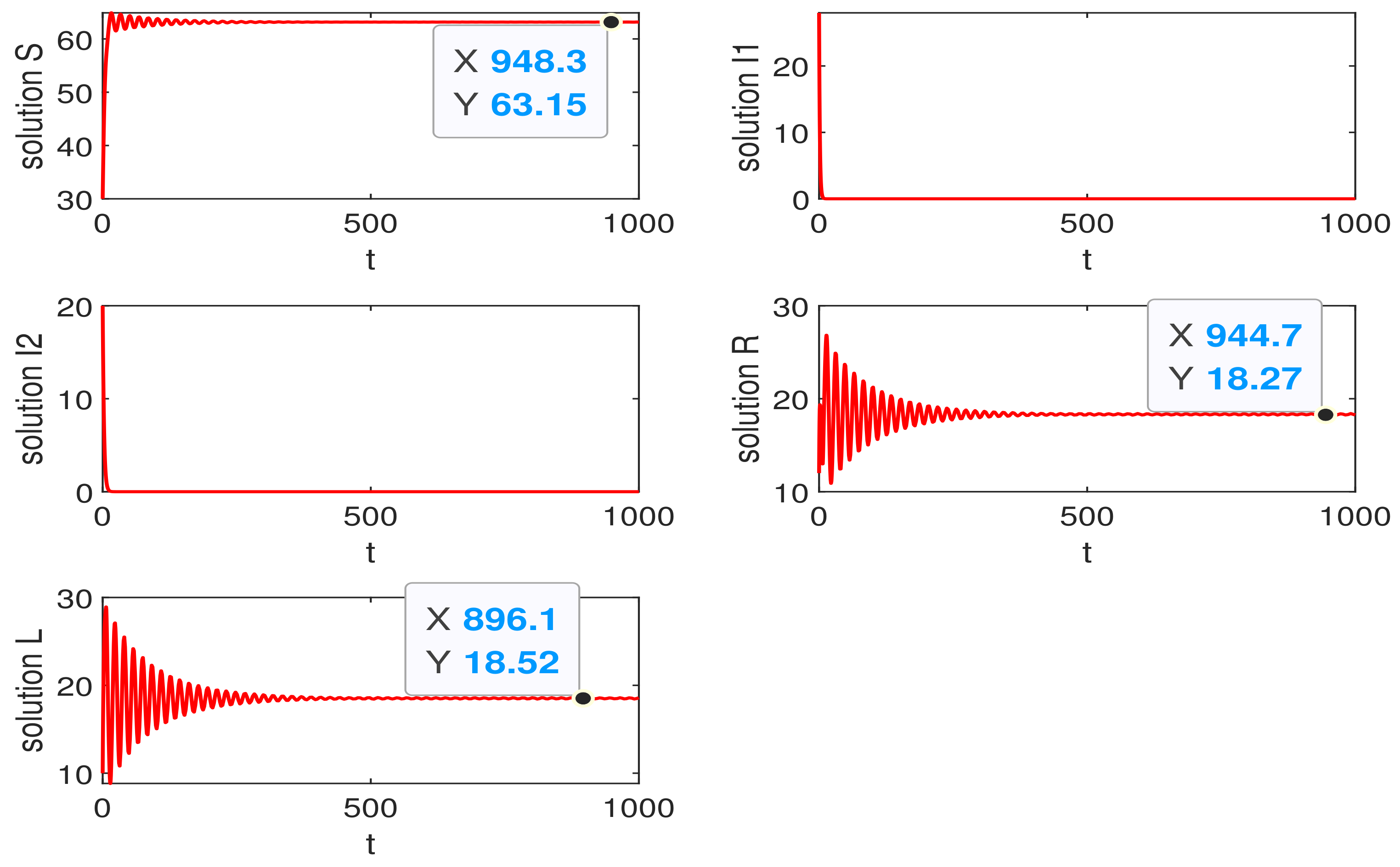
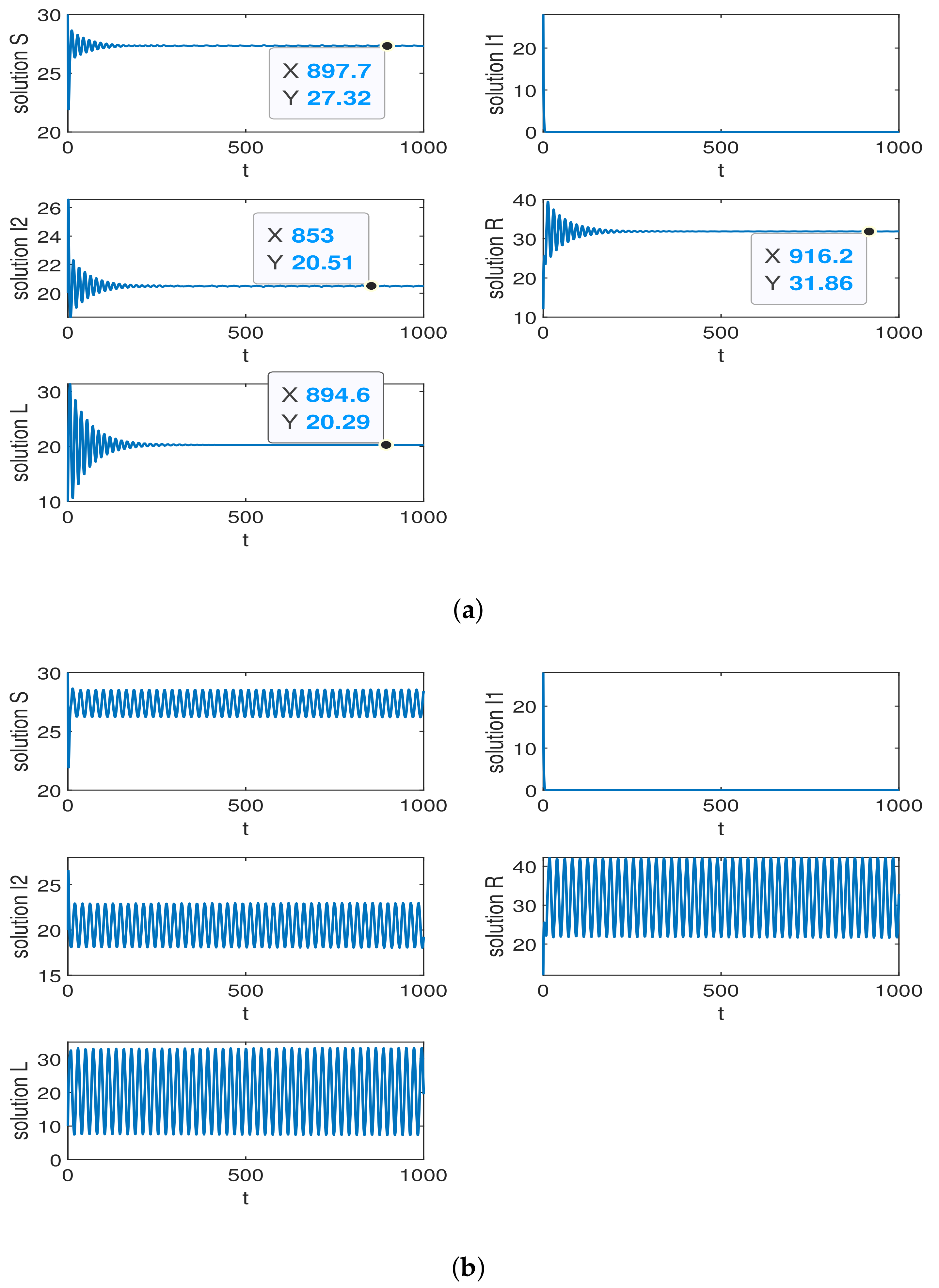
6.2. The Trend of the Quantity of State Nodes

In Section 2 and Section 3, the three solutions of the system (2) are calculated by analyzing and demonstrating. The following part will illustrate the theoretical results. The influence of different Hopf bifurcation points $\left(\tau \right)$ are illustrated. Through analyzing three conditions, including $E^0$, $\overline{E}$, and $E^{*}$, we can obtain the variation in the state nodes and the stable situation.

Firstly, the disease-free equilibrium and the basic reproductive numbers $R_1<1$ and $R_2<1$ need to be satisfied. Thus, the initial parameters are set as: $A=20$, ${\beta }_1=0.0029$, ${\beta }_2=0.003$, ${\gamma }_1=0.3$, ${\gamma }_2=0.2$, $c_1=0.15$, $c_2=0.22$, $\mu =0.46$, $d=0.2$, $ϵ=0.1$, and $\alpha =0.115$. Moreover, the initial value are S = 30, $I_1$ = 28, $I_2$ = 20, R = 12, and L = 10. The basic reproductive numbers can be obtained as $R_1=0.2021<1$ and $R_2=0.2726<1$, and the disease-free equilibrium is obtained as $E^0(63.1620,0,0,18.3199,18.5181)$. Obviously, the condition of Theorem 1 is satisfied. Then, by some complicated computations with Matlab software, we can obtain ${\omega }_0=0.2985$ and ${\tau }_{10}=8.1591$. As shown in Figure 2, there are different cases of the quantity of state nodes. It is shown that the system is locally asymptotically stable when $\tau =6.368<{\tau }_{10}$. From Figure 3a, it is shown that the system is unstable and goes into oscillation when $\tau =8.1593>{\tau }_{10}$. As shown in Figure 3b, the quantity of nodes has a particular variation like an elliptic curve. In a word, the quantity of $I_1$ and $I_2$ always tend to zero finally, whatever $\tau$ is.

To ensure $R_1<1$ and $R_2>1$, the initial parameters are set as $A=20$, ${\beta }_1=0.004$, ${\beta }_2=0.03$, ${\gamma }_1=0.2$, ${\gamma }_2=0.4$, $c_1=0.15$, $c_2=0.22$, $\mu =0.46$, $d=0.2$, $ϵ=0.4$, and $\alpha =0.2$, and the initial values are $S=30$, $I_1=28$, $I_2=20$, $R=12$, and $L=10$. Through computation, we can obtain $R_1=0.2241<R_2=2.0906$. It is obvious that this system has a fixed positive boundary equilibrium $\overline{E}=(27.3332,0,20.4987,31.8780,20.2900)$. It is easy to obtain ${\tau }_{20}=8.4822$. As shown in Figure 4a, the system is locally asymptotically stable if $\tau =5.891<{\tau }_{20}$. From Figure 4b, the system is unstable and goes into oscillation. In short, if the charging delay is $\tau <{\tau }_{20}$, the system will be stable eventually; if the charging delay $\tau$ is greater than the critical value ${\tau }_{20}$, the system will lose stability and goes into oscillation. The quantity of $I_1$ still tends to zero at the end of the time.

Lastly, considering the endemic equilibrium, it is necessary to ensure $R_1>1$ and $R_1>R_2$. The initial parameters are set as: $A=20$, ${\beta }_1=0.2$, ${\beta }_2=0.03$, ${\gamma }_1=0.15$, ${\gamma }_2=0.4$, $c_1=0.28$, $c_2=0.18$, $\mu =0.66$, $d=0.2$, $ϵ=0.2$, and $\alpha =0.45$. The basic reproductive numbers can be obtained as $R_1=11.4155>R_2=1.6026$. Thus, the endemic equilibrium is $E^{*}=(3.6501,39.0175,11.6384,25.5761,20.1179)$. The parameters are set to satisfy the Hopf condition, and the initial values of the nodes are set as $(S,I_1,I_2,R,L)=(20,35,10,20,15)$. We can obtain ${\omega }_{02}=0.4706$ and the critical value ${\tau }_{30}=4.9049$. As shown in Figure 5a, it is shown that the quantity of nodes of this system is from oscillation to stability when the charging delay $\tau =3.2049<{\tau }_{30}$. Thus, the system is locally asymptotically stable. From Figure 5b, if $\tau >{\tau }_{30}$, the system will be unstable and goes into oscillation, and this diagram is a particular condition that the system is a periodic oscillation.

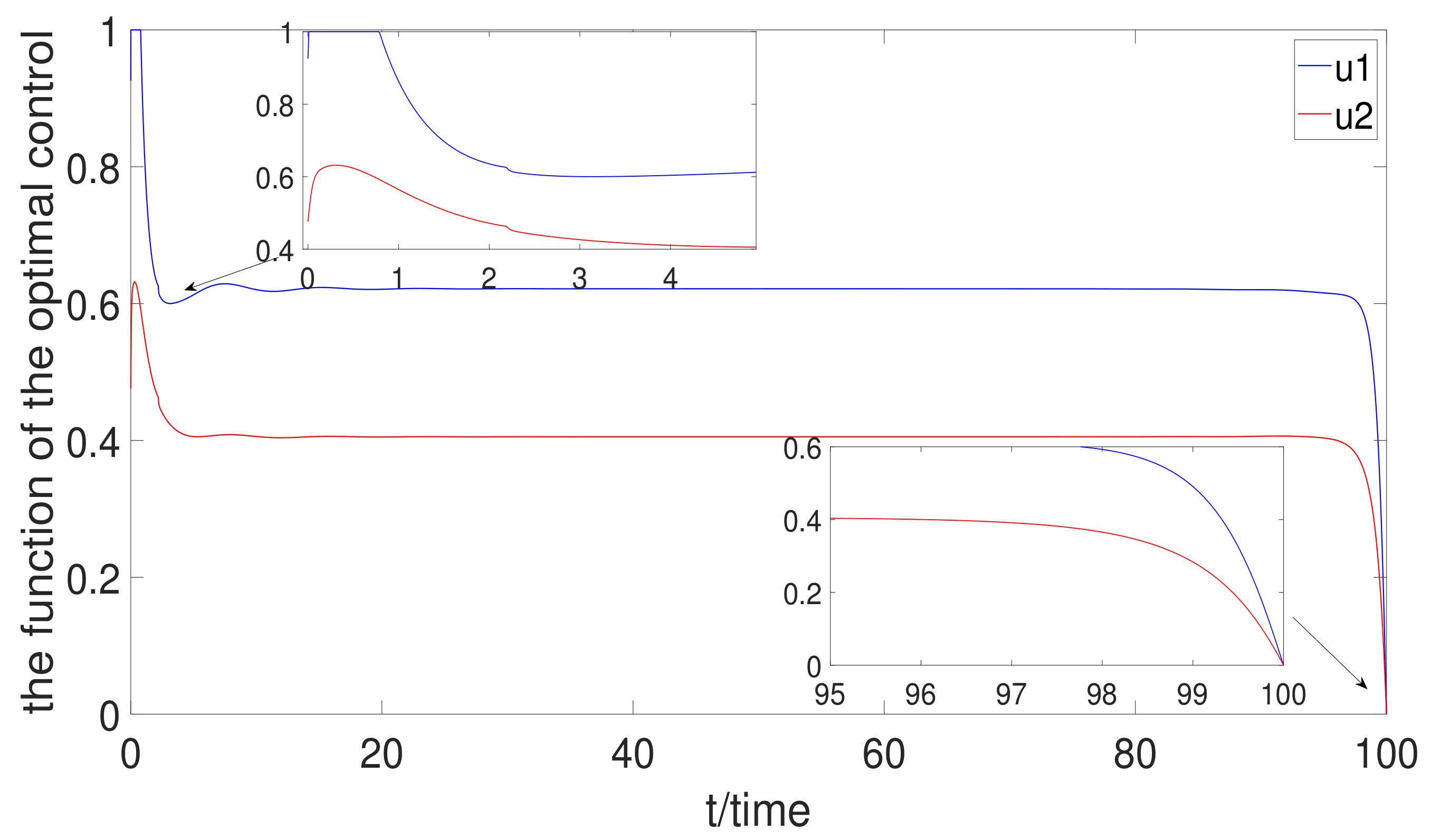
6.3. Optimal Control Strategy Analysis

In this part, the control factor is added to this system, and the optimal control method is proposed to consider the cost of treating the infected nodes. The theoretical analysis for the optimal control is demonstrated in Section 5. In this part, there are different methods of control, including maximum control, minimum control, average control, and optimal control [43].

The parameters are set as $A=20$, ${\beta }_1=0.389$, ${\beta }_2=0.1$, $c_1=0.15$, $c_2=0.22$, $\mu =0.56$, $ϵ=0.2$, $\alpha =0.115$, $d=0.2$, and $\tau =2.2$. The maximum control means full treatment; that is, the parameters’ values are set as ${\gamma }_1=1$ and ${\gamma }_2=1$. The minimum control means no treatment; that is, the parameters’ values are set as ${\gamma }_1=0$ and ${\gamma }_2=0$. The optimal control means ${\gamma }_1=u_1\left(t\right)$ and ${\gamma }_2=u_2\left(t\right)$; that is, $u_1\left(t\right)$ and $u_2\left(t\right)$ are the control curves of the patch input. Then, the average control is the average of the optimal control curve. When $m=30$ and $n=20$, the control curves are shown in Figure 6. Obviously, $u_1\left(t\right)$ is always greater than $u_2\left(t\right)$. As shown in Figure 7, we can obtain the curves of the cost for different methods. It is obvious that the cost of optimal control is the minimum. When $\tau =3.2$, the optimal control curve is shown in Figure 8. When $\tau =5.2$, the optimal control curve is shown in Figure 9. Thus, the larger the charging delay, the more oscillation appears in the optimal control curve.

When $\tau =2.2$, Figure 10 shows the ratio of different nodes for four control cases. For four cases, the proportion of S is the smallest and the proportion of R is the largest than the other state nodes of all the nodes. It is obvious that the ratios of $I_1$ and $I_2$ are lower for the full treatment than those for the no treatment. The ratio of $I_1$ decreases to $15.32\%$, and $I_2$ decreases to $3.11\%$. With the optimal control, the ratio of $I_1$ decreases to $18.67\%$ and $I_2$ decreases to $7.31\%$. Then, the average control can also control the ratios of $I_1$ and $I_2$.

As shown in Figure 11, the variation in nodes is shown. In addition to no treatment, the recovered nodes curve is the highest, which means that the number of recovered nodes is more than that of the other two control methods. The numbers $I_1$ and $I_2$ are less than that of no treatment. From Figure 11a, at the end of time, there is a noticeable wobble in the end of the optimal control curve.

In summary, according to the above analysis, the full treatment has the best effect to control the numbers of $I_1$ and $I_2$ when the control strategy of the system does not consider the cost. However, optimal control has the best effect to control the numbers of $I_1$ and $I_2$ when the control strategy of the system considers the cost.

7. Conclusions

In this paper, to investigate the malware propagation with charging delay and virus mutation in WRSNs, a new model is constructed and analyzed which improves the SIR model. The model involves a mutation which is caused by the infected variation. There is a charging delay in sensors. Unlike the SIR model, there are three equilibrium points including disease free equilibrium, boundary equilibrium, and endemic equilibrium. The analysis reveals the local stability of equilibrium points when the charging delay $\tau$ equals to zero. If $R_1$ < 1 and $R_2$ < 1, the malware does not affect the WRSNs and the malware will reduce to zero. In this charging delay model, the locally asymptotic stability is proven when $\tau$ is less than ${\tau }_0$. There are three different Hopf bifurcations.The system goes through a Hopf bifurcation, and the system goes into oscillation when $\tau$ is larger than ${\tau }_0$.

Meanwhile, the intent to study the SIIRL model of malware propagation in the WSN is used for controlling the spreading of mutation malware. We propose control strategies including full treatment control, average control, no treatment control, and optimal control. The cost relationships among the four control methods are $Optimal>Average>Full>No$. In addition, the malware proportion relationships among the four control methods are $Full>Optimal>Average>No$. Thus, considering the malware proportion and control cost, the best control method is optimal control. At the same time, the optimal control of the mutation model is also affected by the charging delay. The bigger the charging delay, the more oscillation appears in the optimal control curve. Finally, all of the theoretical analyses are proven by numerical simulation.

This paper discusses a mutation model with a charging delay. Although the dynamic propagation model is analyzed and the control strategy is proposed, there still exists an interesting work on how to establish rate of infection with actual situation. This work needs to be further studied in the future. However, with the development of networks, the heterogeneous network is one of our future research directions. Meanwhile, the stochastic model [50] and fractional order model [51] are also the trends in our future research.

References

1. Li, W.; Zhu, H. Research on Comprehensive Enterprise Network Security. In Proceedings of the 2021 IEEE 11th International Conference on Electronics Information and Emergency Communication (ICEIEC), Beijing, China, 18 20 June 2021; pp. 1–6. [Google Scholar]
2. Manshaei, M.H.; Zhu, Q.; Alpcan, T.; Bacşar, T.; Hubaux, J.P. Game theory meets network security and privacy. ACM Comput. Surv. (CSUR) 2013, 45, 1–39. [Google Scholar] [CrossRef]
3. Jing, Q.; Vasilakos, A.V.; Wan, J.; Lu, J.; Qiu, D. Security of the Internet of Things: Perspectives and challenges. Wirel. Netw. 2014, 20, 2481–2501. [Google Scholar] [CrossRef]
4. Sandra, S.H.; Natarajan, S.; Sakir, S. A survey of security in software defined networks. IEEE Commun. Surv. Tutorials 2015, 2015, 623–654. [Google Scholar]
5. Kulkarni, R.V.; Förster, A.; Venayagamoorthy, G.K. Computational intelligence in wireless sensor networks: A survey. IEEE Commun. Surv. Tutorials 2010, 13, 68–96. [Google Scholar] [CrossRef]
6. Farash, M.S.; Turkanović, M.; Kumari, S.; Hölbl, M. An efficient user authentication and key agreement scheme for heterogeneous wireless sensor network tailored for the Internet of Things environment. Ad Hoc Netw. 2016, 36, 152–176. [Google Scholar] [CrossRef]
7. Butun, I.; Morgera, S.D.; Sankar, R. A survey of intrusion detection systems in wireless sensor networks. IEEE Commun. Surv. Tutorials 2013, 16, 266–282. [Google Scholar] [CrossRef]
8. Ren, Q.C.; Liang, Q.L. Energy and quality aware query processing in wireless sensor database systems. Inf. Sci. 2007, 177, 2188–2205. [Google Scholar] [CrossRef]
9. Lenin, R.B.; Ramaswamy, S. Anosov flows with stable and unstable differentiable distributions. Ann. Oper. Res. 2015, 233, 237–261. [Google Scholar] [CrossRef]
10. Kephart, J.O.; White, S.R. Directed-graph epidemiological models of computer viruses. In Computation: The Micro and the Macro View; World Scientific: Singapore, 1992; pp. 71–102. [Google Scholar]
11. Kephart, J.O.; White, S.R. Measuring and modeling computer virus prevalence. In Proceedings of the 1993 IEEE Computer Society Symposium on Research in Security and Privacy, Oakland, CA, USA, 24–26 May 1993; pp. 2–15. [Google Scholar]
12. Liu, W.P.; Liu, C.; Yang, Z.; Liu, X.Y.; Zheng, Y.H.; Wei, Z.X. Modeling the propagation of mobile malware on complex networks. Commun. Nonlinear Sci. Numer. Simul. 2016, 37, 249–264. [Google Scholar] [CrossRef]
13. Zhu, L.H.; Zhou, X.; Li, Y.M. Global dynamics analysis and control of a rumor spreading model in online social networks. Phys. A Stat. Mech. Its Appl. 2019, 526, 120903. [Google Scholar] [CrossRef]
14. Li, J.X.; Ning, R.; Zhen, J. An SICR rumor spreading model in heterogeneous networks. Discret. Contin. Dyn.-Syst.-B 2020, 25, 1497. [Google Scholar] [CrossRef] [Green Version]
15. Choi, S.H.; Seo, H.; Yoo, M. A multi-stage SIR model for rumor spreading. Discret. Contin. Dyn. Syst.-B. 2020, 25, 2351. [Google Scholar] [CrossRef] [Green Version]
16. Huang, Y.A.; Tang, M.; Zou, Y.; Zhou, J. Hybrid phase transitions of spreading dynamics in multiplex networks. Chin. J. Phys. 2018, 56, 1166–1172. [Google Scholar] [CrossRef]
17. Khayam, S.A.; Radha, H. Using signal processing techniques to model worm propagation over wireless sensor networks. IEEE Signal Process. Mag. 2006, 23, 164–169. [Google Scholar] [CrossRef]
18. Feng, L.P.; Song, L.P.; Zhao, Q.S.; Wang, H.B. Modeling and stability analysis of worm propagation in wireless sensor network. Math. Probl. Eng. 2015, 2015, 129598. [Google Scholar] [CrossRef] [Green Version]
19. Singh, A.; Awasthi, A.K.; Singh, K.; Srivastava, P.K. Modeling and analysis of worm propagation in wireless sensor networks. Wirel. Pers. Commun. 2018, 98, 2535–2551. [Google Scholar] [CrossRef]
20. Ojha, R.P.; Srivastava, P.K.; Sanyal, G.; Gupta, N.S. Improved model for the stability analysis of wireless sensor network against malware attacks. Wireless Personal Commun. 2021, 116, 2525–2548. [Google Scholar] [CrossRef]
21. Muthukrishnan, S.; Muthukumar, S.; Chinnadurai, V. Optimal control of malware spreading model with tracing and patching in wireless sensor networks. Wirel. Pers. Commun. 2021, 117, 2061–2083. [Google Scholar] [CrossRef]
22. Ye, X.T.; Xie, S.S.; Shen, S.G. SIR1R2:Characterizing Malware Propagation in WSNs With Second Immunization. IEEE Access 2021, 9, 82083–82093. [Google Scholar] [CrossRef]
23. Gharaei, N.; Al-Otaibi, Y.D.; Rahim, S.; Alyamani, H.J.; Khani, N.A.K.K.; Malebary, S.J. Broker-Based Nodes Recharging Scheme for Surveillance Wireless Rechargeable Sensor Networks. IEEE Sens. J. 2021, 21, 9242–9249. [Google Scholar] [CrossRef]
24. Qin, C.; Sun, Y.H.; Zhang, Y.H.; Ai, M.T. A novel path planning of mobile charger in wireless rechargeable sensor networks. In Proceedings of the 2017 29th Chinese Control And Decision Conference (CCDC), Chongqing, China, 28–30 May 2017; pp. 2063–2067. [Google Scholar]
25. Lin, C.; Shang, Z.; Du, W.; Ren, J.K.; Wang, L.; Wu, G.W. CoDoC: A novel attack for wireless rechargeable sensor networks through denial of charge. In Proceedings of the IEEE INFOCOM 2019-IEEE Conference on Computer Communications, Paris, France, 29 April–2 May 2019; pp. 856–864. [Google Scholar]
26. Li, P.D.; Yang, L.X.; Yang, X.F.; Zhong, X.; Wen, J.H.; Xiong, Q.Y. Energy-efficient patching strategy for wireless sensor networks. Sensors 2019, 19, 262. [Google Scholar] [CrossRef] [PubMed] [Green Version]
27. Liu, G.Y.; Huang, Z.Y.; Wu, X.L.; Liang, Z.W.; Hong, F.H.; Su, X.K. Modelling and Analysis of the Epidemic Model under Pulse Charging in Wireless Rechargeable Sensor Networks. Entropy 2021, 23, 927. [Google Scholar] [CrossRef] [PubMed]
28. Liu, G.Y.; Su, X.K.; Hong, F.H.; Zhong, X.J.; Liang, Z.W.; Wu, X.L.; Huang, Z.Y. A Novel Epidemic Model Base on Pulse Charging in Wireless Rechargeable Sensor Networks. Entropy 2022, 24, 302. [Google Scholar] [CrossRef] [PubMed]
29. Keshri, N.; Mishra, B.K. Two time-delay dynamic model on the transmission of malicious signals in wireless sensor network. Chaos Solitons Fractals 2014, 56, 151–158. [Google Scholar] [CrossRef]
30. Zhang, Z.Z.; Zou, J.C.; Upadhyay, R.K.; ur Rahman, G. An epidemic model with multiple delays for the propagation of worms in wireless sensor networks. Results Phys. 2000, 19, 103424. [Google Scholar] [CrossRef]
31. Song, Y.L.; Wei, J.J. Local Hopf bifurcation and global periodic solutions in a delayed predator–prey system. J. Math. Anal. Appl. 2005, 301, 1–21. [Google Scholar] [CrossRef] [Green Version]
32. Xu, J.; Lu, Q.S. Hopf bifurcation of time-delay Lienard equation. Int. J. Bifurc. Chaos 1999, 9, 939–951. [Google Scholar] [CrossRef]
33. Wulf, V.; Ford, N.J. Numerical Hopf bifurcation for a class of delay differential equations. J. Comput. Appl. Math. 2000, 115, 601–616. [Google Scholar] [CrossRef] [Green Version]
34. Liu, G.Y.; Peng, B.H.; Zhong, X.J. A novel epidemic model for wireless rechargeable sensor network security. Sensors 2020, 21, 123. [Google Scholar] [CrossRef]
35. Nurtay, A.; Hennessy, M.G.; Sardanyés, J.; Alsedà, L.; Elena, S.F. Theoretical conditions for the coexistence of viral strains with differences in phenotypic traits: A bifurcation analysis. R. Soc. Open Sci. 2019, 6, 181179. [Google Scholar] [CrossRef] [Green Version]
36. Avllazagaj, E.; Zhu, Z.Y.; Bilge, L.; Balzarotti, D.; Dumitras, T. When Malware Changed Its Mind: An Empirical Study of Variable Program Behaviors in the Real World. In Proceedings of the 30th USENIX Security Symposium, online, 11–13 August 2021; pp. 3487–3504. [Google Scholar]
37. Li, D.M.; Li, C.C.; Xu, Y.J. The Stability of a Class of SEIR Epidemic Model with Virus Mutate. J. Harbin Univ. Sci. Technol. 2014, 19, 105–109. [Google Scholar]
38. Li, D.M.; Fu, Y.L.; Gao, T.Q.; Li, C.C. Stability analysis of a class of SIR epidemic model with delayed spontaneous variation of vrius. J. Harbin Univ. Sci. Technol. 2020, 25, 2. [Google Scholar]
39. Hao, R.J. Epidemic Spreading Model with Virus Variation and Its Stability; Nanjing University of Posts and Telecommunications: Nanjing, China, 2016. [Google Scholar]
40. Xu, D.G.; Xu, X.Y.; Su, Z.F. Novel SIVR epidemic spreading model with virus variation in complex networks. In Proceedings of the 27th Chinese Control and Decision Conference (2015 CCDC), Qingdao, China, 23–25 May 2015; pp. 5164–5169. [Google Scholar]
41. Cao, Y.L.; Wang, X.M.; He, Z.B. Optimal security strategy for malware propagation in mobile wireless sensor networks. Acta Electonica Sin. 2016, 44, 1851. [Google Scholar]
42. Zhang, L.; Liu, M.X.; Xie, B.L. Optimal control of an SIQRS epidemic model with three measures on networks. Nonlinear Dyn. 2021, 103, 2097–2107. [Google Scholar] [CrossRef]
43. Zhu, L.H.; Guan, G.; Li, Y.M. Nonlinear dynamical analysis and control strategies of a network-based SIS epidemic model with time delay. Appl. Math. Model. 2019, 70, 512–531. [Google Scholar] [CrossRef]
44. Chen, L.J.; Hattaf, K.; Sun, J. Optimal control of a delayed SLBS computer virus model. Phys. A Stat. Mech. Its Appl. 2015, 427, 244–250. [Google Scholar] [CrossRef]
45. Pei, Y.Z.; Chen, M.M.; Liang, X.Y.; Xia, Z.M.; Lv, Y.F.; Li, C.G. Optimal control problem in an epidemic disease SIS model with stages and delays. Int. J. Biomath. 2016, 9, 1650072. [Google Scholar] [CrossRef]
46. Li, L.L.; Sun, C.X.; Jia, J.W. Optimal control of a delayed SIRC epidemic model with saturated incidence rate. Optim. Control Appl. Methods 2019, 40, 367–374. [Google Scholar] [CrossRef]
47. Wan, C.; Li, T.; Zhang, W.; Dong, J. Dynamics of epidemic spreading model with drug-resistant variation on scale-free networks. Phys. A Stat. Mech. Its Appl. 2018, 493, 17–28. [Google Scholar] [CrossRef]
48. Liu, G.Y.; Peng, Z.M.; Liang, Z.W.; Li, J.Q.; Cheng, L.F. Dynamics Analysis of a Wireless Rechargeable Sensor Network for Virus Mutation Spreading. Entropy 2021, 23, 572. [Google Scholar] [CrossRef]
49. Liu, G.Y.; Chen, J.Y.; Liang, Z.W.; Peng, Z.M.; Li, J.Q. Dynamical Analysis and Optimal Control for a SEIR Model Based on Virus Mutation in WSNs. Mathematics 2021, 9, 929. [Google Scholar] [CrossRef]
50. Liu, Y.; Chu, D.H.; Zou, Y.X.; Su, H. Stabilization of stochastic complex networks with switching jump diffusions based on adaptive aperiodically intermittent control. Nonlinear Dyn. 2021, 104, 3737–3751. [Google Scholar] [CrossRef]
51. Achar, S.J.; Baishya, C.; Kaabar, K.A. Dynamics of the worm transmission in wireless sensor network in the framework of fractional derivatives. Math. Methods Appl. Sci. 2022, 45, 4278–4294. [Google Scholar] [CrossRef]
Figure 1. Relationship of the basic reproductive number and parameters. (a) The relationship among d, β 1 , and R 1 . (b) The relationship among d, β 2 , and R 2 .
Mathematics 10 02376 g001
Figure 2. The variation in the state nodes under τ = 6.368 < τ 10 .
Mathematics 10 02376 g002
Figure 3. τ = 8.1593 > τ 10 = 8.1591 . (a) The variation in the state nodes. (b) Left of Figure 3b is the relationship between S and R; right of Figure 3b is relationship between S and L.
Mathematics 10 02376 g003
Figure 4. The variation diagram of state nodes. (a) The variation in the state nodes when τ = 5.891 < τ 20 = 8.4822 . (b) The variation in the state nodes when τ = 8.4922 > τ 20 .
Mathematics 10 02376 g004
Figure 5. The variation diagram of state nodes. (a) The variation in the state nodes when τ = 3.2049 < τ 30 = 4.9049 . (b) The variation in the state nodes when τ = 4.9050 > τ 30 .
Mathematics 10 02376 g005
Figure 6. The optimal control curves when τ = 2.2.
Mathematics 10 02376 g006
Figure 7. The cost curves.
Mathematics 10 02376 g007
Figure 8. The optimal control curves when τ = 3.2.
Mathematics 10 02376 g008
Figure 9. The optimal control curves when τ = 5.2.
Mathematics 10 02376 g009
Figure 10. The diagram of proportion of nodes.
Mathematics 10 02376 g010
Figure 11. Variation in node numbers: (a) Optimal control; (b) No treatment control; (c) Average control; (d) Full treatment control.
Mathematics 10 02376 g011