Research on Maximum Likelihood b Value and Confidence Limits Estimation in Doubly Truncated Apparent Frequency–Amplitude Distribution in Rock Acoustic Emission Tests

Abstract

The b value deduced from the Gutenberg–Richter law is an important parameter for sequence and precursory analyses, both in laboratory acoustic emission tests and seismology. As the b value is a statistical value, the maximum likelihood estimation is mostly used to estimate the b value. However, traditional singly truncated maximum likelihood estimation in seismology only considers the minimum magnitude, while the acquisition device in rock acoustic emission tests will set the threshold value and maximum value of the amplitude; therefore, maximum likelihood estimation will estimate the b value in a doubly truncated size distribution, and its confidence limits need to be discussed. Here, in this study, we derive the calculation equations of the b value and the corresponding confidence limits for the maximum likelihood estimation with a narrow amplitude span in a doubly truncated frequency–amplitude distribution. The maximum likelihood b values estimated by the scheme of a singly and doubly truncated frequency–amplitude distribution are compared through acoustic emission data with the known underlying distribution. The results show that the maximum likelihood b value and confidence limits estimation scheme derived for rock acoustic emission tests with a narrow amplitude span is more reasonable. Then, the derived estimation scheme is applied to the rock dilation rupturing test; the results confirm its applicability.

1. Introduction

In seismology, the Gutenberg–Richter (G-R) law [1] has long been one of the major important research areas in the problems concerning the statistical analyses of earthquakes. The G-R law is expressed on a logarithmic scale, which is equivalent to the source energy E and seismic moment M₀ obeying a power–law relationship. Many researchers in the field of seismology have used the G-R law to describe the size distribution and analyze probabilistic seismic hazards. The G-R law is given by:

$${\log }_{10}(N)=a-bM$$

(1)

where M is the magnitude, N is the number of earthquakes that occur in the specific space–time window with a magnitude greater than or equal to M; a and b are constants, where b is also referred to as the b value, which is a significant scale parameter for operational earthquake forecasting and material heterogeneity and differential stress analysis [2].

In the calculation of the b value through Equation (1), the selection of the estimation method greatly influences the b-value estimation result. The corresponding confidence limits are also important, and can evaluate the correctness and reliability of the estimated b value [3]. Since the G-R law was proposed, the least square regression (LSR) has been used by many scholars to estimate the b value due to its simplicity. LSR that obeys the Gaussian distribution error is suitable for equal weight data points fitting. However, both cumulative and incremental frequency–magnitude distributions are obtained by binning the magnitude, which is in contradiction with the Gaussian error assumption of LSR. As a result, too much weight is given to the relatively few large shocks and too little to the many small events [4]. Furthermore, the confidence limits determined by the LSR are unrealistically small. Consequently, the maximum likelihood estimation (MLE) is introduced in statistical seismology, which assigns the same weight to all earthquakes, so many studies suggest using the MLE instead of LSR to calculate the b value [5,6,7]. Additionally, since the selection of amplitude limits of the ‘linear range’ of the frequency–amplitude distribution and estimation method has a great influence on the calculation of the b value, considering the mean and standard deviation of the AE amplitude sample, Shiotani proposed the parameter of the Ib value (improved b value), which is also widely used to evaluate and monitor the fracture behavior of materials. Many studies have shown that the Ib value and the b value are different in size, but the change trend is the same [8,9,10].

Originally, the b value and corresponding confidence limits estimated by MLE were usually carried out in a singly truncated frequency–magnitude distribution, which only considers the minimum magnitude. However, many scholars have found that maximum magnitude does exist for a considered seismic region [11,12,13,14,15,16,17]; so the b value and corresponding confidence limits estimation should be performed in a doubly truncated frequency–magnitude distribution [18].

As the heterogeneous state of the earth and the inaccessibility of the fault zone for direct measurement limit earthquake mechanism research [16], an increasing number of scholars hope to analyze the mechanism and precursor characteristics of earthquakes through the analogy of laboratory rock acoustic emission (AE) tests [19,20,21,22,23,24]. At the same time, the AE technique has often been used to study the destruction properties by recording the radiated elastic wave in the process of crack initiation, propagation and coalescence during rock deformation [25,26,27,28,29]. Meanwhile, in the study of AE characteristics in rock deformation tests, the analysis of the b value is also a focus [30,31,32,33]. The amplitudes of AE signals are always used for the b-value estimation, and amplitudes are usually divided by 20 to produce a b value comparable to that reported in the seismic literature [34,35,36]. However, the amplitude range received by sensors in laboratory rock AE tests is set between the threshold and maximum output value to reduce the interference of background noise and consider the maximum energy released by rock failure, so the lower and upper limits of the amplitude are determined [37]. Therefore, the b value and corresponding confidence limits in rock AE tests will be estimated in such a doubly truncated frequency–amplitude distribution (DTFAD) when MLE is employed.

In addition, the amplitudes used for the b-value estimation in laboratory rock AE tests are the apparent amplitudes measured on the sample boundary, which are attenuated from the sources, and the corresponding apparent frequency–amplitude distribution is not the size distribution of the sources, so the attenuation may modify the b value. This was discussed in detail in our previous research [38], and we theoretically proved that the b value is unchanged within an amplitude interval specified by the minimum and maximum amount of attenuation; further we proposed a new method called FGS (Fisher optimal split and Global Search algorithm) to determine this amplitude interval and estimate the b value. This means that a secondary truncation is performed in the original DTFAD, which leads to a narrower amplitude span (span between the minimum and maximum amplitude truncated by FGS for the b-value estimation) and smaller data volume in the frequency–amplitude distribution segment determined by FGS. Therefore, considering that the frequency–amplitude distribution of rock AE tests is a DTFAD, and the influence of attenuation effect on the b value, the generally used b value and confidence limits estimation method of MLE in a singly truncated distribution is not suitable for the b-value analysis. Consequently, the use of MLE to estimate the b value and determine the corresponding confidence limits with such a narrow amplitude span in rock AE tests needs to be further discussed.

In this study, we firstly use MLE to derive the equations for the b-value estimation and confidence limits determination with a narrow amplitude span for rock AE tests. In order to verify the performance of the derived MLE confidence limits, we generate synthetic AE data with the source amplitude subject to exponential distribution according to the simulation scheme in our previous study [30], and compare the performance of the newly derived MLE b value and confidence limits estimation scheme with Aki’s [39]. Then, we further investigate the applicability of the newly derived MLE b value and confidence limits estimation scheme in a specifically designed rock deformation test. This paper can improve the performance of MLE for the b-value estimation in the rock AE test, and in turn, enhance the reliability of the precursory analysis of rock failure through the AE b value.

2. Derivation of MLE b Value and Confidence Limits Estimation Scheme in DTFAD for Rock AE Tests

To avoid the potential error in calculating the b value by the LSR with equal weights, Aki [39] proposed a different method, in which the b value is given by

$${\log }_{10}e/(\overline{M}-M_0)$$

(2)

where $\overline{M}$ is the average magnitude in a given sample, $M_0$ is the minimum magnitude considering data completeness (considering the round-off of the magnitude and $M_0$ is usually replaced by $M_c=M_0-\Delta M/2$, where $\Delta M$ is the magnitude bins). Then, Aki deals with the earthquake catalogue with magnitude greater than $M_0$, and assumes that the probability density function $f(M,b^{\prime })$ is expressed by

$$f(M,b^{\prime })=b^{\prime }{e}^{-b^{\prime }(M-M_0)},M_0\le M$$

(3)

where $b^{\prime }=b/{\log }_{10}e$. Through maximum likelihood derivation and central limit theorem, the final b value is the same as Utsu’s [40], and confidence limits of the b value in a singly truncated distribution are given by

$$\frac{(1-d_{\epsilon }/\sqrt{n})}{{\displaystyle \sum _1^n{M}_i/n-M_0}}\le b^{\prime }\le \frac{(1+d_{\epsilon }/\sqrt{n})}{{\displaystyle \sum _1^n{M}_i/n-M_0}}$$

(4)

where n is the number of earthquakes in a given sample, M_i is the magnitude of i-th earthquake in the sample and $d_{\epsilon }$ = 1.96 when the confidence level is 95%.

In rock AE tests, amplitudes of AE signals are used for the b-value estimation, and threshold voltage value and the maximum voltage value of received signals are usually set on the acquisition equipment, so the frequency–amplitude distribution of AE signals will be in a doubly truncated range; obviously, maximum likelihood confidence limits in a singly truncated distribution are not suitable. Additionally, the segment for the b-value estimation in DTFAD will be very small as the FGS method is adopted, and the data volume will be correspondingly reduced. Therefore, in this section, we discuss the confidence limits of the b value by MLE in DTFAD under a narrow amplitude span and small data volume in rock AE tests.

As we know, when the source amplitude X > 0, the density function of exponential distribution is

$$f\left(x\right)=\left\{\begin{array}{l}\alpha e^{-\beta x} x>0\\ 0 x\le 0\end{array}\right.$$

(5)

where $\alpha$ and $\beta$ are constants. It can be obtained that the density function in a truncated exponential distribution at the range of $x\in [a_1,a_2]$ is as follows:

$$f\left(x\right)=\left\{\begin{array}{l}\alpha e^{-\beta x} a_1\le x\le a_2\\ 0 \mathrm{otherwise}\end{array}\right.$$

(6)

The distribution function can be approximated as

$$F_X\left(x\right)={\displaystyle {\int }_{-\infty }^{x}f\left(x\right)dx}=\left\{\begin{array}{l}1 x>a_2\\ {\displaystyle {\int }_0^x\alpha e^{-\beta x}dx} a_1\le x\le a_2\\ 0 \mathrm{otherwise}\end{array}\right.$$

(7)

We can solve that

$$\alpha =\beta \frac{e^{\beta a_1}}{1-e^{\beta (a_1-a_2)}}$$

(8)

Thus, the expectation $\mu$ and variance ${\sigma }^2$ are

$$\mu =E\left(X\right)=\frac{a_1+\frac{1}{\beta }}{1-e^{\beta (a_1-a_2)}}+\frac{a_2+\frac{1}{\beta }}{1-e^{\beta (a_2-a_1)}}=\frac{1}{\beta }+\frac{a_1-a_2{e}^{\beta \left(a_1-a_2\right)}}{1-e^{\beta \left(a_1-a_2\right)}}$$

(9)

$${\sigma }^2=D\left(X\right)=\left[\frac{{a_1}^2+\frac{2}{\beta } a_1+\frac{2}{{\beta }^2}}{1-e^{\beta (a_1-a_2)}}+\frac{{a_2}^2+\frac{2}{\beta } a_2+\frac{2}{{\beta }^2}}{1-e^{\beta (a_2-a_1)}}\right]-{\left[\frac{a_1+\frac{1}{\beta }}{1-e^{\beta (a_1-a_2)}}+\frac{a_2+\frac{1}{\beta }}{1-e^{\beta (a_2-a_1)}}\right]}^2$$

(10)

According to the doubly truncated probability density function Equation (6) of AE events, the joint probability density function of the amplitude samples can be obtained as

$$f(x_1,x_2,\cdots ,x_N\left|\beta \right.)={\displaystyle \prod _{i=1}^N\alpha e^{-\beta x_i}}$$

(11)

Combining Equation (8), we can construct the likelihood function:

$$\begin{array}{l}L=\ln \left[f(x_1,x_2,\cdots ,x_N\left|\beta \right.)\right]\\ =N\ln \alpha -\beta {\displaystyle \sum _{i=1}^N{x}_i}\\ =N\ln \beta +N\beta a_1-N\ln (1-e^{\beta (a_1-a_2)})-\beta {\displaystyle \sum _{i=1}^N{x}_i}\end{array}$$

(12)

Here, when we only consider one parameter $\beta$, let the partial derivative of the likelihood function L with respect to $\beta$ be 0:

$$\frac{\partial L}{\partial \beta }=\frac{N}{\beta }+N{a}_1-\frac{-N(a_1-a_2)e^{\beta (a_1-a_2)}}{1-e^{\beta (a_1-a_2)}}-{\displaystyle \sum _{i=1}^N{x}_i}=0$$

(13)

So, we can get that

$$\frac{1}{\widehat{\beta }}+\frac{a_1-a_2{e}^{\widehat{\beta }(a_1-a_2)}}{1-e^{\widehat{\beta }(a_1-a_2)}}=\overline{x}$$

(14)

It can be seen from Equations (9) and (14) that the b value obtained by MLE is the same as the moment estimation, which shows the correctness of the obtained b value in DTFAD. If $a_2$ approaches infinity or $a_2$ is much larger than $a_1$ ($a_2-a_1>2~3$), Equation (14) can be simplified to Equation (2) [41]. However, $a_1$ and $a_2$ do not satisfy this condition, as the FGS method is used to perform a secondary truncation in DTFAD, and the b value by MLE must be calculated from Equation (14) instead of Equation (2).

Therefore, the confidence limits in DTFAD of the parameter $\beta$ are as follows:

$$\begin{array}{l}\mu =h(\beta )=\frac{1}{\beta }+\frac{a_1-a_2{e}^{\beta (a_1-a_2)}}{1-e^{\beta (a_1-a_2)}}\\ \frac{\partial }{\partial \mu }\ln (L(x_1,x_2,\cdots ,\alpha ,\beta ))=(\mu -\overline{x})\times \frac{N}{h^{\prime }(\beta )}=0\end{array}$$

(15)

From $\widehat{\beta }=\overline{X}$ and Cramer–Rao inequality, it can be judged that the estimation is the optimal estimation. $\widehat{\mu }=h(\widehat{\beta })=\overline{X}=E(\widehat{\mu })=E(\overline{X})$, so, inequalities of both sides are equal; that is:

$$D(\widehat{\mu })=\frac{1}{-E\left[\frac{{\partial }^2\ln p(x\left|\mu \right.)}{\partial {\mu }^2}\right]}=\frac{1}{-E{{\left[(\mu -\overline{x})\times \frac{N}{h^{\prime }(\beta )}\right]}^{\prime }}_{\mu }}=-\frac{h^{\prime }(\beta )}{N}$$

(16)

Since $h(\beta )$ will decrease monotonically with $\beta$, when ${\beta }_1<{\beta }_2$, let $|\mu -\widehat{\mu }|<\epsilon$, $\widehat{\mu }+\epsilon =\frac{1}{\widehat{{\beta }_1}}+\frac{a_1-a_2{e}^{\beta (a_1-a_2)}}{1-e^{\beta (a_1-a_2)}}$, $\widehat{\mu }-\epsilon =\frac{1}{\widehat{{\beta }_2}}+\frac{a_1-a_2{e}^{\beta (a_1-a_2)}}{1-e^{\beta (a_1-a_2)}}$, and $\widehat{\mu }=\overline{X}=\frac{1}{\widehat{\beta }}+\frac{a_1-a_2{e}^{\beta (a_1-a_2)}}{1-e^{\beta (a_1-a_2)}}$, according to Chebyshev’s inequality:

$$p\{\widehat{{\beta }_1}<\beta <\widehat{{\beta }_2}\}=p\left\{\right|\mu -\widehat{\mu }|<\epsilon \}>1-\frac{D(\widehat{\mu })}{{\epsilon }^2}=1+\frac{h^{\prime }(\beta )}{N{\epsilon }^2}\approx 1+\frac{h^{\prime }(\widehat{\beta })}{N{\epsilon }^2}$$

(17)

From $b=\beta \times 20/\ln (10)$, the maximum likelihood confidence limits of the b value with a narrow amplitude span in DTFAD can be obtained using Equation (17).

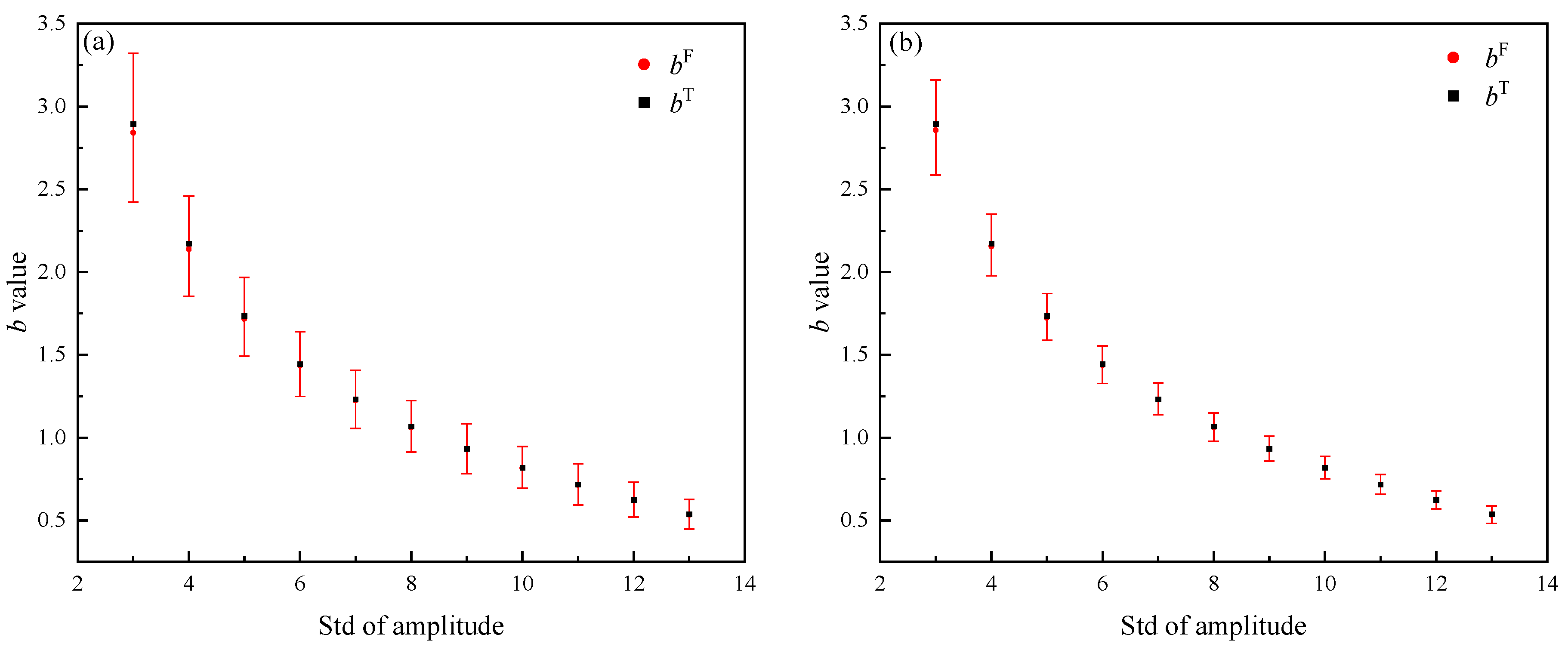
3. Performance Verification of the Derived MLE b Value and Confidence Limits Estimation Scheme in DTFAD Based on Synthetic Data

Because the source amplitude data in laboratory tests cannot be processed to obtain the known underlying distribution and the real b value, here, we randomly generate AE amplitude data with known underlying distribution by computer to facilitate the performance verification of the derived MLE b value and confidence limits estimation scheme in DTFAD. Since the amplitudes used for the b-value estimation in laboratory rock AE tests are the apparent amplitude measured on the sample boundary by an acoustic sensor which is attenuated from the source, we generate two columns of data of source amplitudes and attenuation amount with the same length which are all in decibels with a round-off interval of 1 dB, respectively, and the apparent amplitude outputted by the sensor can be obtained by randomly subtracting the attenuation amount from the source amplitude. This synthetic data generation procedure is based on the concept proposed by Liu et al. [38] for the research of the attenuation effect on the size distribution and the b value, and the specific procedure of synthetic AE data generation is described in our previous research by Chen et al. [30]. As the range of the b value in general research is 0–3 [42], the source amplitudes with the data volumes of 300, 500, 800, 1000, 2000, 3000, 5000, 8000, 10,000, 50,000 and 100,000 at three theoretical b value (b₁^T = 2.1715, b₂^T = 1.0666 and b₃^T = 0.6245, b^T represents the theoretical b value of generated amplitude data with known underlying distribution) are generated in the source amplitude range of 50~109 dB, and the attenuation amount is generated in the range of 3~20 dB.

The frequency–amplitude distribution of apparent amplitude data is a DTFAD, then we adopt the FGS method to search the left and right endpoint and determine the log-linear segment that still obeys the G-R law after attenuation for the b-value estimation. The b values and confidence limits of three theoretical b values under different data volumes are shown in

Table 1. b values and corresponding confidence limits estimated by MLE.

Data Volume	bT	bA	bF	Confidence Limits of bF		Segment Determined by FGS
				Lower	Upper	Left Endpoint	Right Endpoint	Span/20
300	2.1715	3.2272	2.0804	0.7956	4.0562	40.71	48.55	0.3920
	1.0666	2.4161	1.0753	0.2272	2.3090	41.96	53.46	0.5750
	0.6245	1.7274	0.5716	0.1478	1.4862	43.92	62.64	0.9360
500	2.1715	3.2211	2.1098	1.0917	3.5840	40.50	48.24	0.3870
	1.0666	2.1184	1.0090	0.4725	1.7834	41.61	53.22	0.5805
	0.6245	1.9165	0.6119	0.2102	1.1016	43.68	58.36	0.7340
800	2.1715	3.0030	2.1350	1.3169	3.2732	40.42	48.83	0.4205
	1.0666	2.0981	1.0634	0.5701	1.6672	42.15	54.49	0.6170
	0.6245	1.6907	0.5981	0.2518	1.0192	43.03	58.34	0.7655
1000	2.1715	2.9978	2.1307	1.3936	3.0845	40.37	48.75	0.4190
	1.0666	2.0112	1.0649	0.5634	1.6356	42.05	54.70	0.6325
	0.6245	1.4890	0.6068	0.3329	0.9525	43.74	61.26	0.8760
2000	2.1715	2.7451	2.1751	1.6421	2.4591	40.22	50.31	0.5045
	1.0666	1.8940	1.0618	0.7085	1.4579	41.73	54.83	0.6550
	0.6245	1.1968	0.6191	0.4270	0.8486	44.11	66.35	1.1120
3000	2.1715	2.6223	2.1502	1.7768	2.5957	40.21	51.60	0.5695
	1.0666	1.6856	1.0676	0.8410	1.3162	40.96	57.22	0.8130
	0.6245	1.0594	0.6190	0.4856	0.7686	42.56	67.91	1.2675
5000	2.1715	2.4491	2.1387	1.8641	2.4501	40.16	53.52	0.6680
	1.0666	1.4626	1.0627	0.9261	1.2111	40.68	60.44	0.9880
	0.6245	0.9476	0.6224	0.5268	0.7226	41.94	71.78	1.4920
8000	2.1715	2.3873	2.1558	1.9541	2.3842	40.10	55.16	0.7530
	1.0666	1.2874	1.0645	0.9721	1.1652	40.28	64.87	1.2295
	0.6245	0.8366	0.6209	0.5616	0.6840	41.67	75.96	1.7145
10,000	2.1715	2.3371	2.1548	1.9770	2.3495	40.02	55.52	0.7750
	1.0666	1.2592	1.0612	0.9782	1.1495	40.26	65.82	1.2780
	0.6245	0.8086	0.6226	0.5694	0.6784	41.27	77.59	1.8160
50,000	2.1715	2.1990	2.1558	2.0857	2.2296	40.14	62.15	1.1005
	1.0666	1.1207	1.0653	1.0356	1.0961	40.04	77.32	1.8640
	0.6245	0.7092	0.6245	0.6058	0.6436	40.14	86.99	2.3425
100,000	2.1715	2.1709	2.1608	2.1146	2.2087	40.00	65.19	1.2595
	1.0666	1.1011	1.0655	1.0454	1.0861	40.00	81.30	2.0650
	0.6245	0.6962	0.6242	0.6115	0.6372	40.04	89.26	2.4610

, b^T is the theoretical b value of generated source amplitude data, b^A is the b value calculated by MLE of Aki’s equation (Equation (2) in this paper). b^F is the b value calculated by MLE of Equation (14); the confidence limits are calculated according to Equation (17) with a 95% confidence level. It can be seen that as the data volume increases, the deviation of the calculated b value from b^T gradually decreases, but the deviation between b^A and b^T is much larger than that between b^F and b^T when the data volume is small. The log-linear segment span determined by FGS increases with the increase in data volume; the segment span/20 will approach two only when the data volume exceeds 10,000 and b^T is small. Therefore, when the data volume and segment span for the b-value estimation are small, Equation (14) can be used to obtain a more accurate b value. Meanwhile, the data volume used for the b-value estimation is greatly reduced because of the truncation by FGS in DTFAD to search for the log-linear segment that still obeys the G-R law, so the width of confidence limits of b^F is large when the data volume is small and gradually narrows with the increase in data volume.

Furthermore, in addition to data volume, the accurate estimation of the b value will also be affected by the value of b^T. Figure 1 shows the b^F estimated by MLE and corresponding confidence limits with various b^T; obviously, the deviation between b^F and b^T is getting smaller, and the corresponding confidence limits are getting narrower with the decrease in b^T. The reason for this can be attributed to data incompleteness: the computer will generate a greater data volume with a smaller amplitude and lesser data volume with a larger amplitude when a larger b^T is set, which leads to poor data completeness and deviation from the G-R law of frequency–amplitude distribution at the right end [30]. Correspondingly, when b^T is set to be smaller, a greater data volume of amplitude will be generated, and better data completeness at the right end of the frequency–amplitude distribution will be obtained. Another phenomenon worth noting is that the width of the confidence limits will also become narrower as the b^T decreases. The confidence limits are an important reference for the stability of the estimated value; generally, the smaller the confidence limits, the more stable the statistical value. So here again, from the perspective of the confidence limits, the preset b^T will affect the calculation stability of the b value.

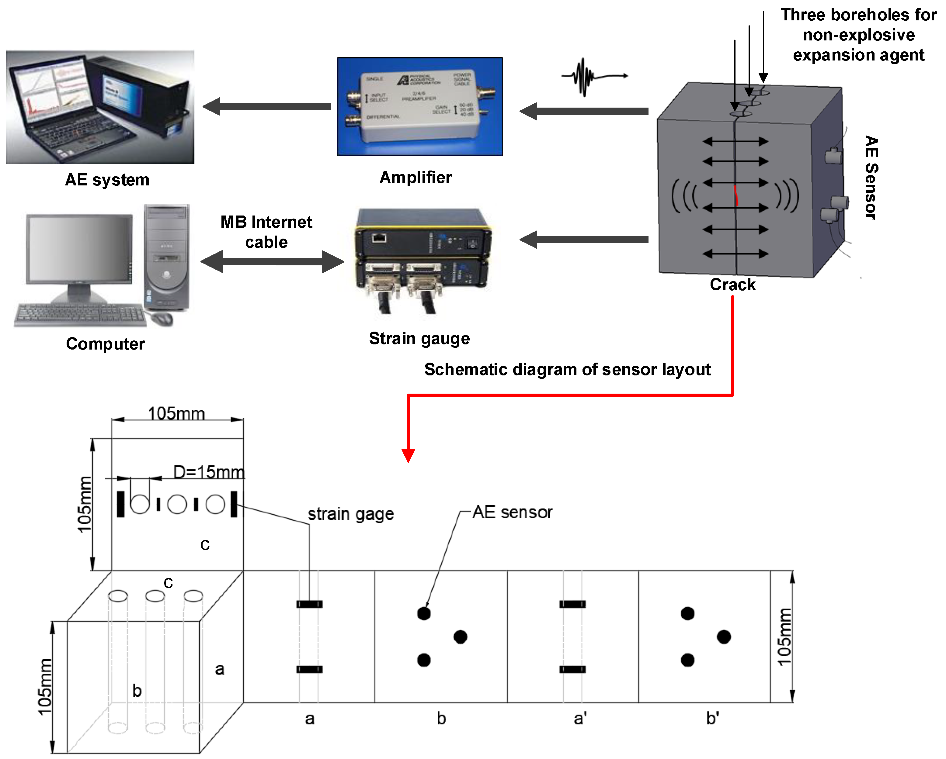
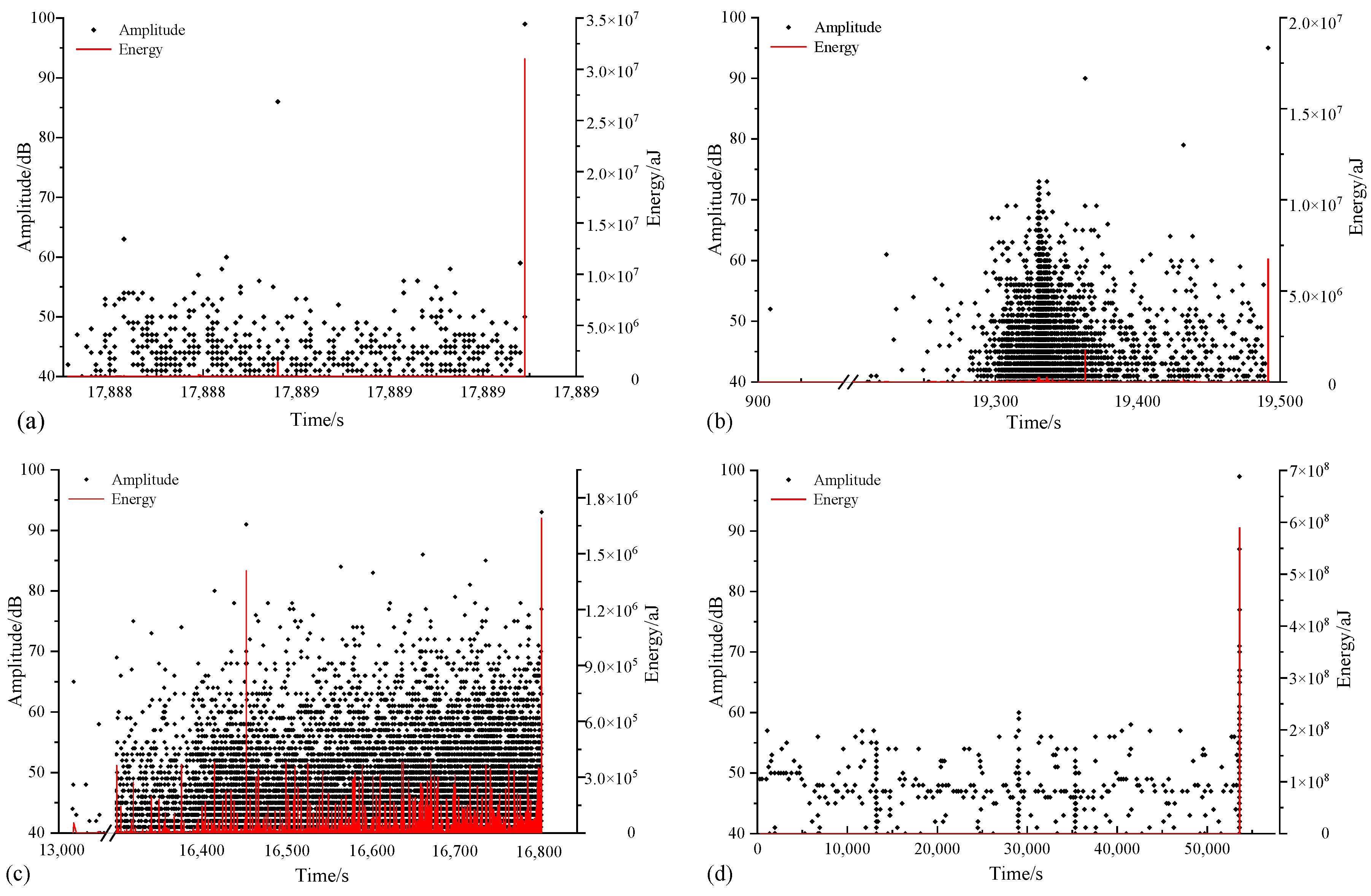
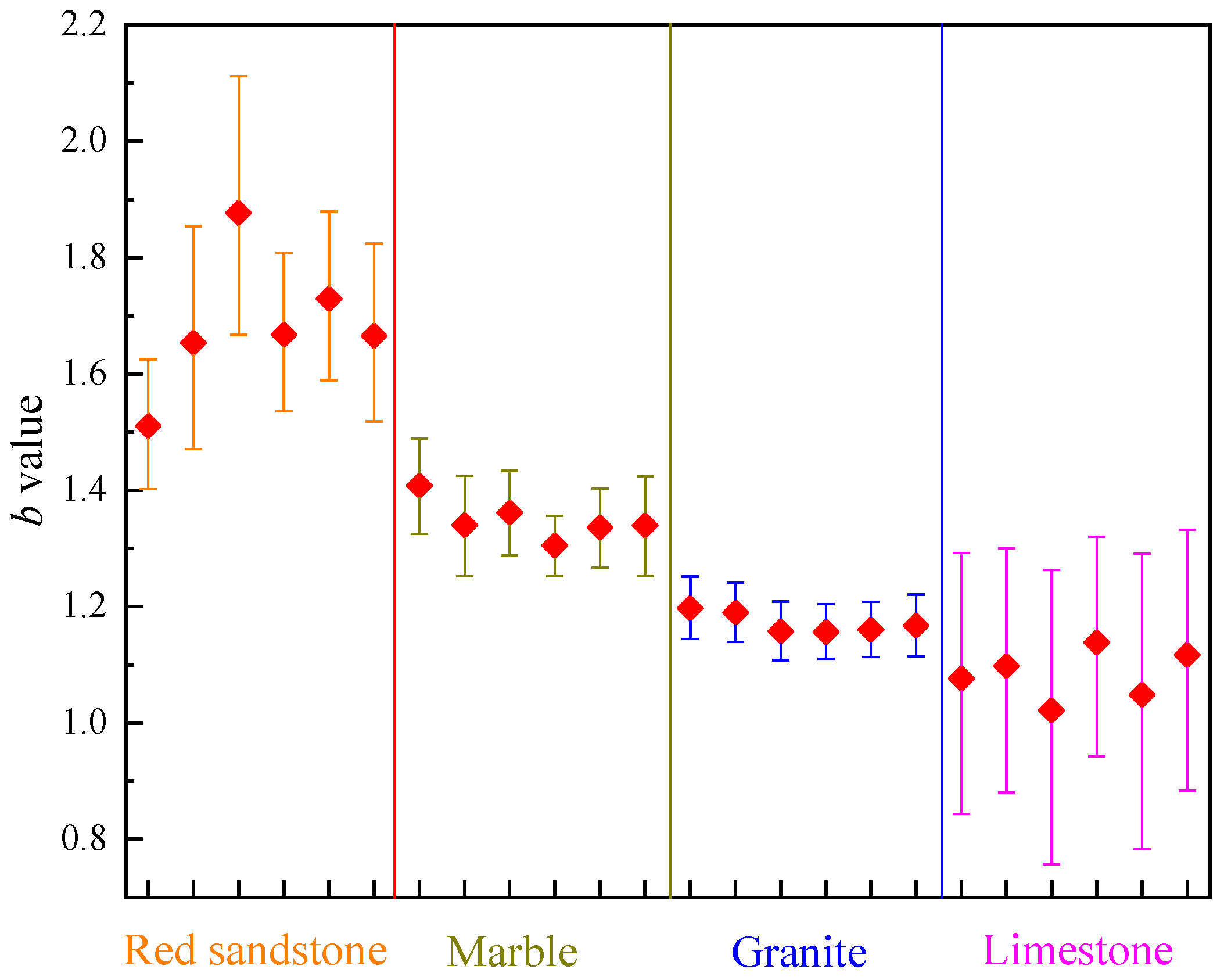
4. Applicability of the MLE b Value and Confidence Limits Estimation Scheme in Specifically Designed Rock Deformation Test

The b value reflects the characteristic relationship of the AE frequency–amplitude distribution during the deformation of the rock; that is, the number of small-scale failure events is much larger than the number of large-scale failures. So, the b value will be dominated by the number of small events, and small events are mainly generated in areas with large rock anisotropy [43,44,45]; different types of rocks should have different size distribution characteristics. Therefore, based on the correlation between the b value and the internal structure of different types of rocks, we can verify the correctness of the derived MLE b value and confidence limits estimation scheme in DTFAD. Here, we design a static dilation rock rupturing AE test by injecting a non-explosive cracking agent into three predrilled boreholes to form a specific fracture surface in a cubic rock specimen; this experimental design is to ensure that the sensor-collected AE signals are all generated via expansion rupturing in rock specimens, and do not rely on the source location to identify valid rupturing data [32].

Red sandstone, marble, granite and limestone are selected to carry out the non-explosive fracturing agent expansion rock AE test; the applicability of the b value and confidence limits in DTFAD calculated by MLE is further discussed. The specific experimental process, rock mass size and AE sensors distribution are shown in Figure 2.

Consequently, Figure 3 shows the microstructure map of the rock, Figure 4 shows the distribution of AE amplitude and energy with time in the process of expansion and failure of four kinds of rocks, and Figure 5 shows the MLE b values and confidence limits in DTFAD of red sandstone, marble, granite and limestone, and the specific calculation results are listed in

Table 2. MLE b values and confidence limits in DTFAD for different types of rocks.

Rock	Channels	b Value	Confidence Limits			Standard Deviation	Data Volume
			Lower	Upper	Width = Upper − Lower
Red sandstone	1	1.5105	1.4016	1.6250	0.2234	0.0469	6368
	2	1.6539	1.4712	1.8541	0.3829	0.0750	2434
	3	1.8771	1.6670	2.1121	0.4452	0.0781	2030
	4	1.6674	1.5356	1.8081	0.2725	0.0532	4677
	5	1.7288	1.5892	1.8786	0.2893	0.0548	4317
	6	1.6653	1.5180	1.8238	0.3058	0.0597	3742
Marble	1	1.4081	1.3278	1.4914	0.1637	0.0360	11,376
	2	1.3400	1.2553	1.4278	0.1725	0.0391	10,026
	3	1.3614	1.2897	1.4353	0.1456	0.0327	14,139
	4	1.3050	1.2541	1.3571	0.1030	0.0237	27,372
	5	1.3358	1.2686	1.4049	0.1364	0.0310	15,875
	6	1.3399	1.2558	1.4272	0.1714	0.0389	10,155
Granite	1	1.1973	1.1443	1.2514	0.1071	0.0257	24,435
	2	1.1897	1.1392	1.2412	0.1020	0.0246	27,154
	3	1.1575	1.1074	1.2086	0.1011	0.0247	27,340
	4	1.1566	1.1098	1.2042	0.0944	0.0231	31,333
	5	1.1602	1.1130	1.2083	0.0953	0.0232	30,764
	6	1.1669	1.1143	1.2206	0.1063	0.0259	24,673
Limestone	1	1.0767	0.8617	1.3100	0.4483	0.1123	1592
	2	1.0980	0.8963	1.3159	0.4197	0.1044	1812
	3	1.0212	0.7795	1.2852	0.5057	0.1291	1244
	4	1.1382	0.9565	1.3335	0.3770	0.0924	2178
	5	1.0485	0.8060	1.3140	0.5080	0.1284	1247
	6	1.1170	0.9017	1.3511	0.4494	0.1109	1582

(the ‘Data volume’ in the table is the number of AE hit signals collected by each channel of AE acquisition equipment). As shown in Figure 3, the red sandstone is mainly composed of fine-grained quartz; the coupled mineral particles are tighter than other types of rocks, have a high strength and struggle to form large-scale damage when subjected to external loads. Compared with red sandstone, marble is mainly composed of medium-sized dolomite and calcite; the gaps left by the cementation of mineral particles are clearly visible, and the rock is prone to compression and deformation when subjected to force, which generates more large-scale signals, so the b value of red sandstone is greater than that of marble. The composition of the mineral particles of granite is complex; there are obvious cracks between the particles, which are prone to large-scale block slippage under the action of external loads, so the b value of granite is smaller than that of marble and red sandstone. The above analysis and the b-value estimation results are consistent with other studies; the brittleness of granite is greater than that of marble and red sandstone in the tests, and more high-energy-level AE events are generated during the failure process [46,47,48,49]. Additionally, although the calcite particles that make up limestone are more tightly coupled than red sandstone, there are more large-scale bedding planes inside, resulting in more large-scale damage, resulting in the smallest b value.

Moreover, it is shown in Table 2 that the data volume collected during the failure process of granite, marble, red sandstone and limestone decreased successively, and the confidence limits width and standard deviation also decreased gradually. This is consistent with the conclusion obtained in the synthetic data analysis in Section 3; that is, the confidence limits are accurate when the data volume is large, and the estimation result of the b value is more reliable. It is also demonstrated that the derived MLE b value and confidence limits estimation scheme in Section 2 is reliable.

5. Conclusions

In statistical analysis, confidence limits are an important indicator of the reliability of the measured parameters. In the analysis of the frequency–amplitude distribution of rock AE tests, the amplitude data obtained is a doubly truncated distribution. Therefore, when using the maximum likelihood method to estimate the b value, precise confidence limits are required to assess the reliability of the obtained b value. In this paper, we derive the b value and confidence limits estimation equation with a narrow amplitude span by maximum likelihood estimation in a doubly truncated frequency–amplitude distribution; both synthetic data and experimental data confirm the rationality of the derived MLE b value and confidence limits estimation scheme.

From the analysis results of synthetic data simulation, it can be seen that the larger the theoretical b value of underlying distribution, the wider the confidence limits derived for maximum likelihood estimation in a doubly truncated size distribution of rock AE amplitudes. That is to say, the real frequency distribution of source amplitude will affect the accuracy of the b-value estimation. In fact, when the theoretical b value is large, few data are distributed at the right end of the frequency–amplitude distribution, resulting in poor data completeness at the right end, which leads to a large confidence limit. Therefore, the data completeness has a great influence on the b-value estimation and confidence limits.

References

1. Gutenberg, B.; Richter, C.F. Frequency of earthquakes in California. Bull. Seismol. Soc. Am. 1944, 34, 185–188. [Google Scholar] [CrossRef]
2. Amorese, D. Applying a change-point detection method on frequency-magnitude distributions. Bull. Seismol. Soc. Am. 2007, 97, 1742–1749. [Google Scholar] [CrossRef]
3. Shi, Y.; Bolt, B.A. The standard error of the magnitude-frequency b value. Bull. Seismol. Soc. Am. 1982, 72, 1677–1687. [Google Scholar] [CrossRef]
4. Page, R. Aftershocks and microaftershocks of the great Alaska earthquake of 1964. Bull. Seismol. Soc. Am. 1968, 58, 1131–1168. [Google Scholar]
5. Bender, B. Maximum likelihood estimation of b values for magnitude grouped data. Bull. Seismol. Soc. Am. 1983, 73, 831–851. [Google Scholar] [CrossRef]
6. Main, I.G.; Meredith, P.G.; Henderson, J.R.; Sammonds, P.R. Positive and negative feedback in the earthquake cycIe: The role of pore fluids on states of criticality in the crust. Ann. Geophys. 1994, 37, 1461–1479. [Google Scholar]
7. Telesca, L. Maximum likelihood estimation of the nonextensive parameters of the earthquake cumulative magnitude distribution. Bull. Seismol. Soc. Am. 2012, 102, 886–891. [Google Scholar] [CrossRef]
8. Shiotani, T. Application of the AE Improved b-Value to Quantiative Evaluation of Fracture Process in Concrete-Materials. J. Acoust. Emiss. 2001, 19, 118–133. [Google Scholar]
9. Rao, M.; Lakshmi, K.J.P. Analysis of b-value and improved b-value of acoustic emissions accompanying rock fracture. Curr. Sci. 2005, 89, 1577–1582. [Google Scholar]
10. Kourkoulis, S.K.; Pasiou, E.D.; Dakanali, I.; Stavrakas, I.; Triantis, D. Mechanical response of notched marble beams under bending versus acoustic emissions and electric activity. J. Theor. Appl. Mech. 2018, 56, 523–547. [Google Scholar] [CrossRef]
11. Casertano, L. A statistical analysis of upper and lower limits of earthquake magnitude. Pure Appl. Geophys. 1982, 120, 840–849. [Google Scholar] [CrossRef]
12. Cooke, P. Statistical inference for bounds of random variables. Biometrika 1979, 66, 367–374. [Google Scholar] [CrossRef]
13. Cooke, P. Optimal linear estimation of bounds of random variables. Biometrika 1980, 67, 257–258. [Google Scholar] [CrossRef]
14. Kijko, A.; Sellevoll, M.A. Estimation of earthquake hazard parameters from incomplete data files Part I Utilization of extreme and complete catalogs with different threshold magnitudes. Bull. Seismol. Soc. Am. 1989, 79, 645–654. [Google Scholar] [CrossRef]
15. Tate, R.F. Unbiased estimation: Functions of location and scale parameters. Ann. Math. Stat. 1959, 30, 341–366. [Google Scholar] [CrossRef]
16. Yegulalp, T.M.; Kuo, J.T. Statistical prediction of the occurrence of maximum magnitude earthquakes. Bull. Seismol. Soc. Am. 1974, 64, 393–414. [Google Scholar] [CrossRef]
17. Zöller, G.; Holschneider, M.; Hainzl, S. The maximum earthquake magnitude in a time horizon: Theory and case studies. Bull. Seismol. Soc. Am. 2013, 103, 860–875. [Google Scholar] [CrossRef] [Green Version]
18. Holschneider, M.; Zöller, G.; Hainzl, S. Estimation of the maximum possible magnitude in the framework of a doubly truncated Gutenberg-Richter model. Bull. Seismol. Soc. Am. 2011, 101, 1649–1659. [Google Scholar] [CrossRef]
19. Geller, R.J.; Jackson, D.D.; Kagan, Y.Y.; Mulargia, F. Earthquakes cannot be predicted. Science 1997, 275, 1616. [Google Scholar] [CrossRef] [Green Version]
20. Goebel, T.H.W.; Schorlemmer, D.; Becker, T.W.; Dresen, G.; Sammis, C.G. Acoustic emissions document stress changes over many seismic cycles in stick-slip experiments. Geophys. Res. Lett. 2013, 40, 2049–2054. [Google Scholar] [CrossRef] [Green Version]
21. Lockner, D. The role of acoustic emission in the study of rock fracture. Int. J. Rock Mech. Min. Sci. 1993, 30, 883–899. [Google Scholar] [CrossRef]
22. Lei, X.; Masuda, K.; Nishizawa, O.; Jouniaux, L.; Liu, L.; Ma, W.; Satoh, T.; Kusunose, K. Detailed analysis of acoustic emission activity during catastrophic fracture of faults in rock. J. Struct. Geol. 2004, 26, 247–258. [Google Scholar] [CrossRef]
23. Mogi, K. The Influence of Dimensions of Specimens of the Fracture Strength of Rocks-comparison between the Strength of Rock Specimens and that of the Earth’s Crust. Bull. Earthq. Res. Inst. Univ. Tokyo. 1962, 40, 175–185. [Google Scholar]
24. Scholz, C.H. The frequency-magnitude relation of microfracturing in rock and its relation to earthquakes. Bull. Seismol. Soc. Am. 1968, 58, 399–415. [Google Scholar] [CrossRef]
25. Lei, X.-L.; Kusunose, K.; Nishizawa, O.; Cho, A.; Satoh, T. On the spatio-temporal distribution of acoustic emissions in two granitic rocks under triaxial compression: The role of pre-existing cracks. Geophys. Res. Lett. 2000, 27, 1997–2000. [Google Scholar] [CrossRef] [Green Version]
26. Li, S.; Qin, X.; Xiling, L.; Xibing, L.; Yu, L.; Daolong, C. Study on the acoustic emission characteristics of different rock types and its fracture mechanism in Brazilian splitting test. Front. Phys. 2021, 9, 192. [Google Scholar]
27. Liu, X.; Li, X.; Hong, L.; Yin, T.B.; Rao, M. Acoustic emission characteristics of rock under impact loading. J. Cent. S. Univ. 2015, 22, 3571–3577. [Google Scholar] [CrossRef]
28. Thompson, B.D.; Young, R.P.; Lockner, D.A. Fracture in Westerly granite under AE feedback and constant strain rate loading: Nucleation, quasi-static propagation, and the transition to unstable fracture propagation. Pure Appl. Geophys. 2006, 163, 995–1019. [Google Scholar] [CrossRef]
29. Zang, A.; Christian Wagner, F.; Stanchits, S.; Dresen, G.; Andresen, R.; Haidekker, M.A. Source analysis of acoustic emissions in Aue granite cores under symmetric and asymmetric compressive loads. Geophys. J. Int. 1998, 135, 1113–1130. [Google Scholar] [CrossRef] [Green Version]
30. Chen, D.; Liu, X.; He, W.; Xia, C.; Gong, F.; Li, X.; Cao, X. Effect of attenuation on amplitude distribution and b value in rock acoustic emission tests. Geophys. J. Int. 2022, 229, 933–947. [Google Scholar] [CrossRef]
31. Dong, L.; Zhang, L.; Liu, H.; Du, K.; Liu, X. Acoustic Emission b Value Characteristics of Granite under True Triaxial Stress. Mathematics 2022, 10, 451. [Google Scholar] [CrossRef]
32. Liu, X.; Liu, Z.; Li, X.; Gong, F.; Du, K. Experimental study on the effect of strain rate on rock acoustic emission characteristics. Int. J. Rock Mech. Min. Sci. 2020, 133, 104420. [Google Scholar] [CrossRef]
33. Xie, Q.; Li, S.; Liu, X.; Gong, F.-Q.; Li, X.-B. Effect of loading rate on fracture behaviors of shale under mode I loading. J. Cent. S. Univ. 2020, 27, 3118–3132. [Google Scholar] [CrossRef]
34. Cox, S.J.D.; Meredith, P.G. Microcrack formation and material softening in rock measured by monitoring acoustic emissions. Int. J. Rock Mech. Min. Sci. 1993, 30, 11–24. [Google Scholar] [CrossRef]
35. Sagar, R.V.; Prasad, B.K.R.; Kumar, S.S. An experimental study on cracking evolution in concrete and cement mortar by the b-value analysis of acoustic emission technique. Cem. Concr. Res. 2012, 42, 1094–1104. [Google Scholar] [CrossRef]
36. Weiss, J. The role of attenuation on acoustic emission amplitude distributions and b-values. Bull. Seismol. Soc. Am. 1997, 87, 1362–1367. [Google Scholar]
37. Cosentino, P.; Ficarra, V.; Luzio, D. Truncated exponential frequency-magnitude relationship in earthquake statistics. Bull. Seismol. Soc. Am. 1977, 67, 1615–1623. [Google Scholar] [CrossRef]
38. Liu, X.; Han, M.; He, W.; Li, X.B.; Chen, D.L. A new b value estimation method in rock acoustic emission testing. J. Geophys. Res. Solid Earth 2020, 125, e2020JB019658. [Google Scholar] [CrossRef]
39. Aki, K. Maximum likelihood estimate of b in the formula log N= a-bM and its confidence limits. Bull. Earthq. Res. Inst. Tokyo Univ. 1965, 43, 237–239. [Google Scholar]
40. Utsu, T. A method for determining the value of “b” in a formula log n= a-bm showing the magnitude-frequency relation for earthquakes. Geophys. Bull. Hokkaido Univ. 1965, 13, 99–103. [Google Scholar]
41. Marzocchi, W.; Sandri, L. A review and new insights on the estimation of the b-valueand its uncertainty. Ann. Geophys. 2003, 46, 1271–1282. [Google Scholar] [CrossRef]
42. Unander, T.E. The effect of attenuation on b-values in acoustic emission measurements—A theoretical investigation. In Proceedings of the 34th U.S. Symposium on Rock Mechanics (USRMS), Madison, WI, USA, 28 June 1993. [Google Scholar]
43. Nishikawa, T.; Ide, S. Earthquake size distribution in subduction zones linked to slab buoyancy. Nat. Geosci. 2014, 7, 904–908. [Google Scholar] [CrossRef]
44. Wang, K.; Bilek, S.L. Invited review paper: Fault creep caused by subduction of rough seafloor relief. Tectonophysics 2014, 610, 1–24. [Google Scholar] [CrossRef]
45. Yang, J.; Chen, J.; Liu, H.; Zheng, J. Comparison of two large earthquakes in China: The 2008 Sichuan Wenchuan Earthquake and the 2013 Sichuan Lushan Earthquake. Nat Haz. 2014, 73, 1127–1136. [Google Scholar] [CrossRef] [Green Version]
46. Zhang, Y.; Ma, J.; Sun, D.; Zhang, L.; Chen, Y. AE characteristics of rockburst tendency for granite influenced by water under uniaxial loading. Front. Earth Sci. 2020, 8, 55. [Google Scholar] [CrossRef] [Green Version]
47. Kurkoulis, S.K.; Pasiou, E.D.; Dakanali, I.; Stavrakas, I.; Triantis, D. Notched marble plates under tension: Detecting prefailure indicators and predicting entrance to the “critical stage”. Fatigue Fract. Eng. Mater. Struct. 2018, 41, 776–786. [Google Scholar] [CrossRef]
48. Kurkoulis, S.K.; Pasiou, E.D.; Loukidis, A.; Stavrakas, I.; Triantis, D. Comparative Assessment of Criticality Indices Extracted from Acoustic and Electrical Signals Detected in Marble Specimens. Infrastructures 2022, 7, 15. [Google Scholar] [CrossRef]
49. Triantis, D.; Pasiou, E.D.; Stavrakas, I.; Kourkoulis, S.K. Hidden Affinities Between Electric and Acoustic Activities in Brittle Materials at Near-Fracture Load Levels. Rock Mech. Rock Eng. 2022, 55, 1325–1342. [Google Scholar] [CrossRef]
50. Liu, X.; Cui, J.; Li, X.; Liu, Z. Study on attenuation characteristics of elastic wave in different types of rocks. J. Rock. Mech. Eng. 2018, 37, 3223–3230. [Google Scholar]
Figure 1. The bF and corresponding confidence limits with different bT. (ad) are the bT, bF and confidence limits when the data volume is 5000, 10,000, 50,000 and 100,000, respectively. The abscissa “Std of amplitude” is the set standard deviation value when the computer generates amplitude data of different bT (here, we generate the data sets at 11 standard deviation values). Red color bars are the corresponding confidence limits of bF.
Mathematics 10 02409 g001aMathematics 10 02409 g001b
Figure 2. Schematic diagram of the AE test of non-explosive fracturing agent expanding rock [38]. The non-explosive fracturing agent is injected into the three boreholes of the rock sample, and a fracture surface is formed in the center of the three boreholes.
Mathematics 10 02409 g002
Figure 3. The microstructure map of the rock is obtained by the transparent thin slice experiment [50]. (ad) are red sandstone, marble, granite and limestone, respectively (Qtz—quartz, Dol—dolomite, Cal—Calcite, Kfs—Potash feldspar, Bt—Biotite, Pl—Plagioclase).
Mathematics 10 02409 g003
Figure 4. Variation of amplitude and energy of the AE hit signals with respect to time. (ad) are red sandstone, marble, granite and limestone, respectively.
Mathematics 10 02409 g004
Figure 5. The MLE b values and confidence limits in DTFAD of red sandstone, marble, granite and limestone. The b values and confidence limits are calculated for each of the 6 channels of each rock. The bars of different colors are confidence limits of the b value.
Mathematics 10 02409 g005