Abstract
The limitations of traditional parsing architecture are well known. Even when paired with parsing methods that accept all context-free grammars (CFGs), the resulting combination for any given CFG accepts only a limited subset of corresponding character-level context-free languages (CFL). We present a novel scanner-based architecture that for any given CFG accepts all corresponding character-level CFLs. It can directly parse all possible specifications consisting of a grammar and regular definitions. The architecture is based on right-nulled generalized LR (RNGLR) parsing and is a generalization of the context-aware scanning architecture. Our architecture does not require any disambiguation rules to resolve lexical conflicts, it conceptually has an unbounded parser and scanner lookahead and it is streaming. The added robustness and flexibility allow for easier grammar development and modification.
Keywords:
context-aware scanning; pseudo-scannerless parsing; scanner conflict resolution; generalized LR (GLR); right-nulled GLR (RNGLR); scannerless GLR (SGLR) MSC:
68Q45
1. Introduction
The traditional parsing architecture is based on the assumption that programming languages are akin to natural languages. The input string of characters is decomposed into a string of words, which then form sentences. The analogy is sound, which justifies the division of the process into two phases, scanning and parsing [1]. Traditionally, scanning is expected to be deterministic and context-independent, which contrasts with the fact that scanning is heavily non-deterministic for virtually all programming languages. The non-determinism is resolved using ad hoc disambiguation rules, such as the longest match, priority, scanner lookahead, disambiguation functions, symbol tables, and/or modifications to the grammar [2,3]. The crux of the problem is that, even if the parsing method accepts all context-free grammars (CFGs), when paired with the traditional parsing architecture for any given CFG, the corresponding set of accepted character-level context-free languages (CFLs) is severely restricted [3,4,5,6,7,8,9,10]. The character-level CFLs are languages defined down to the character level [4,5]. This prompted the development of the following approaches:
- (1)
- Scannerless architectures, which solve the problem by abandoning the use of the scanner [4,5,11].
- (2)
- Context-dependent scanner-based architectures, where the scanner receives the contextual information from the parser [6,7,8,9]. Most are deterministic, which means they are still dependent on the ad hoc disambiguation rules.
- (3)
- Nondeterministic scanner-based architectures, where the problem of resolving the non-determinism in the scanner is offloaded to a non-deterministic parser [8,12,13,14].
The contribution of this work is a novel scanner-based architecture, which is a fusion of approaches (2) and (3), which for any given CFG accepts all corresponding character-level CFLs. That means it does not require any disambiguation rules to resolve lexical conflicts. However, as our architecture captures all lexical ambiguities for certain applications, disambiguation rules are still useful to limit the number of interpretations. It can directly parse all possible specifications consisting of grammar and regular definitions. Our architecture is based on the right-nulled generalized LR (RNGLR) parser [15,16,17], and is a direct generalization of the context-aware scanning architecture by Van Wyk [6] and Schwerdfeger [6,18]. To our knowledge, this is the first practical architecture using a scanner with such power. The only other practical approach that for any given CFG accepts all corresponding character-level CFLs is the scannerless GLR (SGLR) [5,11]. However it is based on the approach in (1) and, therefore, does not use a scanner.
We share the sentiment of Tomita [15], that is, focus should be placed on the nearly deterministic languages. Virtually all programming languages fall into this category. Our architecture is geared for this use case. It degenerates to context-aware scanning for the deterministic segments, otherwise the performance degrades gracefully. For the nearly deterministic languages, it performs in predominantly linear time.
Conceptually, our architecture has an unbounded parser and scanner lookahead. This is a direct consequence of the fact that the parser and the scanner are both non-deterministic. The tables for our architecture are almost the same as the ones for the context-aware scanning architecture. The difference is that the parsing tables can have a few additional entries for -shift actions. Unlike other architectures based on approach (3), our architecture is streaming; thus, the characters are processed one by one. As a result, it is also usable in online applications [15]. That is, the characters can be processed as they are typed without buffering.
The CFLs are closed under union and concatenation, and a neutral element exists for both operations. Our architecture for any given CFG accepts all character-level CFLs and, thus, preserves these properties and the related identities, and, by extension, all other operators that are based on them, such as the Kleene star. For the lexical part of the specification, we used the extended regular expressions [19,20]; that means, the complement, intersection, and difference are supported there as well.
These benefits mean that the grammar writers have more freedom since they are not constrained to the grammars where the lexical syntax can be disambiguated deterministically. The grammars are also less fragile because they do not depend on a careful selection of disambiguation rules to be parsed. That way, the modifications to the existing grammar can be performed more easily.
Our architecture can be utilized for:
- Legacy programming languages, such as COBOL and Fortran. Additionally, POSIX shell [21] could be supported as well (with a few extensions for the syntax that is not context-free). These languages were developed before the advent of modern parsing methods. Therefore, there was no inclination for the language to be parsed using deterministic methods, such as LR. However, even modern programming languages most commonly cannot be parsed using deterministic methods without ad hoc disambiguation rules and/or modifications to the grammar [11,14].
- Composite programming languages. These are programming languages with embedded sublanguages. The sublanguages usually have a different lexical syntax than the host language. The problem is solved traditionally by surrounding the sublanguage with sentinels. The scanner then recognizes that sublanguage as a single lexeme, which is then processed separately, or it switches to a different scanner mode when it encounters a sentinel. Simple omnipresent examples are the escape sequences in strings and string interpolation [7,14,22]. Further examples where sublanguages are pervasive are:
- (a)
- HTML, which allows the embedding of JavaScript and CSS.
- (b)
- PHP, which is itself embedded in HTML [7].
- (c)
- Parser and scanner specifications, which include the sublanguages for specifying actions [7].
- (d)
- Tex, where each environment can be its own sublanguage.
- Extensible languages. These are languages that allow extensions of the syntax to be specified modularly. This allows embedding of arbitrary domain-specific languages [23]. That way, even non-experts can extend the language [6,7,22,24,25,26].
- Language workbenches. These allow for the automatic generation of interactive environments and related language processing and manipulation tools for domain-specific languages [23]. Traditionally these have utilized scannerless architectures [27,28,29].
- Natural language applications. GLR parsing was originally developed for this domain [15,16,30].
All of these use cases are subsumed by supporting all possible specifications, although some require a more sophisticated metalanguage than the one we use. Such metalanguages have been studied extensively in other works [5,6,7,14,18,27,28,29].
The paper is organized as follows. In Section 2, we introduce the basic notational conventions used in this work. In Section 3, we introduce the preliminaries. In Section 3.1, we introduce RNGLR parsing. In Section 3.2, we introduce the traditional parsing architecture briefly to establish the terminology and the related notation. In Section 3.3, we introduce context-aware scanning, which presents the groundwork for our architecture. In Section 4, we present our architecture. The construction of the parse forest is discussed in Section 5. In Section 6, we present the addition of the scanner lookahead as an optimization. In Section 7, we provide a formal proof of correctness. In Section 8, we describe our experience using our architecture. Finally, Section 9 follows the discussion of the related work, and the conclusion is in Section 10.
2. Basic Notation
We use the notation introduced in the Dragon book [2] with the following modifications/additions: Lowercase letters from the end of the Greek alphabet are used for strings of terminal symbols. The letters are used for the graph-structured stack (GSS) vertices. The letter z is used for the shared packed parse forest (SPPF) nodes. The letters are additionally used for the terminal symbols. The letters are used for automata. Bold uppercase letters from the Latin or the Greek alphabets are used for sets. Fraktur lowercase letters from the Latin alphabet are used for the positions in the input string. Cursive uppercase letters from the Latin alphabet are used for mutable references to sets. That means that the set itself cannot change while its elements are iterated; however, will point to different sets during the execution of the algorithm. The is used to denote initial elements. For example, we used for the start state of the automaton, instead of .
We use the following operators: is the power set of a set. is the Kleene closure of a set. is the positive closure of a set. is the transitive reflexive closure of a relation. is the length of a string. is the size of a set. ↛ is a partial function, which means it only maps a subset of its domain. is the cross-product between two sets. is a substring of starting at and ending at . The character at is not included, and is included in the substring.
An indexed family is a collection of elements from a set indexed by a set , denoted as . It is equivalent to a function, , such that . A tuple is a family indexed by a set , and can be written as . Appending to a tuple will be denoted as .
3. Preliminaries
A CFG defined over a finite set of symbols is a 4-tuple , where is a finite set of non-terminal symbols, is a finite set of terminal symbols, such that , is a relation that contains production rules of the form and is the start symbol. A regular grammar (RG) is a CFG with the production rules restricted to and , where . Character-level CFG is a CFG over a finite set of characters [4,5]. A string of characters is any .
A derivation step for the production rule is , where . A derivation of from is a sequence of derivation steps , denoted as or if the sequence is non-empty. A string where is called a sentential form. A sentential form is called a sentence. The firstk set of a string is defined as:
A CFL generated by a context-free grammar G is the set of all strings that can be produced by G and is defined as . The CFGs have an independent production property, which means that the derivation steps do not depend on the surrounding context. Therefore, we can extend the definition of the language to any non-terminal symbol A in the grammar, [1]. The language of a terminal symbol is . Regular language (RL) is a language generated by an RG.
For , is a prefix of if . If , then is a proper-prefix of . For , is a suffix of if .
A language is prefix-free if, for all non-empty , neither is a proper prefix of nor is a proper prefix of [31]. The languages and are prefix-disjoint if for all non-empty and , neither is a proper prefix of nor is a proper prefix of [32]. The languages and are disjoint , if .
The (extended) regular expressions (RE) over a finite alphabet are defined recursively as follows:
- ∅, and are RE.
- If r and s are RE, then their concatenation , union , Kleene star , Kleene plus , and as an extension complement , intersection , and difference are RE.
They denote the following languages:
A deterministic finite automaton (DFA) is a 5-tuple , where is a finite set of states, is a finite alphabet, is a transition function, is the start state and is a set of final states. A DFA is complete if is defined for all and . The transition function of a DFA can be extended to :
The language of a DFA is defined as [33]. A DFA corresponding to an empty language will be denoted as ⌀, such that . The path in the DFA , such that for all , will be denoted as , or as , where . For the following constructions, the DFAs need to be complete.
The union DFA of an indexed family of DFA is , , where and . The reflexive transitive closure of , , is the least solution of the following set equation:
A set of dead states contains non-final states from which no final state can be reached, . The set of an automaton M, such that can be defined as .
A complete DFA with a variable start state is defined as . Recognizing using any , , can be split into two steps. Let , where , first, transition to state using , and second, recognize the suffix using , . Notice that the second step can be split again. If we iterate this process k times, we can recognize , where , in k steps.
For each RL, there exists an RG G, a RE r, and a DFA M, such that . That is, all of the representations have the same expressive power, and can be converted into one another [1,2].
3.1. RNGLR Parsing
RNGLR [17] parsing for a grammar G over is an extension of GLR parsing [15,16], which in turn is a generalization of LR parsing, which can parse all CFGs while remaining efficient on (near)-deterministic ones. It uses the handle-finding automaton for LR parsing extended with short circuiting-reduce actions for the right-nulled productions of the form , where . Refer to [17] for the discussion on why that is required. The handle-finding automaton is defined as . The transition function is called the goto table . Each state of the automaton is labeled with a set of items. An item is a production with a dot in the right-hand-side, which delimits the symbols that have already been seen from those that have not. The is the lookahead symbol, where is the set of all lookahead symbols (the $ is the end-of-input marker). The sets of items are used to construct the action table , where is the set of all actions. For each state the shift items are converted into , and the reduce items , where are converted into . The grammar needs to be augmented with the production rule . It results in items and possibly , which are converted into . The state whose label contains it is the final state of the automaton [1,2]. To construct the automaton, multiple methods exist, such as: LR, SLR, LALR [1], and IELR [7]. In this paper, LALR is used; however, the algorithms discussed apply to all of them.
The handle-finding automaton by itself is deterministic; however, more than one action may be possible in each state. If more than one reduce action is possible, there is a reduce/reduce conflict, and if a shift and a reduce action are possible, there is a shift/reduce conflict. We call these states inadequate. The presence of such states results in non-determinism, which is resolved in RNGLR parsing using a breadth-first search. Conceptually, when there are multiple actions possible in a given state the process splits, and each action is performed in its own branch on its own copy of the stack. Thus, the algorithm performs all possible traversals of the handle-finding automaton. The processes are synchronized, they perform all reduce actions at the given position, shift the next input symbol, and then all move to the next position at the same time. If there are no inadequate states, the process remains deterministic; in that case, the algorithm preserves the linear worst-case complexity of LR parsing [1,15,16].
Copying the stack would result in an exponential blow-up; thus, instead, a directional acyclic graph is used to keep track of the states, called the graph-structured stack (GSS) . It allows combining the common parts of the stacks, and as a result, prevents repeating the same work multiple times. The vertices are labeled with the automaton states . The function retrieves the label corresponding to the vertex . For a subset of vertices, the function is defined as . The edges are unlabeled. We denote edges as . In the diagrams, each edge is labeled redundantly with the symbol that was used to make the transition , where , to make the presentation clearer. The graph paths , where, for all , are denoted as , where .
The vertices are partitioned into subclasses . Each is a set of vertices created when parsing , where represents the position in the input string . The special case is , which is created at the start, before processing . It contains a vertex , labeled with the start state of the handle-finding automaton , called the bottom. The states that label paths in correspond directly to stacks in LR parsing. The tops of the stacks at position are states in .
The algorithm works by traversing , where , from left to right. At each position , there is a lookahead symbol , where represents the next position, . First, the vertices , such that are identified. The reduction step is performed by finding all paths in of length . Then for a vertex a vertex labeled with is either found or created, and the vertices are connected with an edge (if one does not already exist). In the case of -reduce actions, only a single path can be found , since . For the vertex, the a vertex is either found or created, and the vertices are connected with an edge . Since there can be no more than one such edge, the -reduce actions only need to be considered when a new vertex is created. When a new vertex is created as a result of -reduce, the reduce actions where must not be considered since they are already applied from one of its descendants [17]. The process is repeated as new vertices and/or edges are added, until there are no possible reduce actions left. Then, vertices such that are identified. For each vertex w, a vertex labeled with is either found or created, and the vertices are connected with an edge (if one does not already exist). Then the process is repeated for . If there exists , such that , the parsing completed successfully [15,16].
3.2. Traditional Parsing Architecture
Traditional parsing architecture for parsing character strings is a two-phase process. The first phase, which is based on character-level RE, is called the lexical analysis and is performed by the scanner. The second phase, which is based on CFG, is called the syntactic analysis, and is performed by the parser. For directional parsers the processes of both phases can be interleaved, which is the case we will focus on.
The parser and the scanner are traditionally constructed using a specification, defined as a pair:
It is composed of a CFG over a finite set of symbols and character-level RE over characters for each terminal symbol in , which are called regular definitions [2]. A derivation step for is , where and there exists a production rule , and a derivation step for is , where , and . The language generated by is defined as . It is easy to see generates a character-level CFL. For each , there exists a corresponding character-level CFG , such that . There is a production rule for each . The RE are converted into RG and the resultant productions are added to . The non-terminal symbols created during the conversion correspond to . Due to the independent production property, a conversion in the reverse direction is possible as well.
The scanner automaton is constructed by converting into DFA , where , such that . To preserve the association between the terminal symbols and the DFA a function is introduced:
It maps a state to the corresponding terminal symbol , if . The scanner uses an automaton , where:
is renumbered for execution, thus, the connection between each and the corresponding is not preserved. Therefore, the states are labeled with , as they can no longer be determined after renumbering.
To combine RNGLR parsing with the traditional parsing architecture, the scanner automaton is constructed for , where . The $ is a character not appearing in . To parse the input string , the algorithm works by traversing , from left to right. At each position , the scanner recognizes a lexeme in the rest of the input string , such that and . The next position is and , thus starting at position . The are the lookahead symbols that are matched.
- If no lexeme is recognized and an error is raised.
- If , the lookahead symbol is passed to the parser.
- If , then multiple match the same lexeme and an error is raised.
The process is repeated for and . Note that for all , are non-empty if and only if is matched and a shift action is performed for . The cannot be empty as it contains at least .
During scanning, two types of lexical conflicts can occur [9]:
- (I)
- Multiple automata can match a single lexeme. This can occur if the languages of the automata are not pairwise disjoint, . This type of lexical conflict corresponds to a reduce/reduce conflict in LR parsing for [8].
- (II)
- Multiple lexemes of different lengths can be recognized [7,8,18]. This can occur if the automata are not prefix-free or pairwise prefix-disjoint, . This type of lexical conflict corresponds to a shift/reduce conflict in LR parsing for [7,8].
To keep the process deterministic, the automata must be pairwise disjoint, prefix-free, and pairwise-prefix disjoint. Since this condition is too restrictive, instead, in circumstances where the scanner is faced with multiple possible choices, one is chosen based on predefined disambiguation rules in the case of deterministic methods [6,7,8,18]. These restrictions are not included in the original definition of ; therefore, not all are accepted by the traditional parsing architecture. In this paper, we present an architecture that accepts all directly and, as a result, for any given , accepts all corresponding character-level CFL, instead of parsing , as is the case with character-level parsers [4,5].
Let us demonstrate the combination with the following specification :
The handle-finding automaton, constructed using in (1), is presented in Figure 1. The handle-finding automaton state is presented next to each vertex in the diagram and each vertex is labeled with the corresponding set of items. The scanner automaton is presented in Figure 2. Each vertex in the diagram is labeled by a scanner automaton state . Above each vertex in the diagram is the lookahead symbol that is matched . The edges are labeled with sets of characters, a single character denotes a singleton set.

Figure 1.
The handle-finding automaton for the specification in (1), constructed using .
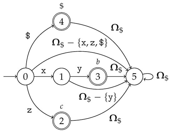
Figure 2.
The scanner automaton for the specification in (1).
Parsing the input string results in the GSS and the scanner trace presented in Figure 3 and Figure 4, respectively. The scanner trace outlines the paths through the scanner automaton for each recognized lexeme. The number above each start state is the position at which the automaton starts, and corresponds to from which the shift action will be performed. The terminal symbol above each final state is the lookahead symbol that is passed to the parser. When the automaton enters a dead state, it can no longer match anything; thus, the paths end at that point. Additionally, note that there is no , as there are no matches at position 1.

Figure 3.
The GSS constructed by the traditional parsing architecture using the specification in (1).
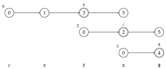
Figure 4.
The scanner trace outlining the paths taken through the scanner automaton using the specification in (1).
3.3. Context-Aware Scanning Architecture
Context-aware scanning [6,18] is an extension of the traditional parsing architecture. Likewise, the scanner automaton is constructed for the lookahead symbols . The difference is that the scanner is provided with the contextual information it lacks from the parser. The information is passed in the form of a valid lookahead set, which is a set of all lookahead symbols that are valid at a given point in the parse. The contextual information is summarized in the state of the handle-finding automaton; thus, for states , such a set can be constructed by collecting the lookahead symbols that have actions associated with them:
This limits the selection of automata that need to be considered at a given point; thus, for all , only a subset should be pairwise disjoint and pairwise prefix-disjoint . As a consequence, this allows more specifications to be parsed deterministically [6,18].
Let us define a function for as a reflexive transitive closure of m:
It returns the lookahead symbols that could possibly be matched by continuing from . The function can easily be defined for as . Note that, for a path , where , in the automaton, the following holds . In other words, the possibilities narrow as more of the input string is seen. As the automaton enters a dead state, , .
Conceptually, a context-aware scanner uses a distinct scanner automaton for each state in the handle-finding automaton , specialized for recognizing lookahead symbols in . There exist many different ways to construct such a scanner [6,7,8,9,18]. We use an approach proposed by Van Wyk [6] and Schwerdfeger [6,18].
Instead of constructing an automaton for each handle-finding automaton state, the same automaton is used as in the traditional parsing architecture, , and the scanning process is modified in a way that only lookahead symbols from can be recognized. The and are defined as:
In a traditional scanner, we know that an automaton can no longer match anything when it enters a dead state. Here, this is no longer the case, since we are interested in recognizing only a subset of possible lookahead symbols. Instead, we can use the alternative definition: For some , no more matches can be made from the state when . In other words, no lookahead symbols from could possibly be matched by continuing from . At that point, the automaton can be stopped. The automaton finds a match when , then is passed to the parser.
Note that, since possibilities narrow as more of the input string is seen, for a path , where we can use the following recursive definition as an optimization:
Since , we can instead use:
This way, the sets contain less lookahead symbols and the intersection is more efficient to compute [6,18].
The worst-case time complexity is , due to the fact that the intersection needs to be computed at each step. For any , initially ; however, the size of the sets decreases as possibilities narrow. The worst-case space complexity remains the same as for the traditional parsing architecture, , where is the number of states in the largest automaton; however, the size of the automata is increased by a constant factor due to the additional label on the states for p [18].
Let us combine RNGLR parsing and context-aware scanning. The combination was already suggested by Van Wyk [6] and Schwerdfeger [6,18], and is used by the Tree-sitter [34]. In RNGLR parsing, at each point in the parse, the handle-finding automaton may be in multiple states at once. The set of all possible combinations of these states for a given grammar can be defined as:
The valid lookahead set needs to be extended to each :
Conceptually, the context-aware scanner uses a distinct scanner automaton for each possible combination of handle-finding automaton states , specialized for recognizing lookahead symbols in .
The same idea is utilized, except that now is used instead. The functions and are defined as:
The worst-case time and space complexity remain unchanged.
There are no lexical conflicts if for all the automata corresponding to the lookahead symbols in are pairwise disjoint and pairwise prefix-disjoint; that is .
Let us define subsets of each subclass , where each represents the vertices created as the shift actions were processed at the previous position, and each of the following represents the vertices created after i reduce actions were processed, and n is the number of reduce actions processed in total. The corresponding sets of the handle-finding automaton states will be denoted as , where and . As identified by Van Wyk [6] and Schwerdfeger [6,18], the valid lookahead set for each state contains all lookahead symbols that can possibly follow at that position. That means that vertices created as a result of processing reduce actions cannot introduce any additional lookahead symbols; that is, . As a result, , where and . This allows us to construct the automaton and perform the scanning just once at each position in the parse . For this reason, we introduce automata used at each position in the parse , where:
The scanning process remains the same as in the traditional parsing architecture, only the scanner automaton is modified. As a demonstration, let us use the following specification as an example:
The handle-finding automaton, constructed using in (2), is presented in Figure 5, and the scanner automaton is presented in Figure 6. Recognizing the input string results in the GSS and the scanner trace in Figure 7 and Figure 8, respectively.
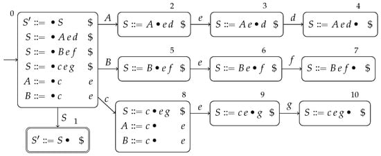
Figure 5.
The handle-finding automaton for the specification in (2), constructed using .
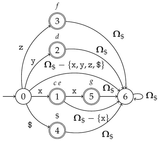
Figure 6.
The scanner automaton for the specification in (2).

Figure 7.
The GSS constructed by the context-aware scanning architecture using the specification in (2).

Figure 8.
The scanner trace outlining the paths taken through the scanner automaton using the specification in (2).
The valid lookahead sets for each handle-finding automaton state are and and and and and . They are used to determine the valid lookahead sets at each position based on the sets of states , both of which are given in Table 1.

Table 1.
The sets of states and the valid lookahead sets for the specification in (2).
Each row in the scanner trace represents the path traced by the automaton . At position 0, the scanning is performed using the automaton . The automaton starts in state 0, then a transition is performed.
Then a transition is performed.
At position 1, the scanning is performed using the automaton .
The automaton starts in state 0, then a transition is performed.
Then a transition is performed.
At position 2, the scanning is performed using the automaton . The automaton starts in state 0, then a transition is performed.
Then a transition is performed.
As already mentioned, context-aware scanning allows some of the specifications where the scanner automata are not pairwise disjoint or pairwise prefix disjoint, to be parsed deterministically. In this example, the languages of and are not disjoint, since they both match , which results in . However, there is no and , such that . This is easy to verify, . If that were not the case, there would be a lexical conflict. The possibility of such conflicts occurring was already identified by Tomita [15,16]; only a minor modification is required to the RNGLR parsing algorithm. The idea was later termed Schrödinger’s token by Aycock and Horspool [3]. In short, the algorithm performs the actions for all .
The languages of automata and are disjoint; however, they are not prefix-disjoint, since is a prefix of . There is again no and , such that . If that were not the case, there would be a lexical conflict. This type of lexical conflict is much harder to resolve since the recognized lexemes are of different lengths. The scanner would end up in two positions after matching . Subsequently, the scanner and the parser would need to split to handle both choices as proposed by Begel and Graham [14]. The same lexical conflict occurs if the languages of automata are not prefix-free. For example, the language , corresponding to exhibit this issue. This is usually resolved using the longest match disambiguation rule; however, this solution is not general. For example, the following specification cannot be parsed:
If we take a zoomed-out view of the GSS for in (2), focusing only on the shift actions, as presented in Figure 9, we can notice that there is a single path between any two subclasses. This is due to the fact that scanning has been completely deterministic up until this point. At each position , at most, one lexeme could be recognized, which corresponds to (at most) one lookahead symbol.
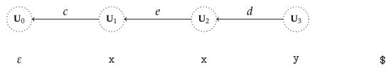
Figure 9.
Zoomed-out view of the GSS for the specification in (2) only displaying the edges resulting from shift actions.
In general, scanning is non-deterministic. Multiple automata can match the same lexeme, and/or multiple different lexemes can be recognized. Next, we present our extension of the context-aware scanning architecture and RNGLR parsing, which can handle the non-determinism efficiently.
4. RNGSGLR (0,1]
The algorithm presented in this section will be a recognizer. The lexical conflict resulting from multiple automata matching the same lexeme can already be resolved efficiently using Schrödinger’s token [3,15,16]. The problem we tackle is the lexical conflict resulting from recognizing multiple lexemes of different lengths.
Our architecture builds on context-aware scanning, likewise, we have the automata for each position in the parse. The difference is that we consider all possible lexemes matched by each . Let be a path traced by the automaton . We use to denote that the state belongs to and that it was entered at position . The state entered at position is the initial state; that is , and the state entered at position is the last state, a state from which no more matches can be made if the automaton has one or . Some of these states are final; the set of positions in which the automaton enters a final state is:
We consider all lexemes , for all , where each is a substring of that starts at and ends at , such that . Note that the start state is not considered, as there is no need to recognize the lexeme as it is trivially present at any position.
As a result, the automaton that started scanning at position must scan alongside automata that started scanning at previous positions. For this reason, the scanner automaton at position in the parse is defined as:
It is a runtime simulated union of automata . These started scanning at position and are now in state , as they already traced a path . The string is a prefix of the lexeme that the automaton is looking forward to recognize in the future. Each automaton is thus scanning for the not yet recognized suffix. This description is also trivially valid for the automaton added at position , which is in the start state. The scanner automaton state is composed out of the states of automata in the union at position .
The scanner automaton at position can also be defined recursively:
The scanner automaton at position 0 is initially just the automaton . At each position , the scanner automaton performs the transition on the character , becoming the automaton . The scanner automaton is constructed by adding the automaton in the runtime simulated union. The scanner automaton state contains the states of and additionally the start state for .
As the input string is traversed, the scanner automaton traces a path , where for all , . The set of positions where the scanner automaton enters a final state is:
Therefore, all possible lexemes , for all are considered. The lexemes can overlap arbitrarily. If they do not, our architecture degenerates to context-aware scanning.
The description given so far may seem infeasible, as defined, the number of states grows with the position in the parse. However, basic algebraic properties of the union, can be used as the optimization [2].
- Once no more matches can be made by the automaton, then , and the automaton can be removed from the union. Therefore, at each position , the automata, where are filtered out.
- If no matches were found at position , it immediately means , as no shift actions can be performed by the parser. As a result, ; therefore, . This allows the scanner to move uninterruptedly to the next match.
- It is possible that automata are duplicates . This happens if they are in the same state , and if they can match the same set of symbols . Such automata are merged, resulting in an automaton . It is crucial that both starting positions are preserved. An example of a specification that exhibits such duplication is:
These optimizations are not strictly required; even the most naive implementation always results in a correct parse, albeit, it invariably exhibits the worst-case behavior.
The functions and are defined as:
The position is added because the recognized lexeme , starts at position . That means the shift actions need to be performed from .
The scanning process remains very similar to the (traditional) context-aware scanning process. At each position in the parse, the scanner recognizes a string in the rest of the input string using the automaton , such that and . Note that the scanner stops only when a match is found at position . This is the same as in (traditional) context-aware scanning, except that multiple lexemes are recognized for each automaton , which enters the final state. Moreover, might not even be a lexeme. If the only lexeme that is recognized is , then our architecture degenerates to context-aware scanning for that portion of the input string. Each lexeme is recognized in steps. That means that the scanning for each lexeme is suspended and resumed for each match between the positions and . The recognizer is passed and . The process is then repeated for and using .
Thus far, we only covered our extension of context-aware scanning, so let us motivate the needed modifications to the RNGLR parsing with an example:
The handle-finding automaton, constructed using in (3), is presented in Figure 10, and the scanner automaton is presented in Figure 11. Notice that all are prefix-free, and are not prefix-disjoint. Recognizing the input string results in the GSS and the scanner trace in Figure 12 and Figure 13 respectively.

Figure 10.
The handle-finding automaton for the specification in (3), constructed using .
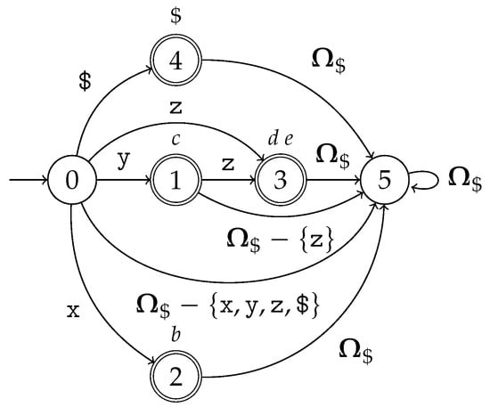
Figure 11.
The scanner automaton for the specification in (3).
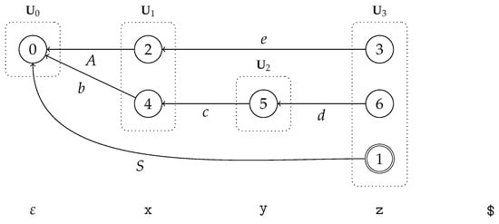
Figure 12.
The GSS constructed by our architecture using the specification in (3).

Figure 13.
The scanner trace outlining the paths taken through the scanner automaton using the specification in (3).
The valid lookahead sets for each handle-finding automaton state are and and and and . They are used to determine the valid lookahead sets at each position based on the sets of states , both of which are given in Table 2.
Table 2.
The sets of states and the valid lookahead sets for the specification in (3).
We start with , and scan until the first match , tracing a path . The scanning continues with to the next match , tracing a path . Now a reduce action can be performed; however, notice that the item has e as the lookahead symbol, which will be recognized in two steps. At this point, we already covered the first step; however, we still need to cover the second for e to be matched. We could scan ahead; however, this would mean the scanner and the parser would need to split. Instead, we choose to work with the information we have at this point. We can use , which tells us that we can still expect to match e and make the reduction based on this information. At worst, this means a superfluous reduction will be made, which will be ignored in the future. Since of the lexeme have been recognized, we call this approach the fractional lookahead. The automaton enters a dead state, so it can be removed. We continue scanning with to the next match , tracing a path The first thing to note is that . This lexical conflict occurs because does not hold. As already mentioned, this type of lexical conflict can be resolved by performing the actions for both e and d. In this case, a shift action is performed for both symbols. The second thing to note is that, to perform a shift action using e, it needs to be performed from . In traditional RNGLR parsing a shift action can only be performed from the previous subclass, which is ; therefore, the parsing algorithm needs to be modified. We continue scanning with to the next match , tracing a path . The reduce action is performed for S and parsing concludes successfully.
The scanner trace is a visual presentation of the path . The path is, in this case, concretely:
The scanner trace is not a data structure, at each point in the parse, only a single column is present in the memory. At each position , the column represents the state . At each position , the column without the added start state represents the state . The rows represent the paths traced by each . Note that traced the path , where . That is, the automaton entered the final state twice and two lexemes were recognized as a result. This occurred due to the fact that the lookahead symbols correspond to and , the languages of which are not prefix-disjoint since is a prefix of .
If we take a zoomed-out view of the GSS for in (3), focusing only on the shift actions, as presented in Figure 14, we can see that there can be more than one path between any two subclasses. The substring can be interpreted in two ways, either as e or c followed by d. In general, the shift actions alone now form a directed acyclic graph. The graph has a single path between any two subclasses exactly when our architecture degenerates to context-aware scanning.
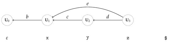
Figure 14.
Zoomed-out view of the GSS for the specification in (3) only displaying the edges resulting from shift actions.
The required modifications to the RNGLR parsing algorithm are:
- When more than one lookahead symbol is matched, , the actions are performed for all of them [3,15,16].
- At position , it must be possible to perform a shift action from any .
- The reduce actions are selected based on a prediction , if the entire lexeme is not recognized at position , which we call fractional lookahead.
The algorithm works as follows. At each position in the parse, a string is recognized using . Instead of a single lookahead symbol , there are now two sets of lookahead symbols, and . The set contains the lookahead symbols and the accompanying starting positions for shift actions. The set contains the lookahead symbols for the reduce actions. The lexemes for reduce actions can only start at position ; thus, the others are removed. Instead of just lookahead symbols that were matched, the set also contains those that can still be matched continuing from . This is essentially how the fractional lookahead is implemented. The vertices , such that are identified. The reduce actions are processed exactly as in RNGLR parsing. Then, for each the vertices , such that are identified. The shift actions are processed exactly as in RNGLR parsing. Then the process is repeated for and and . If there exists , such that , the parsing is completed successfully.
4.1. Support for Nullable RE
To support all possible , the case when , where , needs to be considered as well. That means the symbols can be nullable as well, . The solution is to use if when computing the sets. In the case of shift actions, the lookahead traditionally always coincides with the symbol to be shifted; thus, no special consideration is needed [1]. When the terminal symbols can be nullable, this is no longer the case. For each state , the shift items are converted into . The -shift actions need to be differentiated because they are performed within . The definition of valid lookahead sets remains the same. That means -shift actions must be considered as well.
The scanning process remains exactly the same. There is no need to recognize the lexeme as it is trivially present at any position . The parsing process needs to be modified as follows: The reduce actions are processed in the same way as before. Additionally, at each position in the parse, the vertices such that are identified. In the case of -shift actions for the vertex , a vertex is either found or created and the vertices are connected with an edge . The -shift actions are processed in exactly the same way as -reduce actions. Since -shift actions are performed within , this means new vertices can be created that need to be processed. For this reason, reduce and -shift actions are processed in a common loop until there are no possible actions left. The -shift actions can connect to an existent vertex , which was created as a result of a shift action starting from . Therefore, for all such , the reduce actions, where , must be processed before processing -shift actions. Otherwise, the reduction step will be applied twice, once using the short-circuiting reduce action from w or one of its descendants, and once more using a reduce action from . The shift actions are processed in the same way as before.
To demonstrate the required modifications, consider the following specification:
The handle-finding automaton, constructed using in (4), is presented in Figure 15, and the scanner automaton is presented in Figure 16. The handle-finding automaton results in the and presented in Table 3 and Table 4 respectively. The productions that are right nullable are and and . In contrast to RNGLR parsing [17], the nullable part can contain both terminals and non-terminals. The remains unmodified; however, it is still presented for completeness. Recognizing the input string results in the GSS and the scanner trace in Figure 17 and Figure 18, respectively.
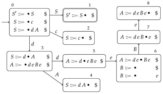
Figure 15.
The handle-finding automaton for the specification in (4), constructed using .

Figure 16.
The scanner automaton for the specification in (4).
Table 3.
The action table for the specification in (4).
Table 4.
The goto table for the specification in (4).
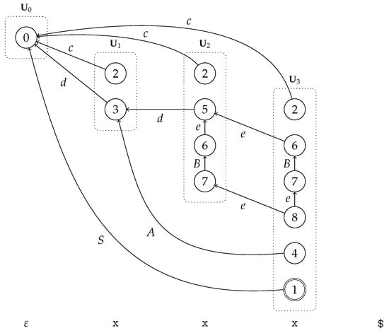
Figure 17.
The GSS constructed by our architecture using the specification in (4).

Figure 18.
The scanner trace outlining the paths taken through the scanner automaton using the specification in (4).
The valid lookahead sets for each handle-finding automaton state are and and and . The valid lookahead set for state 5 is a result of , since and . They are used to determine the valid lookahead sets at each position based on the sets of states , which in turn, are used to determine the sets and . These are given in Table 5.
Table 5.
The sets of states , the valid lookahead sets , and the sets and for the specification in (4).
In a short-circuiting reduce action is applied from state 6, and a reduce action is applied from state 8. An -shift action is applied from state 7 to state 8, adding an additional descendant. The reduce action from state 8 must be applied before the edge is created, otherwise both and are applied down the path . This formation occurs in the GSS, because there are two possible interpretations for , either the first e corresponds to and the second to , or vice versa.
If we take a zoomed-out view of the GSS for in (4), focusing only on the shift actions, as presented in Figure 19, in addition to there being multiple paths between any two subclasses, there are loops due to -shift actions.
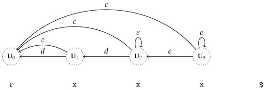
Figure 19.
Zoomed-out view of the GSS for the specification in (4) only displaying the edges resulting from shift actions.
4.2. Discussion
The solution is to perform all possible traversals of the scanner automata in addition to all possible traversals of the handle-finding automaton. In our architecture, the processes remain conceptually synchronized, all reduce actions are performed before shifting the next input symbols, and all the processes move to the next position at the same time. On top of that, the scanner automata remain synchronized as well, as they all scan the next character at the same time.
The fractional lookahead arises as a direct consequence of the requirement to preserve the synchronization. At position in the parse, when scanning using , it is likely that multiple matches can be found by . Moreover, it is entirely possible that the next match will instead be found by any of and not . We are aware of the following alternative solutions:
- Split the scanner and the parser; in that way, one part can remain at the current position and the other can continue with the scanning. This was proposed by Begel and Graham [14].
- Continue scanning, and when the matches are found, backtrack to the current position. This was conjectured by Keynes. This would be inefficient, due to repeated scanning and backtracking [8].
When either is used, the synchronization is lost. As already mentioned, in our case, no additional scanning is performed, which preserves the synchronization, and instead the reduce actions are selected based on the predictions made from the recognized prefix of the lexemes. In other words, only a fraction of the lexemes is recognized at this point. In the worst-case, , since at least one character must be scanned before a match is found. In the best case, is a lexeme. That happens when our architecture degenerates to context-aware scanning, and, in that case, the length of the lookahead is 1. In general, the length of the lookahead is a fraction , where , and is, therefore, on the interval . Note that the fraction varies based on which lexeme is considered; however, the value is always on the said interval.
Our architecture is flexible enough, in that the automaton from the traditional parsing architecture could be used directly. The problem is that, in the case of lexical conflicts, matches would be found at position , and then no shift actions could be performed using the corresponding lookahead symbols. As a result, the efficiency of the algorithm would be worse for the lexically ambiguous specifications. Additionally, superfluous matches would result in shorter and, thus, less lookahead.
A similar issue arises when using weaker handle-finding automaton construction algorithms, such as LALR or SLR [8]. In those cases, the valid lookahead sets can contain additional symbols that cannot result in a sentential form. That means an invalid match can be found in certain cases. An example of a specification that exhibits this issue when used in combination with LALR is:
If an invalid match is found at position , then . In RNGLR parsing, it is an indication that the parsing concluded unsuccessfully; however, in the case of our architecture, can still find a match. Therefore, parsing concludes unsuccessfully if and only if .
Lexical conflicts can occur at each position , for the same reasons as in context-aware scanning, and additionally if the languages of automata are not pairwise disjoint and pairwise prefix-disjoint.
The worst-case time complexity of our architecture is , where is the length of the longest right-hand-side of a production rule in the grammar. The reasons for this are as follows:
- There can be at most vertices in any , since each vertex is labeled with a distinct handle-finding automaton state.
- Each vertex can have at most successors. This is due to the fact that, in the worst-case, the handle-finding automaton can start searching for of some production rule , where , in each , and then perform reduction steps to the same vertex in .
- The number of steps required to find the paths of length , where and , is limited by the number of ways the intervening input symbols can be divided among symbols, . Summing over all possible final positions results in steps.
- The shift actions at position can be performed from any subclass . The can only contain vertices at most and actions can be performed for each vertex. Therefore, the shift actions are processed in steps.
- The automaton can be composed out of at most automata . In the worst-case, a match is found after scanning a single character , . Thus, steps are needed to perform the transitions on a for all of them. The worst-case time complexity of each is . Summing over all positions gives the worst-case time complexity of the scanner alone, .
- Each reduce action at position , in addition to the steps required to find the paths, requires at most steps, as the paths can end in at most vertices. The processing is, therefore, completely dominated by the search for the paths. The worst-case is when .
- The reduce actions at position are processed in steps. For each newly created vertex , in the worst-case, steps are required. For each edge , where , connected to an existing vertex w, in the worst-case, steps are required, as there is only one way to reach from w. In the worst-case , such connections can be made; therefore, steps are required in total.
- Summing over all positions gives .
However, usually , where . The recognizer performs and the scanner steps. Depending on the grammar, large segments of the input string can be processed by the scanner, and the recognizer is only involved when a match is found. The worst-case space complexity is , due to the size of the GSS. At each position , there can be at most vertices, and each vertex can have successors (edges). Summing over all positions gives [16,17,35]. The analysis is based on the analysis of GLR by Kipps; refer to [35] for additional rationale.
4.3. Algorithm
The scanning algorithm is very similar to the (traditional) context-aware scanning algorithm, except that at each position in the parse, is used as the scanner automaton and after it traces a path , both and are passed to the recognizer. We implement as a multi-map using and as keys:
That way, the automata that can no longer find a match can be filtered out and the duplicates can be merged while preserving the start positions.
The parsing algorithm will be presented in the imperative form. For this reason, we use mutable references to sets for the GSS and the subclasses . The presentation of the algorithm mainly follows that by Kipps [16,35] and Scott [17]. The actor is split into three functions actor, reduce_actor, shift_actor. Each one processes the actions directly by calling the corresponding processing functions reduce and shift. This allows us to specify precisely which additional actions need to be considered when a new vertex is added. In the parse function, we must first process the reduce actions, where , for vertices that are in at the start. Only then can -reduce and -shift actions be processed.
The multi-map maps the lookahead symbols t to vertices w, such that . There is one for each . They allow quick identification of the vertices in each subclass for which a shift action needs to be performed. These data structures are not strictly needed, since the vertices can be identified by just using ; however, a search is needed in that case. The worst-case space complexity of these data structures is , as there can be at most entries in each, and there is one at each position in the parse.
The algorithm listing is given in Algorithm 1. The input automata are just placeholders, as they are constructed at runtime. The real inputs are the automaton and a precomputed map .
| Algorithm 1. RNGSGLR(0,1] recognizer for character-level CFL. | |
| input | action table, goto table, automata at each position in the parse, |
| character input string | |
| output | accept or reject the character input string |
| let rngsglr1 = | |
| let rec actor w = | |
| if | |
| then shift w t | |
| if | |
| then | |
| for each do | |
| reduce w A 0 | |
| done | |
| and reduce_actor w = | |
| for each do | |
| for each successor node of w do | |
| reduce A | |
| done | |
| done | |
| and shift_actor () = | |
| for each match do | |
| for each do | |
| shift w l | |
| done | |
| done | |
| and reduce A = | |
| for each vertex v that can be reached from along the path of length , or length 0 if do | |
| let s = in | |
| if then | |
| add vertex u to labeled s and edge to | |
| actor u | |
| if | |
| then reduce_actor u | |
| else if then | |
| add edge to | |
| if then | |
| for each do | |
| reduce v B | |
| done | |
| and shift w t = | |
| let s = in | |
| if then | |
| add vertex u to labeled s and edge to | |
| if | |
| then actor u | |
| else if | |
| then add edge to | |
| in | |
| let parse () = | |
| scan at position in using tracing | |
| get matches | |
| get predictions | |
| for each vertex do | |
| reduce_actor w | |
| done | |
| for each vertex do | |
| actor w | |
| done | |
| shift_actor () | |
| construct | |
| in | |
| add the start vertex to labeled | |
| construct | |
| while do | |
| parse () | |
| done | |
| if | |
| then accept | |
| else reject | |
5. Construction of the Parse Forest
In this section, we extend the recognizer to a parser. To construct the parse forest, the following considerations are needed:
- The missing nullable parts must be added to the nodes produced by short-circuiting reduce actions [17].
- Multiple leaf nodes can be created at each point in the parse, since multiple lexemes can be recognized and each can correspond to multiple lookahead symbols.
We use an approach reminiscent of that of Scott [17], which, in turn, is based on that of Rekers [36].
The parsing algorithm finds all possible right-most derivations; therefore, multiple derivation trees can be constructed for a given sentence if the grammar is ambiguous. The construction of all individual derivation trees requires an exponential amount of work, and in certain cases might not terminate, even though the worst-case time complexity of the algorithm is polynomial [15,16]. The solution is to combine the common parts; that is, the subtrees are shared if multiple trees have a common subtree. If multiple nodes that correspond to the same non-terminal symbol have subtrees, which derive the same substring, then these nodes are merged into a single packed node. The resultant data structure is called a shared packed parse forest (SPPF) [16]. The SPPF is a variant of a directed graph, where each node can have multiple distinct sets of children (in the case of packed nodes). Each set of children is represented as a dot in the diagrams. Each node is labeled by a triple , such that and , where is a substring of the input string , starting at and ending at . For example, the SPPF for in (3) and is presented in Figure 20.
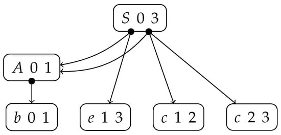
Figure 20.
The SPPF for the specification in (3) and .
The presence of nullable productions in the grammar may result in certain sentences having infinitely many derivations. As a result, and actions in those cases create cycles in the GSS, which, in turn, result in the cycles in the SPPF. The derivation trees can be recovered by unwinding the cycles [16,17]. An example of such a specification is in (5), which is presented further below.
There is a one-to-one correspondence between the edges in the GSS and the nodes in the SPPF. The construction is performed as follows: As a shift or an action corresponding to t is applied from the vertex , a vertex is either found or created. We search the SPPF for a node z labeled . If it does not exist, it is created. The vertices are connected with an edge , labeled z. The node corresponds to a lexeme . The lexemes should not be included in the nodes directly. Since they can overlap, their size can, in total, far exceed the size of the input string. As a reduce action corresponding to is applied from the vertex , the paths of length are found. As each path is traversed we record the labels on the edges, . For each a vertex is either found or created. We search the SPPF for a node z labeled in the case of actions, or in the case of reduce actions, where the node is labeled . If it does not exist, it is created. The nodes are then added as children to the node z if they are not already included. The vertices are connected with an edge labeled z [17,36]. In the case of right nullable productions , where , the subtrees corresponding to are missing from the SPPF, since the reduction steps are short-circuited [17]. To remedy this, Scott [17] pre-constructed the SPPF for of each right nullable production in the grammar, called the -SPPF. The nodes of the -SPPF are indexed, and the index is included in the reduce actions. As a short-circuiting reduce action is applied, a node from the -SPPF corresponding to the index is appended to the nodes of each path: . The -SPPF consists of nodes created using productions , where and terminal symbols . For this reason, -SPPF needs to be used when such nodes are created using -reduce or -shift actions, otherwise the nodes would be duplicated. Thus, the index of the -SPPF node needs to be included in each of these actions as well. The -SPPF nodes are just placeholders, and the appropriate SPPF nodes need to be inserted at their places after the GSS is constructed [17].
In our approach, we construct these SPPF nodes immediately. We include directly in the reduce actions, . To generate a subtree for all derivations of , where , we search the SPPF for a node z labeled . If it does not exist, it is created. For each , such that , where , we repeat the same process for all symbols , and add the resultant root nodes as children to node z. This requires us to pass the grammar to the parser; however, only productions , where are needed. Therefore, we can construct a trimmed-down version with only those productions. As a short-circuiting reduce action is applied, we generate the subtrees for all symbols corresponding to all derivations of , and the resultant root nodes are appended to the nodes of each path: . No modifications are required to the processing of -shift and -reduce actions, as the nodes from SPPF are reused when generating the subtrees. The benefit of our approach is that the SPPF is constructed to completion at each point during parsing. The downside is that the tables are slightly larger since the reduce actions additionally include a string instead of a single index. However, since the worst-case time complexity of RNGLR parsing depends on the lengths of the right-hand sides, we can expect these strings to be reasonably short. Despite the fact that the construction process is not exactly the same as that of Scott [17], the resulting SPPF is structurally equivalent. Therefore, our architecture can be used as a drop-in replacement for RNGLR in combination with (traditional) context-aware scanning.
Let us demonstrate the SPPF construction with the following example:
which corresponds to the following trimmed-down the grammar of nullable productions :
and the and given in Table 6 and Table 7 respectively.
Table 6.
The action table for the specification in (5).
Table 7.
The goto table for the specification in (5).
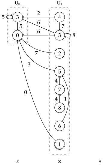
Figure 21.
The GSS constructed by our architecture using the specification in (5).

Figure 22.
The SPPF for the specification in (5) and .
The edges in the GSS are labeled with the indices of the SPPF nodes. All productions in the grammar are right-nullable. The short-circuiting reduce actions are applied in . and are applied in state 3. The subtrees corresponding to and are generated, resulting in the SPPF nodes 7 and 8. and are applied in state 5. The subtrees corresponding to and are generated, resulting in the SPPF nodes 1 and 4.
The sets of states , the valid lookahead sets , and the sets and for each position are given in Table 8.
Table 8.
The sets of states , the valid lookahead sets , and the sets and for the specification in (5).
Two lookahead symbols d and e are matched at position 0. An -shift action is performed from states 0 and 3. The resultant SPPF node is, in both cases, labeled ; thus, the edges share the index 5. For d, a shift action is performed from states 0 and 3, resulting in nodes labeled ; thus, the edges again share the index 6. For e, a shift action is performed from state 0, resulting in a node labeled and an edge labeled with index 3. There are infinitely many derivations for , since and . In our example, one d corresponds to and results in the SPPF node 6, while all others correspond to and result in SPPF nodes 5 and 8, and there can be infinitely many of them; hence, the loops in nodes 2 and 7.
Algorithm
The modifications required to generate the SPPF are purely additive. The algorithm listing is given in Algorithm 2. The algorithm now additionally accepts the trimmed-down grammar as an argument. The action processing functions shift and reduce are augmented to construct the SPPF nodes and label the edges. The shift now additionally accepts the start position of the lexeme, which is used as the start position of a leaf SPPF node. The function reduce now accepts the first edge of the path instead of just the successor vertex, because the SPPF node that labels this edge needs to be recorded as well. The nullable part of the right nullable productions is passed as well. That is then processed by the generate, which generates the missing subtrees. As in the algorithm proposed by Scott [17], the set is introduced, which holds the SPPF nodes constructed at each position in the parse. Only the nodes in need to be considered when searching for existing SPPF nodes. The labels of the SPPF nodes in share the end position; thus, they could have been omitted [17]. Note that, in our case, the SPPF nodes resulting from and shift actions need to be added to as well, as more than one node can be created. If the parse succeeded, the root SPPF node, the one that corresponds to the input string , labels the edge between the start vertex and a vertex w labeled with the final state of the handle-finding automaton. The nodes resulting from superfluously applied actions cannot be reached from the root SPPF node and can be removed.
| Algorithm 2. RNGSGLR (0,1] parser for character-level CFL. | |
| input | action table, goto table, automata at each position in the parse, |
| trimmed-down grammar of nullable productions, character input string | |
| output | accept or reject the character input string and return the constructed SPPF |
| let rngsglr2 = | |
| let rec actor w = | |
| if | |
| then shift w t | |
| if | |
| then | |
| for each do | |
| reduce A 0 | |
| done | |
| and reduce_actor w = | |
| for each do | |
| for each successor node of w do | |
| reduce A | |
| done | |
| done | |
| and shift_actor () = | |
| for each match do | |
| for each do | |
| shift w a | |
| done | |
| done | |
| and reduce A = | |
| let rec generate X = | |
| if | |
| then z | |
| else | |
| create node z labeled | |
| for each do | |
| let = map generate over in | |
| add children to z | |
| done | |
| z | |
| done | |
| in | |
| let = map generate over in | |
| for each v that can be reached via along the path of length and the corresponding do | |
| if then | |
| create node z labeled | |
| add children to node z | |
| let s = in | |
| if then | |
| add vertex u to , labeled s, and edge to labeled z | |
| if | |
| then reduce_actor u | |
| else if then | |
| add edge to | |
| if then | |
| for each do | |
| reduce B | |
| done | |
| and shift w t = | |
| if then | |
| create node z labeled | |
| let s = in | |
| if then | |
| add vertex u to , labeled s, and edge to labeled n | |
| else if | |
| then add edge to labeled z | |
| in | |
| let parse () = | |
| scan at position in using tracing | |
| get matches | |
| get predictions | |
| for each vertex do | |
| reduce_actor w | |
| done | |
| for each vertex do | |
| actor w | |
| done | |
| shift_actor () | |
| construct | |
| in | |
| add the start vertex to labeled | |
| construct | |
| while do | |
| parse () | |
| done | |
| if then | |
| the node z labeling is the root of the forest | |
| remove nodes not reachable from z | |
| accept | |
| else reject | |
6. Scanner Lookahead
By default, our architecture does not require a buffer. All characters are processed one by one. While all matched lookahead symbols result in a shift action due to the contextual information passed to the scanner by the parser (when using the canonical LR or an equivalent handle-finding automaton construction algorithm), some are still performed superfluously. In the example for specification in (4), the shift actions are performed for the symbol c in , , and ; however, all but the last are superfluous. The issue is that $ could have potentially followed at positions 2 or 3, and there was no way to tell if that were the case, since only one character was processed at a time. In practice, this arises when parsing embedded sub-languages. A simple example is the following specification:
When parsing the input string , the symbol b will be matched at positions 1, 2, 3, because there is no way to tell whether the next character is ".
A modest extension to our architecture, which solves this problem, is the addition of the scanner lookahead [2]. Usually, when a multitude of matches is found, all except the last result in a superfluous shift action. Therefore, the use of the scanner lookahead is functionally similar to the longest match disambiguation rule. However, the longest match in certain circumstances results in an incorrect parse. As identified by Nawrocki [9], there is the longest match conflict between not necessarily distinct , where and and , when:
When parsing , if the longest match is used, is recognized by , and then an error is raised because does not match [9]. To detect if the longest match conflict can occur, it is enough to consider only the first character of , as the parse is bound to be incorrect as soon as scans a single character past without returning a match. There is a special case, where and and and :
When parsing , all possible interpretations, such as , need to be considered. When using the longest match, the only possible interpretation is . The longest match results in an incorrect parse if can find a match after enters a final state.
In the case of our architecture, it occurs if can find a match as has entered a final state.
- When using our architecture, this is, by default, always assumed to be true. Every matched symbol is passed to the parser.
- When using the longest match, this is always assumed to be false. The scanning continues with until it is about to enter a state from which no more matches can be made on the next transition.
- When using the scanner lookahead, a test is performed if that is the case. We could scan ahead using the automaton to see if it enters a state from which no more matches can be made and then continue scanning in this case. Since only continuing with the scanning results in an incorrect parse, we can always stop early and return the match to the parser. We present a variant that is equivalent to scanning a single character. We use a simple set membership test instead of scanning ahead. The match is passed to the parser only if the rest of the input string contains , such that . This is equivalent to one character of lookahead in a character-level parser.
To determine the lookahead characters automatically using we introduce a valid-lookahead-lookahead multi-map, , which is the set of lookahead symbols for each lookahead symbol in the valid lookahead set. We identified the following approaches to compute :
- The simplest involves using the lookahead sets in a handle-finding automaton constructed using two symbols of lookahead as proposed by Keynes [8]. For each state , the shift items are converted into , and the reduce items are converted to . The issue with this approach is that construction of automata using two symbols of the lookahead is inefficient, as also noted by Keynes [8]. Additionally, it computes indirectly. It needs to compute two tokens of lookahead per item, which we have no use for, and then collapse it. We did not manage to make this approach reasonably efficient for large grammars.
- An approach based on exploring the right context of each LALR(1) handle-finding automaton state manually is given by Nawrocki [9].
- We found an efficient approach that allows us to compute directly. We construct the LALR(1) handle-finding automaton by converting the LR(0) handle-finding automaton to SLR [1]. The method works by constructing a grammar where each symbol is enhanced with the state of the LR(0) handle-finding automaton. The lookahead is computed as the sets of the enhanced non-terminal symbols. The is computed as the sets of the enhanced terminal symbols. In a sense, the corresponds to the lookahead that would be used when performing the reduce action for the symbol . The downside of the method is that it is tied closely to the handle-finding automaton construction method.
The scanner lookahead multi-map is then computed as
For a set of handle-finding automaton states, is defined as
The and are redefined as:
The scanning process is then modified as follows: The input string is extended with . At each position in the parse a string is recognized in the rest of the input string using as usual, such that . Then we peek at the next character a, such that . If none of the matched symbols pass the test, then , and as a result, ; therefore, the scanning immediately continues with . Otherwise, and are passed to the parser and the scanning continues with .
7. Proof of Correctness
A recognizer is correct for a given specification if it accepts an input string , if and only if , and otherwise rejects it. First, we will prove if our architecture accepts , then .
Lemma 1.
For each vertex , where , there must also exist a vertex , such that , where , and there must exist an edge in the GSS.
Proof.
This follows trivially from the definition of the handle-finding automaton and the basic operation of the RNGLR parser [15]. □
Lemma 2.
For each edge , such that and , created using a shift action, .
Proof.
The shift action is performed if after traces a path . That means the match was found by the automaton , such that , and that . Since , which means that and . The automaton is a union automaton, which means it finds a match if any of the constitutive automata find a match. The only automaton where is , which means it must necessarily be the one that recognizes . Therefore, , and by definition of , . □
Lemma 3.
For each edge , such that and , created using an ε-shift action or an ε-reduce action, .
Proof.
An -shift action or -reduce action is only performed if . Since at any position, . □
Lemma 4.
For each edge , such that and , created using a reduce action, where , .
Proof.
We will prove the statement by induction. If the GSS does not contain any edges, the statement is trivially satisfied. If the statement holds for all of the edges in the GSS, then it must hold after has been added. The reduce action , where , is performed if there exists a path , where and and . For each , where and , . This statement holds for the edge :
- Due to Lemma 2, if it was created as a result of a shift action;
- Due to Lemma 3, if it was created as a result of an -shift or -reduce action; or
- Due to the induction hypothesis, if it was created as a result of a reduce action.
This exhausts all possible ways an edge can be created. The reduce action entry was added to the actions table because . That means , where , and as a result . □
Theorem 1.
For each edge , such that and , in the GSS, .
Proof.
An edge can only be created as a result of a shift, an -shift, an -reduce or a reduce action, where ; therefore, the statement holds due to Lemmas 2, 3, 4. □
Theorem 2.
If our architecture accepts ω then .
Proof.
If our architecture accepts , it means there must exist a vertex , such that . This implies . By Lemma 1, there must exist a vertex v, such that and an edge . By the definition of the handle-finding automaton, the only such vertex is . Therefore, there exists an edge , such that and . By Theorem 1, , therefore, [15]. □
Second, we will prove that if , then our architecture accepts . We will do so by showing that our architecture accepts exactly when a character-level RNGLR parser accepts using . The correctness of RNGLR was proven by Scott [17].
We will formulate the lookahead as the right context. The item right context is the grammar that describes the language of all strings that can follow an item in state . For an item of the form , which was added as a result of the -closure on an item of the form , a production is added to the grammar. Shifting over a symbol does not change the item right context; thus, for the items of the form and , a production of the form is added . The dot right context is grammar that describes the language of all strings that can follow the dot. The grammar is initially constructed in the same way as for the item’s right context. Then, for each item of the form , a production is added [1]. We assume the character-level RNGLR uses the whole right context as the lookahead; in that way, it cannot perform superfluous actions. Our architecture performs strictly worse in that regard.
To avoid confusion, the symbols that belong to RNGLR will be annotated with and those that belong to our architecture will be annotated with .
Lemma 5.
For all states and , if , where :
Proof.
We will prove the statement by induction. The base cases are the states and . We will prove the statement holds for the base case, again by induction. Initially, and . If we assume the statement holds trivially as the initial items exist for both and by the definition of the handle finding automaton. We will prove that, as the items are expanded using -closure, the statement still holds: By the induction hypothesis, there exist items and , where and , or there are no such items in and . If , the items are added for both and . That is because productions , such that , exist in both grammars, by the definition of . Moreover ; therefore, the statement continues to hold.
Therefore, the statement holds for the base case. We will prove that the statement still holds after new states and are added. Each state is created from an existing state and . By the induction hypothesis, there exist items and , where and , or there are no such items in and . If they exist, then a new state and an edge are created for and new states and are created for . Initially, there exist items and . if , no more items are added and the statement continues to hold. Otherwise, if , then the items are expanded using -closure. We can use the same reasoning for and , to show that the statement still holds for the created items. Therefore, the statement holds for all and . □
Corollary 1.
For all states and , when , the item right context and the dot right context coincide for both and :
This follows trivially from Lemma 5.
Lemma 6.
contains all paths labeled in , for all derivations .
Proof.
The are the configurations of the stack in LR parsing [1]. We will prove the statement by induction. The base cases are the empty paths starting at and , which exist by the definition of both recognizers. By the induction hypothesis, there are paths:
We will prove that if an edge , where , is added to , an edge is added to . In either algorithm, an edge can only be added by processing an action. We will show that, if an action is performed by a character-level RNGLR, it is also performed by our architecture.
- 1.
- A reduce action for production , such that and and , is performed using a character-level RNGLR if there exists a path , where and , such that and , and if the rest of the input matches , such that .By the induction hypothesis, there exists a path , where and , as well. By Lemma 5, and , therefore . That means . The reduce action is performed if after traces a path . That will happen if . Since , then by Corollary 1, , where and .Therefore, it is guaranteed that , where . Thus, the action is also performed by our architecture. The relevant parts of the resulting and are presented in Figure 23.

Figure 23.
The relevant part of after the reduce action is performed by the character-level RNGLR and the corresponding part of after the reduce action is performed by our architecture.
Figure 23.
The relevant part of after the reduce action is performed by the character-level RNGLR and the corresponding part of after the reduce action is performed by our architecture.

- 2.
- The conditions for performing an action by the character-level RNGLR and our architecture are the same as in 1, except in this case, and , as . The relevant parts of the resulting and are presented in Figure 24.

Figure 24.
The relevant part of after the -reduce action is performed by the character-level RNGLR and the corresponding part of after the -reduce action is performed by our architecture.
Figure 24.
The relevant part of after the -reduce action is performed by the character-level RNGLR and the corresponding part of after the -reduce action is performed by our architecture.

- 3.
- The conditions for performing a reduce action for production , such that and and , are the same as in 1.By the induction hypothesis, there exists a path , where . The path does not exist for , because ; therefore, . By Lemma 5, . Since t is a terminal symbol in , there exists a shift action . This means . The shift action is performed if after traces a path . That will happen if . The reduce action creates an edge , such that and , in , which means [15,17]. As a result, a match will necessarily be found for t and the action will also be performed by our architecture. Since , then by Corollary 1, , where and . Furthermore, , where . That means and , and it is guaranteed that a will be found in the rest of the input string. Therefore, the action will also be performed if the scanner lookahead is used. The relevant part of the resulting and are presented in Figure 25.

Figure 25.
The relevant part of after the reduce action is performed by the character-level RNGLR and the corresponding part of after the shift action is performed by our architecture.
Figure 25.
The relevant part of after the reduce action is performed by the character-level RNGLR and the corresponding part of after the shift action is performed by our architecture.

- 4.
- The conditions for performing an -reduce action , such that and and , are the same as in 1. By the induction hypothesis, there exists a path , where . The path does not exist for , because . By Lemma 5, . Since , there exists an -shift action . This means . The -shift action is performed if after traces a path . That will happen if . Since , where , then by Corollary 1, , where and and . Therefore, it is guaranteed that , where . Thus, the action is also performed by our architecture. The relevant part of the resulting and are presented in Figure 26.
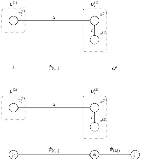 Figure 26. The relevant part of after the -reduce action is performed by the character-level RNGLR and the corresponding part of after the -shift action is performed by our architecture.
This exhausts all possible combinations of actions, where ; therefore, the statement holds for all paths . indeed contains all paths labeled in . □
Theorem 3.
If , then our architecture accepts ω.
Proof.
The (character-level) RNGLR algorithm accepts a string if there exists an edge in , such that and [15,17]. By Lemma 6, since is a path of length one, it exists in as well. By Theorem 2, our architecture accepts if such an edge exists. If , then the (character-level) RNGLR algorithm accepts as proven by Scott [17]. Our architecture accepts , if the character-level RNGLR algorithm accepts ; therefore, if then our architecture accepts . □
Traditionally, the parser is correct for a given specification if the constructed SPPF is a representation of all possible derivations, such that , where is a string of terminal symbols passed to the parser by the scanner. As a generalization, in our case, all possible are considered. Therefore, our architecture captures all lexical ambiguities.
Theorem 4.
The parser constructs the SPPF for all possible derivations , where and .
Proof.
This is easy to see from Lemma 6, our architecture constructs the GSS using containing all paths labeled in the GSS constructed by the character-level RNGLR using . The SPPF nodes are stored in the GSS edges and the construction of the SPPF nodes is equivalent as in the (character-level) RNGLR. The SPPF nodes , where , constructed by our architecture, are the same as the one constructed by the character-level RNGLR. The SPPF nodes , where , constructed by our architecture, are leaf nodes because t was recognized using the scanner. The same nodes constructed by the character-level RNGLR contain a subtree, created as a result of parsing t. Therefore, the SPPF constructed by our architecture is not exactly the same as the one for character-level RNGLR, the difference is that the subtrees for derivations are missing. □
8. Experience
As our architecture utilizes context-aware scanning [6,7] and the Schrödinger’s token [3,15,16] directly, it naturally supports all of the use cases of these techniques, and the interested reader should refer to [3,6,7]. It can also resolve trivially the conflicts that are reported to be difficult to resolve using these techniques alone. These difficulties arise due to conflicts of type (II), and are exactly the ones we aimed to resolve. We will assume the scanner lookahead is not utilized, otherwise, some of these conflicts are resolved even sooner. The [6] mentions a problem of scanning keywords (or operators) that are not pairwise-prefix disjoint, for example, and , appearing in C#. In the case of architecture, the automaton recognizes both keywords. After the shorter keyword is recognized and a shift action is performed, the said automaton continues scanning and recognizes the longer keyword if possible. In that case, the first shift action is performed superfluously. The [9] mentions a problem of recognizing as two integer numbers delimited by the range operator, instead of a floating-point number followed by a dot and a cardinal number, appearing in Pascal and Ada. In the case of architecture, the automaton recognizes both an integer and a floating-point number. After the integer number is recognized and a shift action is performed, an automaton is added, recognizing the range operator. After the floating-point number is recognized and a shift action is performed, no automaton would recognize the dot; therefore, this shift action was performed superfluously. After the range operator is recognized and a shift action is performed is added, again recognizing the integer or floating-point number. Note that our architecture can also handle the case where floating-point numbers are used in the range , which are not valid in Pascal or Ada. A similar case also occurs in COBOL, where the sentences conclude with a dot. Therefore, at the end of the sentence, should be regarded as an integer number, not a floating-point number. The [12,13] mentions a synthetic case where can be recognized either as a floating-point number or two integer numbers separated by a dot. In the case of our architecture, the automaton first recognizes an integer number. After that, an automaton that recognizes a dot is added, which is followed by an automaton that recognizes an integer number. The automaton continues scanning and recognizes the floating-point number as well. The use cases in most existing programming languages are all fairly trivial to resolve using our architecture and do not even come close to utilizing its full potential. The reason for this is that grammar writers have intentionally avoided introducing these conflicts due to the limitations of the traditional parsing architecture. Our architecture opens up new possibilities:
- Lexical syntax can vary arbitrarily for different parts of the programming language without carefully constructed scanner modes. All of the embedded sublanguages can be described in a single specification.
- During the development, thoughtless additions of regular expressions never result in an error, as our architecture accepts all possible specifications.
- A union, concatenation, and Kleene star of arbitrary specifications are invariably accepted, due to the closure properties of CFL, which allow for specifications to be composed.
- The transitions between different parts of the lexical syntax can be fluid, there is no need to surround them with sentinels. That means that multiple sublanguages can be possible in a certain context, and it can be left to the parser to determine which one it is parsing. For example, if we construct a specification that is a union of Pascal and C, the parser can determine if the input string contains Pascal or C.
- Capturing subpatterns in regular expressions are not required [37]. There is no need to treat parts of the lexical syntax as an opaque block and then extract certain parts out of it; in the case of our architecture, they can be treated as an embedded sublanguage.
- A simple error recovery resembling error tokens is supported without extensions, for example, where ; acts as a resynchronization token:
- When writing a specification with inserted white space, multiple types of white-space can be used, for example:Even if they both occur in the same context, it does not pose a problem.
This list is of course not exhaustive. The downside of our architecture is that while it can accept any possible specification, parsing can become slow when the number of possible interpretations becomes too large. The techniques developed to resolve this issue in the scannerless architectures [4,5,27,28,29] can be applied readily and we will consider adding them in future work.
9. Related Work
The related work can be grouped into scannerless and scanner-based methods. Our architecture can be categorized into the second group. The scanner-based methods can be deterministic or non-deterministic. The former used a variety of disambiguation rules to resolve the lexical conflicts in the scanner, and the latter offload the problem to the parser. How the methods are interrelated is shown in Figure 27.

Figure 27.
The dependency graph of the related work. Each is accompanied with the year of publication.
The earliest deterministic scanner-based method we are aware of is the work by Nawrocki [9]. Nawrocki categorized the types of lexical conflicts:
- The longest match conflicts, which are caused by the use of the longest match disambiguation rule.
- Identity conflicts, which are caused when the languages of the automata are not pairwise disjoint.
Additionally, lexical conflicts can occur when the languages of the automata are not prefix-free or pairwise prefix-disjoint, without causing the longest match conflicts. In that case, the longest match results in a correct parse. This was also identified by Denny [7]. Nawrocki presented two methods of resolving the lexical conflicts. The first one is called the left context , which is equivalent to an inverse of the valid lookahead . The second one is called the extended left context , which is equivalent to an inverse of the valid lookahead–lookahead . Because the functions are inverted, the tests and are performed instead of and , which is inconsequential. The is used in the same way as in the subsequent works. When the handle-finding automaton is in state s, the symbol is matched if . The method is used only if a single match is found in every state; that is when , . Otherwise, is used to disambiguate the matches further. The conflicts between for all are found as in (6). The method is used only if . When the handle-finding automaton is in state s, the symbol is matched if .
As identified by Denny [7] and to some extent by Keynes [8], the methods are limited. It is required that a single match is found in all handle-finding automaton states, otherwise, they cannot be used. This limitation can be lifted by further disambiguating the matched symbols using priority, as is done in context-aware scanning [6,18] and PSLR [7]. In the case of our architecture, no further disambiguation is needed.
They also cannot be used to decide when to pass a match to the parser. Let us demonstrate the problem with an example:
The longest match conflict only really occurs when the rest of the input string is . If the longest match disambiguation rule is used, would also recognize ∗ and an error would be raised. Therefore, a match must be passed to the parser beforehand. Just the information that a conflict is possible is useless in deciding when to pass the match to the parser. This was also identified by Denny [7], although the solution of additionally providing the shortest match disambiguation rule does not solve the problem.
We used as an optimization, which is equivalent to as already mentioned. We used it to construct the scanner lookahead . Because we used one character of the scanner lookahead, our method required a buffer of one character, exactly the same as the longest match disambiguation rule. Nonetheless, our method is able to resolve the problem in the specification (8). When ∗ follows in the rest of the input, a match is passed to the parser. Note that a match is also passed to the parser for each . This is not an issue, because, without the use of this optimization, the match is always passed.
Keynes [8] presents a deterministic architecture, which uses a scanner construction approach, where the labels m and p are stored in the edges, instead of the states. The construction is equivalent to first directly constructing the automata for each handle-finding automaton state. Additionally, each edge is labeled with the symbols that can be matched by starting again from the start state . Then, the lookahead symbols are removed if . That way, the scanner lookahead is incorporated into the automaton. That is possible because the labels are stored in the edges. The automata are then collapsed into a single automaton using minimization and a scanner mode is created for each of them. The scanner mode is then chosen based on the handle-finding automaton state. As noted by Keynes, the downside of the approach is that the construction method is inefficient [8]. Additionally, if we follow the disambiguation rules as given by Keynes, they cannot resolve the problem in (8). Keynes concludes that whether the matched symbol is passed to the parser or not is inconsequential as the conflict is unresolvable.
The PSLR by Denny [7] presents a deterministic architecture, which uses a scanner construction approach similar to the one used in context-aware scanning. Denny proposes a modified IELR handle-finding automaton construction method, which resolves the lexical conflicts that arise when weaker handle-finding automaton construction methods are used. The resulting handle-finding automaton has less states than the one constructed using LR(1). This would be the optimal method to use in combination with our architecture. However, it is not simple to implement; therefore, we used LALR instead.
Context-aware scanning by Van Wyk [6] and Schwerdfeger [6,18] presents the groundwork for our architecture. As already mentioned, our architecture degenerates to it when it is used for deterministic languages. We used the scanner construction approach described by Van Wyk [6] and Schwerdfeger [6,18]. Van Wyk and Schwerdfeger also suggest the architecture can be used in combination with GLR. The Tree-sitter [34] is an incremental parser generator based on this idea. However, just simply combining the approaches is not fully general.
The earliest non-deterministic method we are aware of is mentioned in the presentation of the GLR algorithm by Tomita [15,16]. As already mentioned, the lexical conflicts are treated as a parser conflict; therefore, the actions are performed for all matched symbols. The method was further discussed and termed Schrödinger’s token by Aycock and Horspool [3]. Our architecture can be viewed as a direct extension that additionally handles overlapping lexemes of different lengths. To maximize the time spent in the scanner and the length of lookahead, our architecture requires lexical feedback. As identified by Aycock and Horspool, this means that the phases cannot be parallelized. We agree that this is indeed a downside.
Keynes [8] conjectures a non-deterministic method termed generalized scanning. A generalized scanner would append the tokens to a list every time it enters a final state, and continue scanning until it enters a dead state. Then, the parser would process the tokens in the list, and the generalized scanner would move to the location of the match for the first token in the list and repeat the process. The generalized scanner would necessarily process characters multiple times in the case of lexical conflicts, and would require the entire string to be available in memory. Keynes noted that such an architecture would most likely be inefficient, and we agree with that assessment. Our architecture is a practical realization of the broader idea; for this reason, the GS in RNGSGLR stands for generalized scanning. It should be clear that our architecture does not actually work as conjectured by Keynes, as the parser “moves” with the scanner, and in that way the list is not required.
Character-level parsing was first proposed by Salomon and Cormack [4]. For this purpose, they extended the NSLR parser with exclusion and adjacency restriction disambiguation rules. NSLR is a non-canonical parser, which means that, in addition to terminal symbols, non-terminal symbols can be used as the lookahead when processing the reduce actions. Our architecture is similar in the sense that symbols in , which are used as lookahead, are non-terminal symbols in . The difference is that they are recognized by the scanner instead of the parser, and that in the case of lexical conflicts, they are only recognized partially, which we termed fractional lookahead. The exclusion rules implement the differences between the languages. In the case of our architecture, the difference is only available to the regular portion of the grammar in the form of extended regular expressions. The worst-case time complexity of the parser is , which is better than our architecture; however, it is not fully general, and for any given CFG, it cannot accept all corresponding character-level CFLs.
SGLR by Visser [5] is a character-level parser based on GLR. It uses the disambiguation rules introduced in character-level NSLR [4,5,38]. The parser is not non-canonical. Consequently, the reduction order is more predictable, although the worst-case complexity of the parser is the same as GLR and our architecture. This is the only other practical approach we are aware of that is fully general, and for any given CFG can accept all corresponding character-level CFLs. To parse , it instead parses the corresponding character-level CFG . Due to the use of exclusion rules in the context-free part of the grammar, it can also parse some of the context-sensitive languages. The downside of SGLR is that it uses a parser for the lexical portion of the grammar. As a result, the characters in the input string are processed multiple times—once when the shift action is performed and then again when (possibly) multiple reduce actions are performed and the parser searches for the paths passing the edge created by the shift action. In the case of our architecture, each character is processed exactly once. Since a parser is used as a scanner, the worst-case time complexity is , while, in the case of our architecture, it is . The lookahead in SGLR is a single character, while, in our case, it can be multiple characters. In the case of deterministic languages, the lookahead is the whole lexeme; therefore, the same as in deterministic parsing. We only used a single character of lookahead as the scanner lookahead. The original description of the SGLR parser uses the solution by Farshi [16,39] to parse -grammars. Since this solution is less efficient, the SRNGLR was developed by Economopoulos [11], which is instead based on RNGLR.
XGLR (by Begel and Graham [14]) is a non-deterministic architecture based on GLR that is the most closely related to ours. The scanner needs to be constructed manually. The grammar writer can provide multiple scanner modes. These are required to be lexically unambiguous. The scanner mode is then chosen based on the handle-finding automaton state. Whenever a lexical conflict is encountered the parser process is split, and each is associated with a scanner mode. That way, the parser processes end up in different positions when the lexemes are of different lengths [14]. Consequently, each character is processed multiple times, and the entire input string must be available in the memory. For example, if a regular expression is used in one of the modes, the rest of the input string will be traversed immediately by that parser. The others will then process the same characters again, as they follow it. In contrast, our scanner processes the characters one by one, and each is processed exactly once because the synchronization is preserved. The automaton recognizing runs alongside other automata until the end of the input string. Due to the fact that each parser process is associated with a scanner mode, this poses additional difficulties when they are later merged. The parsers also cannot share some of the data structures once they split [14]. Our architecture avoids this, as each character is processed exactly once and the synchronization is preserved. Because the parser processes are synchronized and the handle-finding automaton and the scanner states are not directly associated, no special considerations are needed when they are merged. The benefit of XGLR is that a whole lexeme is used as the lookahead, even when the grammar is heavily non-deterministic. Since XGLR uses the longest match disambiguation rule and scanner modes need to be provided manually, it is not fully general and for any given CFG cannot accept all corresponding character-level CFLs.
The LAMB and Fence by Quesada [12,13] is a non-deterministic architecture based on a chart parser that is able to resolve lexical conflicts in a similar way as a generalized scanner, as conjectured by Keynes [8]. The scanner is based on top-down regular expression recognizers, one for each terminal symbol. The recognizers are run one by one at each position , where . This means that, in the case of lexical conflicts, the characters are necessarily processed multiple times, and the entire input string must be available in the memory. For example, if a regular expression is used, the rest of the input string will be traversed from each position . The scanner has two variants. When using the first one, at each position the recognizers search for the longest match, the positions of the matches are recorded, and the scanner moves to the closest one. When using the second one, at each position , all possible matches are considered, and the recognizers are run at each position in the input string . To prevent duplicates, the scanner needs to keep track of tokens that are already found at each position in the input string. The worst-case time complexity of both variants is , the same as our architecture. However, the first one is not fully general and the second one always considers all interpretations as in (7), even when they are not possible; therefore, the complexity is bound to be even in the best case. The scanner generates a graph of all transitions, which is passed to the parser, where it is used to initialize the chart and the parsing commences. The input string is traversed fully by the scanner before the parsing takes place. That means the passes are completely disjoint; therefore, contextual information cannot be passed from the parser to the scanner. As a result, some of the traversals must be discarded immediately by the parser. That only occasionally happens when our architecture is used in combination with weaker handle-finding automaton construction methods, such as LALR and SLR.
The parser by Borsotti [40] is an extension of GLR that can parse the extended CFGs directly, without first translating them to CFGs. It would seem that such a parser could parse the lexical part of the grammar as well; however, this is not the case. This was also identified by the authors who stated that the parser should be used in combination with the traditional parsing architecture [40]. The parser works by constructing an automaton for each right-hand-side of the production, which is then combined into the handle-finding automaton. The handle-finding automaton also includes links in the reverse direction. When performing the reduce actions the search for the paths in the GSS is performed by following these links. Consequently, each character would be processed multiple times, once when performing the shift action, and then again when performing (possibly) multiple reduce actions.
The faster GLR parsing by Aycock and Horspool [1,41] and the generalized regular (GR) parsing by Johnstone and Scott [42] are similar to our architecture in that they improve the performance of GLR parsing using an automaton. The parsers can be used at the character level, and for any given CFG, accept all corresponding character-level CFLs (the same as our architecture). These parsers do not perform shift and reduce actions as is customary with LR parsing. Instead, the parsing process is driven mostly by the automaton and the stack is used similar to the call stack for subroutines. When searching for a non-terminal symbol, the next state is pushed on the stack, and when the non-terminal symbol is recognized, and the parser continues from the popped state. As the use of the stack is reduced, these parsers are efficient; however, as a trade-off, the automaton is prohibitively large. Our architecture completely avoids the use of the stack for the lexical syntax, otherwise it functions similar to the RNGLR parser. That way, the tables for the parser are almost the same as in RNGLR parsing and the tables for the scanner are the same as in context-aware scanning.
10. Conclusions
In this paper, we presented a novel scanner-based architecture, which, for any given CFG accepts all corresponding character-level CFLs. Our architecture lifts the restrictions of the existing scanner-based methods. It does not require any disambiguation rules for resolving lexical conflicts. However, as our architecture captures all lexical ambiguities for certain applications, disambiguation rules are still useful to limit the number of interpretations. It can directly parse all possible specifications consisting of a grammar and regular definitions. As a result, the grammar writers are not restricted to grammars where the lexical syntax can be resolved deterministically. Grammars are also easier to modify because they are not dependent on a careful selection of disambiguation rules to be parsed. Conceptually, our architecture has an unbounded parser and scanner lookahead. Our architecture is streaming, which means the characters are processed one by one and do not require a buffer.
In future work, we will attempt to incorporate the scanner lookahead into the automata, following Keynes [8], as we expect it to be more efficient. To limit the number of possible interpretations and ease the development of specifications, we will consider adding the adjacency restriction disambiguation rule [4,5,38]. We might consider other extensions, such as conjunctive and Boolean grammars, as well [43]. Our architecture can currently process symbols as they are typed at the end of the input string. Inserting them in the middle or at the beginning is currently not supported. We will attempt to create an incremental version of our architecture, which will support insertions anywhere in the input string. Our architecture could be adapted to other parsing methods that have the same power as GLR, such as GLL [44]. Since our architecture can parse any specification, it can be useful for applications where the specifications are generated procedurally, such as grammar synthesis [45]. We will also extend our metalanguage to support some of the use cases of our architecture better. That is, following [5,6,22], we will enable composing, embedding, and extending specifications.
Author Contributions
Conceptualization, Ž.L.; methodology, Ž.L., M.Č., M.M. and T.K.; software, Ž.L.; validation, M.Č., M.M. and T.K.; formal analysis, Ž.L.; writing—original draft preparation, Ž.L., M.Č., M.M. and T.K.; writing—review and editing, Ž.L., M.Č., M.M. and T.K.; visualization, Ž.L.; supervision, M.M. and T.K. All authors have read and agreed to the published version of the manuscript.
Funding
The authors acknowledge the financial support from the Slovenian Research Agency (Research Core Funding No. P2-0041).
Institutional Review Board Statement
Not applicable.
Informed Consent Statement
Not applicable.
Data Availability Statement
Not applicable.
Conflicts of Interest
The authors declare no conflict of interest.
References
- Grune, D.; Jacobs, C.J.H. Parsing Techniques; Springer: Berlin/Heidelberg, Germany, 2008. [Google Scholar]
- Aho, A.V.; Lam, M.S.; Sethi, R.; Ullman, J.D. Compilers: Principles, Techniques, and Tools, 2nd ed.; Pearson Education: London, UK, 2006. [Google Scholar]
- Aycock, J.; Horspool, N.R. Schrödinger’s token. Softw. Pract. Exp. 2001, 31, 803–814. [Google Scholar] [CrossRef]
- Salomon, D.J.; Cormack, G.V. Scannerless NSLR(1) parsing of programming languages. In Proceedings of the ACM SIGPLAN 1989 Conference on Programming Language Design and Implementation, Portland, OR, USA, 19–23 June 1989; Wexelblat, R.L., Ed.; ACM: New York, NY, USA, 1989; Volume 24, pp. 170–178. [Google Scholar]
- Visser, E. Scannerless Generalized-LR Parsing; Technical Report; University of Amsterdam, Programming Research Group: Amsterdam, The Netherlands, 1997. [Google Scholar]
- Van Wyk, E.R.; Schwerdfeger, A.C. Context-aware scanning for parsing extensible languages. In Proceedings of the GPCE’07—Proceedings of the Sixth International Conference on Generative Programming and Component Engineering, Salzburg, Austria, 1–3 October 2007; Consel, C., Lawall, J., Eds.; ACM: New York, NY, USA, 2007; pp. 63–72. [Google Scholar]
- Denny, J.E. PSLR(1): Pseudo-Scannerless Minimal LR(1) for the Deterministic Parsing of Composite Languages. Ph.D. Thesis, Clemson University, Clemson, SC, USA, 2010. [Google Scholar]
- Keynes, N. Better Parsing Through Lexical Conflict Resolution. Unpublished Thesis. Available online: http://www.deadcoderemoval.net/files/honours-thesis.pdf (accessed on 4 March 2022).
- Nawrocki, J.R. Conflict detection and resolution in a lexical analyzer generator. Inf. Process. Lett. 1991, 38, 323–328. [Google Scholar] [CrossRef]
- Dejanović, I. Parglare: A LR/GLR parser for Python. Sci. Comput. Program. 2022, 214, 102734. [Google Scholar] [CrossRef]
- Economopoulos, G.; Klint, P.; Vinju, J. Faster scannerless GLR parsing. In Proceedings of the International Conference on Compiler Construction, York, UK, 22–29 March 2009; Franke, B., Ed.; Springer: Berlin/Heidelberg, Germany, 2009; Volume 24, pp. 126–141. [Google Scholar]
- Quesada, L.; Berzal, F.; Cortijo, F.J. A lexical analyzer with ambiguity support. In Proceedings of the International Conference on Software and Data Technologies, Seville, Spain, 18–21 July 2011; pp. 297–300. [Google Scholar]
- Quesada, L.; Berzal, F.; Cortijo, F.J. Fencing the lamb: A chart parser for modelCC. In Proceedings of the Software and Data Technologies, Rome, Italy, 24–27 July 2012; Cordeiro, J., Hammoudi, S., van Sinderen, M., Eds.; Springer: Berlin/Heidelberg, Germany, 2012; Volume 27, pp. 21–35. [Google Scholar]
- Begel, A.; Graham, S.L. XGLR: An algorithm for ambiguity in programming languages. Sci. Comput. Program. 2006, 61, 211–227. [Google Scholar] [CrossRef][Green Version]
- Tomita, M. Efficient Parsing for Natural Language; Springer: Berlin/Heidelberg, Germany, 1986. [Google Scholar]
- Tomita, M. (Ed.) Generalized LR Parsing; Springer: Berlin/Heidelberg, Germany, 1991. [Google Scholar]
- Scott, E.; Johnstone, A. Right nulled GLR parsers. ACM Trans. Program. Lang. Syst. 2006, 28, 577–618. [Google Scholar] [CrossRef]
- Schwerdfeger, A.C. Context-Aware Scanning and Determinism-Preserving Grammar Composition, in Theory and Practice. Ph.D. Thesis, University of Minnesota, Minneapolis, MN, USA, 2010. [Google Scholar]
- Baxter, I.D.; Pidgeon, C.; Mehlich, M. DMS: Program transformations for practical scalable software evolution. In Proceedings of the 26th International Conference on Software Engineering, Edinburgh, UK, 23–28 May 2004; Titsworth, F., Ed.; IEEE: Los Alamitos, CA, USA, 2004; pp. 625–634. [Google Scholar]
- Owens, S.; Reppy, J.; Turon, A. Regular-expression derivatives re-examined. J. Funct. Program. 2009, 19, 173–190. [Google Scholar] [CrossRef]
- Régis-Gianas, Y.; Jeannerod, N.; Treinen, R. Morbig: A Static parser for POSIX shell. J. Comput. Lang. 2020, 57, 100944. [Google Scholar] [CrossRef]
- Schwerdfeger, A.C.; Wyk, E.R.V. Verifiable composition of deterministic grammars. In Proceedings of the 30th ACM SIGPLAN Conference on Programming Language Design and Implementation, Dublin, Ireland, 15–21 June 2009; Hind, M., Diwan, A., Eds.; ACM: New York, NY, USA, 2009; Volume 44, pp. 199–210. [Google Scholar]
- Mernik, M.; Heering, J.; Sloane, A.M. When and how to develop domain-specific languages. ACM Comput. Surv. (CSUR) 2005, 37, 316–344. [Google Scholar] [CrossRef]
- Dageförde, J.C.; Kuchen, H. A compiler and virtual machine for constraint-logic object-oriented programming with Muli. J. Comput. Lang. 2019, 53, 63–78. [Google Scholar] [CrossRef]
- Mernik, M. An object-oriented approach to language compositions for software language engineering. J. Syst. Softw. 2013, 86, 2451–2464. [Google Scholar] [CrossRef]
- Fister, I.; Kosar, T.; Fister, I.; Mernik, M. EasyTime++: A case study on incremental domain-specific language development. Inf. Technol. Control. 2013, 42, 77–85. [Google Scholar] [CrossRef][Green Version]
- Van den Brand, M.; van Deursen, A.; Heering, J.; de Jong, H.; de Jonge, M.; Kuipers, T.; Klint, P.; Moonen, L.; Olivier, P.; Scheerder, J.; et al. The Asf+Sdf Meta-Environment: A Component-Based Language Development Environment. Electron. Notes Theor. Comput. Sci. 2001, 44, 3–8. [Google Scholar] [CrossRef][Green Version]
- Kats, L.C.; Visser, E. The spoofax language workbench: Rules for declarative specification of Languages and IDEs. In Proceedings of the ACM International Conference on Object Oriented Programming Systems Languages and Applications, Reno/Tahoe, NV, USA, 17–21 October 2010; Association for Computing Machinery: New York, NY, USA, 2010; pp. 444–463. [Google Scholar]
- Klint, P.; van der Storm, T.; Vinju, J. RASCAL: A domain specific language for source code analysis and manipulation. In Proceedings of the 2009 Ninth IEEE International Working Conference on Source Code Analysis and Manipulation, Edmonton, AB, Canada, 20–21 September 2009; pp. 168–177. [Google Scholar]
- Ma, L.; Ren, H.; Zhang, X. Effective Cascade Dual-Decoder Model for Joint Entity and Relation Extraction. Unpublished Paper. Available online: https://arxiv.org/pdf/2106.14163 (accessed on 16 June 2022).
- Krausová, M. Prefix-free regular languages: Closure properties, difference, and left quotient. In Proceedings of the Mathematical and Engineering Methods in Computer Science, Znojmo, Czech Republic, 25–28 October 2012; Kotásek, Z., Bouda, J., Černá, I., Sekanina, L., Vojnar, T., Antoš, D., Eds.; Springer: Berlin/Heidelberg, Germany, 2012; Volume 7119. [Google Scholar]
- Redziejowski, R.R. From EBNF to PEG. Fundam. Inform. 2013, 128, 177–191. [Google Scholar] [CrossRef]
- Watson, B.W. A Taxonomy of Finite Automata Construction Algorithms; Technical Report; Eindhoven University of Technology: Eindhoven, The Netherlands, 1993. [Google Scholar]
- Brunsfeld, M. Tree-Sitter. Available online: https://tree-sitter.github.io/tree-sitter/ (accessed on 4 March 2022).
- Kipps, J.R. GLR parsing in time O(n3). In Generalized LR Parsing; Tomita, M., Ed.; Springer: Berlin/Heidelberg, Germany, 1991; pp. 43–59. [Google Scholar]
- Rekers, J.G. Parser Generation for Interactive Environments. Ph.D. Thesis, Universty of Amsterdam, Amsterdam, The Netherlands, 1992. [Google Scholar]
- Laurikari, V. NFAs with tagged transitions, their conversion to deterministic automata and application to regular expressions. In Proceedings of the Seventh International Symposium on String Processing and Information Retrieval, A Curuna, Spain, 27–29 September 2000; pp. 181–187. [Google Scholar]
- Brand, M.G.J.V.; Scheerder, J.; Vinju, J.J.; Visser, E. Disambiguation filters for scannerless generalized LR parsers. In Proceedings of the International Conference on Compiler Construction, Grenoble, France, 8–12 April 2002; Horspool, N.R., Ed.; Springer: Berlin/Heidelberg, Germany, 2002; pp. 143–158. [Google Scholar]
- Nozohoor-Farshi, R. GLR Parsing for ε-Grammers. In Generalized LR Parsing; Tomita, M., Ed.; Springer: Berlin/Heidelberg, Germany, 1991; pp. 61–75. [Google Scholar]
- Borsotti, A.; Breveglieri, L.; Crespi Reghizzi, S.; Morzenti, A. Fast GLR parsers for extended BNF grammars and transition networks. J. Comput. Lang. 2021, 64, 101035. [Google Scholar] [CrossRef]
- Aycock, J.; Horspool, N.R. Faster generalized LR parsing. In Proceedings of the 8th International Conference, Amsterdam, The Netherlands, 22–28 March 1999; Jähnichen, S., Ed.; Springer: Berlin/Heidelberg, Germany, 1999; pp. 32–46. [Google Scholar]
- Johnstone, A.; Scott, E. Generalised regular parsers. In Proceedings of the 12th International Conference, Warsaw, Poland, 7–11 April 2003; Hedin, G., Ed.; Springer: Berlin/Heidelberg, Germany, 2003; pp. 232–246. [Google Scholar]
- Okhotin, A. Describing the Syntax of Programming Languages Using Conjunctive and Boolean Grammars. Unpublished Paper. Available online: https://arxiv.org/abs/2012.03538 (accessed on 10 March 2022).
- Van Binsbergen, L.T.; Scott, E.; Johnstone, A. Purely functional GLL parsing. J. Comput. Lang. 2020, 58, 100945. [Google Scholar] [CrossRef]
- Saffran, J.; Barbosa, H.; Pereira, F.M.Q.; Vladamani, S. On-line synthesis of parsers for string events. J. Comput. Lang. 2021, 62, 101022. [Google Scholar] [CrossRef]


Publisher’s Note: MDPI stays neutral with regard to jurisdictional claims in published maps and institutional affiliations. |
© 2022 by the authors. Licensee MDPI, Basel, Switzerland. This article is an open access article distributed under the terms and conditions of the Creative Commons Attribution (CC BY) license (https://creativecommons.org/licenses/by/4.0/).