A Primal–Dual Fixed-Point Algorithm for TVL1 Wavelet Inpainting Based on Moreau Envelope

Abstract

In this paper, we present a novel variational wavelet inpainting based on the total variation (TV) regularization and the l1-norm fitting term. The goal of this model is to recover incomplete wavelet coefficients in the presence of impulsive noise. By incorporating the Moreau envelope, the proposed model for wavelet inpainting can better handle the non-differentiability of the l1-norm fitting term. A modified primal dual fixed-point algorithm is developed based on the proximity operator to solve the proposed variational model. Moreover, we consider the existence of solution for the proposed model and the convergence analysis of the developed iterative scheme in this paper. Numerical experiments show the desirable performance of our method.

1. Introduction

As artificial intelligence technology developed, image inpainting became a key technique in image processing and computer vision [1,2]. The goal of image inpainting was to recover damaged or the missing information, either in the pixel domain or in the transformed domain or in both [3]. It has been extensively linked to other important tasks [4,5,6,7], like text and scratch removal, zooming and high-resolution image reconstruction, and impulsive noise removal, among many others. Up to now, a wide variety of image inpainting methods have been developed in the literature [8,9,10,11,12].

Generally, an image of size $n\times n$ is treated as a vector in $R^N$ (with $N=n^2$) by stacking up the columns of the image matrix. Let $\widehat{f}\in R^N$ be the acquired transformed coefficients with the missing ones set to zero and $\eta \in R^N$ be additive noise introduced in storage or transmission of the coefficients. Denoting by Ω the complete index set of transformed coefficients and $I\subset \mathrm{\Omega }$ as the index set of available ones, the image inpainting problem can be described as

$$f=MWu+\eta$$

(1)

where $W\in R^{N\times N}$ represents a transform matrix, $M\in R^{N\times N}$ is a diagonal matrix with $M_{ii}=1$ if $i\in I$ and $M_{ii}=0$ if $i\in \mathrm{\Omega }\backslash I$. The inpainting problem is to recover $u$ from $f$. The pioneering work in this area was proposed by Bertalmio et al. [11]. They have proposed a novel image inpainting model based on the nonlinear partial differential equations (PDE) of third order in image domain. Since then, a wide variety of image inpainting methods have been developed in the literature.

The follow-up studies show that the regularization functional-based method is a class of efficient techniques. In [6], Chan and Shen proposed the total variation (TV) inpainting model. Many methods have considered the curvature information along the isophote to realize the Connectivity Principle, including the curvature driven diffusion (CDD) by Chan and Shen [12] and the Euler elastic energy functional based model by Chan et al. [13]. Fuchs presented a comprehensive review on a class of higher order variational models related to the application in image inpainting [10]. However, these methods were all based on local geometrical information of an image, which were limited to non-texture images. Recently, a class of non-local methods has been extensively applied in image processing fields [14]. Moreover, Arias et al. [15] proposed a general variational framework for non-local image inpainting based on exemplar. Peyre et al. [16] also investigated the non-local TV for various image restoration problems, including the inpainting tasks. All these methods have been considered inpainting in the pixel domain.

In the JPEG2000 image compression standard, images are usually formatted and stored in terms of wavelet coefficients. Due to lossy transmission or communication, some damages to wavelet coefficients may heavily affect the image quality. The damaged regions in pixel domain cannot be well located and the degradation is often inhomogeneous. These prompt the need of recovering the damaged information in the wavelet domain. Chan et al. [3] have addressed this problem as wavelet inpainting, which corresponds to the problem (1) with $W$ being an orthogonal wavelet transform. Up to now, wavelet inpainting has received a lot of attentions [17,18,19,20,21,22]. Direct interpolation in the wavelet domain is problematic since high frequency coefficients retained cannot provide enough information for the missing ones. These motivate one to consider features in both the pixel domain and wavelet domain. Motivated by the idea of using TV minimization together with wavelet representation [23,24], Chan et al. [3] proposed the TV wavelet inpainting model. An objective function, which combines TV regularization term in the pixel domain with l²-norm fitting term in wavelet domain, is minimized to reproduce the damaged coefficients; we refer to this model as TVL2 model in this paper. They also have investigated some properties of this model, such as the existence and non-uniqueness of the solutions. Chan and Zhang extended the total variation wavelet inpainting to nonlocal total variation regularization [21]. The textures and local geometry structures are simultaneous when using this nonlocal method. Moreover, other regularization terms were introduced to overcome some drawbacks of the classical TV regularization, such as p-Laplace operator [19].

On the other hand, the fitting term plays an important to the variational model in the image processing. We can integrate the modified fitting term into the variational based wavelet inpainting for a specific purpose. Tai et al. [18] considered the sparsity of wavelet coefficients and proposed to combine TV regularization with l⁰-norm fitting in wavelet domain. In image restoration, theoretical and empirical analysis shows that the l²-norm fitting is less effective for handling the impulsive noise, while the l¹-norm fitting can effectively suppress the outliers occurring in images. Thus, the l¹-norm fitting is suitable for impulsive noise removal. Furthermore, it is well-known that the l¹-norm for image denoising does not erode the geometrical structures of the image. These observations motivate us to propose the TVL1 wavelet inpainting model, which combines the TV regularization with the l¹-norm fitting for the inpainting wavelet coefficients corrupted by impulsive noise. The difficulties are the non-differentiability of both the TV regularization and l¹-norm fitting.

Many numerical methods have been proposed to solve the TV-based problems, including time marching scheme, split Bregman/Augmented Lagrangian method and primal-dual method [1,22,25,26]. Recently, Micchelli et al. [27] proposed a fixed-point algorithm based on proximity operator (FP²O) to solve the total variation based denoising model. Inspired by the proximal forward–backward splitting (PFBS) [28] and the FP²O algorithm, Chen et al. [29] have proposed a primal–dual fixed-point algorithm based on proximity operator (PDFP²O) to minimize the sum of the TV regularization and a general differentiable fitting term. Liu et al. proposed a constrained second-order total generalized variational model for image denoising and utilized the primal–dual proximity method to solve it [30]. The non-differentiable fitting term makes it difficult to solve the variational model. Many researchers tackle this problem by introducing additional quadratic terms with some auxiliary variables [31,32]. As is pointed out in [33], this type of method could be included in the framework of Moreau envelope. In this paper, we utilize the Chen et al.’s algorithm and the Moreau envelope to solve the TVL1 wavelet inpainting model approximately and give the convergence analysis of the developed iterative scheme in the framework of the PDFP²O algorithm.

This paper is organized as follows. In Section 2, we present a brief introduction of the Moreau envelope (Section 2.1) and the PDFP²O algorithm (Section 2.2). We present the wavelet inpainting variational model based on the l¹-norm in Section 3.1, and its numerical scheme for the proposed model in Section 3.2. We present some numerical results for different kinds of images in Section 4. Finally, this paper is concluded in Section 5.

2. Background

In this section, we briefly review the Moreau envelope (Section 2.1) and the primal–dual fixed-point algorithm based on proximity operator (PDFP²O) (Section 2.2).

2.1. Moreau Envelope

Moreau envelope is used to smooth a non-smooth convex function. Let ${\mathrm{\Gamma }}_0(R^N)$ be the set of all proper lower semi-continuous convex functions $\psi :R^N\to (-\infty ,+\infty )$, such that the domain $dom(\psi ):=\{x\in R^N:\psi <+\infty \}$ of $\psi$ is nonempty. For $\mathsf{\Phi }\in {\mathrm{\Gamma }}_0(R^N)$, we denote its Moreau envelope of index $\alpha$ at $\nu \in R^N$ by

$$en{v}_{\alpha \mathsf{\Phi }}(\nu )=\min \left\{\mathsf{\Phi }(u)+\frac{1}{2\alpha }\Vert u-\nu {\Vert }_2^2:u\in R^N\right\}$$

(2)

The function $en{v}_{\alpha \mathsf{\Phi }}$ is still proper lower semi-continuous on $R^N$ and always differentiable with the gradient by

$$\nabla en{v}_{\alpha \mathsf{\Phi }}(●)=\frac{1}{\alpha }(I-pro{x}_{\alpha \mathsf{\Phi }})(●)$$

(3)

where $I$ is the identity operator from $R^N$ to $R^N$ and $pro{x}_{\mathsf{\Phi }}$ is the proximity operator of $\mathsf{\Phi }$ given by

$$pro{x}_{\mathsf{\Phi }}(\nu )=\arg \min \left\{\mathsf{\Phi }(u)+\frac{1}{2}\Vert u-\nu {\Vert }_2^2:u\in R^N\right\}$$

(4)

Moreover, the function $en{v}_{\alpha \mathsf{\Phi }}$ is bounded above by $\mathsf{\Phi }$ and converges pointwise to $\mathsf{\Phi }$ as $\alpha \to 0$ (Theorem 1.25 in [34]). The differentiability of Moreau envelope motivates one to smooth a non-smooth function by its Moreau envelope. For some $\mathsf{\Phi }\in {\mathrm{\Gamma }}_0(R^N)$, its proximity operator $pro{x}_{\mathsf{\Phi }}$ even has closed form.

For example, $\mathsf{\Phi }(●)=\alpha \Vert ●{\Vert }_1$ with $\alpha >0$. Let $y=pro{x}_{\mathsf{\Phi }}(\nu )$, then the i-th component of $y(i=1,2,\cdots ,N)$ is given by

$$y_i=\mathrm{sgn}({\nu }_i)\max \left\{|{\nu }_i|-\alpha ,0\right\}$$

(5)

where sgn is the sign function.

2.2. The PDFP²O Algorithm

Let $f_1\in {\mathrm{\Gamma }}_0(R^{2N})$, $f_2\in {\mathrm{\Gamma }}_0(R^N)$ and $f_2$ is differentiable on $R^N$ with a $1/\beta$-Lipschitz continuous gradient for some $\beta >0$. Many researchers pay more attention to an efficient algorithmic framework for the following minimization problem:

$$\underset{u}{\min }E(u)=f_1\circ B(u)+f_2(u)$$

(6)

where $B\in R^{2N\times N}$ is the first-order difference matrix defined as follow. $B\in R^{2N\times N}$ is described as

$$B=\left[\begin{array}{c}{I}_n\otimes D\\ D\otimes I_n\end{array}\right]$$

where $I_n$ is the identity matrix in $R^{n\times n}$, $D$ is the $n\times n$ matrix given by

$$B=\left[\begin{array}{ccccc}0& & & & \\ 1& 1& & & \\ & 1& 1& & \\ & & \ddots & \ddots & \\ & & & 1& 1\end{array}\right]$$

and the notation $U\otimes V$ denotes the Kronecker product of matrices $U$ and $V$. The problem (6) can be solved by the classical proximal forward–backward splitting algorithm, which can be shown by

$$\begin{array}{l}{u}^{*}=\underset{u}{\arg \min }{f}_1\circ B(u)+f_2(u)\\ 0\in \partial (f_1\circ B)(u^{*})+\nabla f_2(u^{*})\\ \iff -\nabla f_2(u^{*})\in \partial (f_1\circ B)(u^{*})\\ \iff u^{*}-\nabla f_2(u^{*})\in u^{*}+\partial (f_1\circ B)(u^{*})\\ \iff u^{*}={\left(I+\partial (f_1\circ B)\right)}^{-1}\left(I-\nabla f_2(●)\right)(u^{*})\end{array}$$

Thus, the problem (6) is equivalent to solving the fixed-point of operator ${\left(I+\partial (f_1\circ B)\right)}^{-1}\left(I-\nabla f_2(●)\right)(●)$. Inspired by the FP²O algorithm, Chen et al. [29] proposed a primal–dual fixed-point algorithm based on proximity operator (PDFP²O) as follows:

$$\left\{\begin{array}{l}{\nu }_{k+1}=(I-pro{x}_{\frac{\gamma }{s}}{f}_1)(B(u_k-\gamma \nabla f_2(u_k))+(I-sB{B}^T){\nu }_k)\\ u_{k+1}=u_k-\gamma \nabla f_2(u_k)-s{B}^T{\nu }_{k+1}\hspace{0.33em}\hspace{0.33em}\hspace{0.33em}\hspace{0.33em}\hspace{0.33em}\hspace{0.33em}\hspace{0.33em}\hspace{0.33em}\hspace{0.33em}\hspace{0.33em}\hspace{0.33em}\hspace{0.33em}\hspace{0.33em}\hspace{0.33em}\hspace{0.33em}\hspace{0.33em}\hspace{0.33em}\hspace{0.33em}\hspace{0.33em}\hspace{0.33em}\hspace{0.33em}\hspace{0.33em}\hspace{0.33em}\hspace{0.33em}\hspace{0.33em}\hspace{0.33em}\hspace{0.33em}\hspace{0.33em}\hspace{0.33em}\hspace{0.33em}\hspace{0.33em}\hspace{0.33em}\end{array}\right.$$

(7)

where the parameters $\gamma ,s>0$ and the variable $\nu$ could be understand as the dual variable of the primal dual formulation related to (6). The PDFP²O algorithm is convergent under some restrictions on the parameters $\gamma$ and $s$, which can be shown by Lemma 1 (Theorem in [29]). In this paper, we utilize the PDFP²O algorithm to solve the proposed model approximately.

Lemma 1.

Suppose $0<\gamma <2\beta$ and $0<s<1/{\lambda }_{\max (B{B}^T)}$ where ${\lambda }_{\max (B{B}^T)}$ is the largest eigenvalue of $B{B}^T$. Let $({\nu }_k,u_k)$ be a sequence generated by the iteration (7). Then the sequence converges $u_k$ to the minimizer of the problem (6).

3. The Proposed Model and Its Numerical Scheme

3.1. Wavelet Inpainting Variational Model Based on L1 Norm

Mathematically, image inpainting can be regarded as an ill-posed problem. This kind of problem can be solved by adding the regularization term into the variational model. Chan et al. [3] proposed the wavelet inpainting based on the total variation and the l²-norm (TVL2):

$$\underset{u}{\min }E(u)=\lambda \Vert u{\Vert }_{TV}+\frac{1}{2}\Vert MWu-\widehat{f}{\Vert }_2^2$$

(8)

where $\Vert u{\Vert }_{TV}=\Vert \nabla u{\Vert }_1$ refers to the total variation of the image, $\Vert ●{\Vert }_2$ is the l²-norm in $R^N$, and $\lambda >0$ is a scalar parameter balancing the TV regularization term and the fitting term. $\Vert u{\Vert }_{TV}$ plays the role of regularization, incorporating additional a priori knowledge into the problem to convert the ill-poised problem into a well-posed one or select one from the infinitely possible solutions. The fitting term based on l²-norm can be used to penalize inconsistency between the observed image and the estimated image. They perform well on some geometrical information and reduce Gaussian noise and other oscillations (e.g., Gibbs’ phenomenon). The experiments show that the TVL2 model can recover the missing wavelet coefficients, while preserving the geometrical features in pixel domain.

Impulsive noise often occurs in the storage or transmission of the coefficients. It could seriously affect the image quality. Thus, we should pay more attention to the impulsive noise in the processing of wavelet inpainting. The TVL2 model cannot provide desirable reconstruction result, which use the l²-norm fitting term. Many studies pay their attention to the l¹-norm fitting term. Thus, it is widely used for impulsive noise removal or deblurring or both due to its distinctive and desirable features such as the contrast and edge preservation, data driven scale selection and multiscale decomposition. This consideration motivates us to propose the following TVL1 model for wavelet inpainting:

$$\underset{u}{\min }E(u)=\lambda \Vert u{\Vert }_{TV}+\frac{1}{2}\Vert MWu-\widehat{f}{\Vert }_1$$

(9)

where $\Vert ●{\Vert }_1$ denotes the l¹-norm in $R^N$, $\lambda >0$ is a scalar parameter balancing the TV regularization and the fitting term. Thanks to the properties of the l1-norm fitting term, the TVL1 model can recover a good image from the partial wavelet coefficients corrupted by impulsive noise. The TVL1 model (9) can be reformulated as

$$\underset{u}{\min }E(u)=\varphi \circ B(u)+\mathsf{\Phi }\circ K(u)$$

(10)

where $\varphi (●)=\lambda \Vert ●{\Vert }_1:R^{2N}\to R$, $\mathsf{\Phi }(●)=\Vert ●-\widehat{f}{\Vert }_1:R^N\to R$, and $K=MW$. Due to the non-differentiability of the fitting term in (10), the TVL1 model for wavelet inpainting is not easy to solve. In the next subsection, the Moreau envelope is applied to tackling the non-differentiability of the l¹-norm, and then an iterative scheme based on the PDFP²O algorithm is presented, which is used to solve the associated problem.

3.2. Numerical Scheme for the Proposed Model

The main difficulty for the numerical treatment of the proposed model lies in non-differentiability of the fitting term. It is known that when the operator K in (10) is the identity operator in $R^{N\times N}$, this model becomes the TVL1 image denoising model. Various efficient numerical approaches have been proposed in the literature. However, all these approaches cannot be directly applied to solving the TVL1 model for wavelet inpainting.

Considering the non-differentiability of the function $\mathsf{\Phi }$ and the properties of the Moreau envelope, we substitute the function $\mathsf{\Phi }$ in (10) with its corresponding Moreau envelope. Then the modified TVL1 model is given as

$$\underset{u}{\min }{E}_{\alpha }(u)=\varphi \circ B(u)+en{v}_{\alpha \mathsf{\Phi }}(Ku)$$

(11)

where $\alpha >0$ is a scalar parameter determining how well the Moreau envelope approximates the function $\mathsf{\Phi }$ (a better approximation with a smaller $\alpha$). The following proposition shows the existence of a solution to the problem (11).

Proposition 1.

For each $\alpha >0$, let $\varphi$, $\mathsf{\Phi }$, $B$, $K$ be defined in (10), then the problem (11) has at least one solution.

Proof of Proposition 1.

By the definition of $en{v}_{\alpha \mathsf{\Phi }}$, we rewrite the problem as

$$\underset{u,\nu }{\min }{E^{\prime }}_{\alpha }(u,\nu )=\varphi \circ B(u)+\mathsf{\Phi }(\nu )+\frac{1}{2\alpha }\Vert Ku-\nu {\Vert }_2^2$$

(12)

Firstly, we show the existence of a minimizer to the function ${E^{\prime }}_{\alpha }$.

The first and second terms are obviously convex. The Hessian of

$$\Vert Ku-\nu {\Vert }_2^2=\Vert \left[\begin{array}{cc}K& 0\\ 0& -I_N\end{array}\right]\left(\begin{array}{c}u\\ v\end{array}\right){\Vert }_2^2$$

is given by

$$H=\left[\begin{array}{cc}{K}^{T}K& 0\\ 0& I_N\end{array}\right]=\left[\begin{array}{cc}{W}^{T}MW& 0\\ 0& I_N\end{array}\right]$$

where T is the transpose operator and $I_N$ is the identity matrix in $R^{N\times N}$. $H$ is a positive semidefinite since $M$ is positive semidefinite. Then ${E^{\prime }}_{\alpha }$ is convex. It is easy to see that ${E^{\prime }}_{\alpha }$ is proper and continuous. We only need to show that it is coercive, i.e., ${E^{\prime }}_{\alpha }(u,v)\to +\infty$ as $\Vert u{\Vert }_2+\Vert \nu {\Vert }_2\to +\infty$. We argue by its contrapositive. Let $\{(u_k,{\nu }_k)\}\subset R^N\times R^N$ be a sequence such that

$$\varphi \circ B(u_k)+\mathsf{\Phi }({\nu }_k)+\frac{1}{2\alpha }\Vert K{u}_k-{\nu }_k{\Vert }_2^2<+\infty$$

We deduce that

$$\varphi \circ B(u_k)<+\infty$$

(13)

and

$$\mathsf{\Phi }({\nu }_k)<+\infty$$

(14)

By Poincaré inequality, there exists a $C>0$ independent of $u_k$, so that

$$\Vert u_k{\Vert }_2^2\le C(\varphi \circ B(u_k))<+\infty$$

Moreover, (14) implies that $\Vert {\nu }_k{\Vert }_1\le \Vert {\nu }_k-\widehat{f}{\Vert }_1+\Vert \widehat{f}{\Vert }_1<+\infty$. Since ${\nu }_k\in R^N$ for any $k$, there exists a $C^{\prime }>0$ independent of ${\nu }_k$, so that

$$C^{\prime }\Vert {\nu }_k{\Vert }_2\le \Vert {\nu }_k{\Vert }_1<+\infty$$

Therefore, $\Vert u_k{\Vert }_2+\Vert {\nu }_k{\Vert }_2\to +\infty$. This shows the coercivity of $E_{\alpha }^{\prime }$. The existence of a minimizer to $E_{\alpha }^{\prime }$ follows.

Next, we show that if $(u^{\ast },{\nu }^{\ast })$ is a minimizer of $E_{\alpha }^{\prime }$, then ${\nu }^{\ast }=pro{x}_{\alpha \mathsf{\Phi }}(K{u}^{\ast })$. It directly follows that

$$E_{\alpha }^{\prime }(u^{\ast },{\nu }^{\ast })\le E_{\alpha }^{\prime }(u^{\ast },pro{x}_{\alpha \mathsf{\Phi }}(K{u}^{\ast }))$$

By the definition of proximity operator, we know that

$$\mathsf{\Phi }(v^{\ast })+\frac{1}{2\alpha }\Vert v^{\ast }-K{u}^{\ast }{\Vert }_2^2\ge \mathsf{\Phi }(pro{x}_{\alpha \mathsf{\Phi }}(K{u}^{\ast }))+\frac{1}{2\alpha }\Vert pro{x}_{\alpha \mathsf{\Phi }}(K{u}^{\ast })-K{u}^{\ast }{\Vert }_2^2$$

which together with the last inequality implies

$$\mathsf{\Phi }(v^{\ast })+\frac{1}{2\alpha }\Vert v^{\ast }-K{u}^{\ast }{\Vert }_2^2=\mathsf{\Phi }(pro{x}_{\alpha \mathsf{\Phi }}(K{u}^{\ast }))+\frac{1}{2\alpha }\Vert pro{x}_{\alpha \mathsf{\Phi }}(K{u}^{\ast })-K{u}^{\ast }{\Vert }_2^2$$

Hence, $v^{\ast }=pro{x}_{\alpha \mathsf{\Phi }}(K{u}^{\ast })$.

Finally, we show that if $(u^{\ast },{\nu }^{\ast })$ is a minimizer of $E_{\alpha }^{\prime }(u,v)$, then $u^{\ast }$ is a minimizer of $E_{\alpha }(u)$. Using the definition of the Moreau envelope, we have

$$en{v}_{\alpha \mathsf{\Phi }}(Ku)=\mathsf{\Phi }(pro{x}_{\alpha \mathsf{\Phi }}(Ku))+\frac{1}{2\alpha }\Vert pro{x}_{\alpha \mathsf{\Phi }}(Ku)-Ku{\Vert }_2^2$$

(15)

By (11), (12), and (15), we can obtain $E_{\alpha }^{\prime }(u,pro{x}_{\alpha \mathsf{\Phi }}(Ku))=E_{\alpha }(u)$. By contradiction, if $u^{\ast }$ is not a minimizer of $E_{\alpha }(u)$, then there exists a $u^{\prime }\in R^N$, such that $E_{\alpha }(u^{\prime })<E_{\alpha }(u^{\ast })$.

$$E_{\alpha }^{\prime }(u^{\prime },pro{x}_{\alpha \mathsf{\Phi }}(K{u}^{\prime }))=E_{\alpha }(u^{\prime })<E_{\alpha }(u^{\ast })=E_{\alpha }^{\prime }(u^{\ast },pro{x}_{\alpha \mathsf{\Phi }}(K{u}^{\ast }))$$

This inequality implies that $E_{\alpha }^{\prime }(u^{\prime },pro{x}_{\alpha \mathsf{\Phi }}(K{u}^{\prime }))<E_{\alpha }^{\prime }(u^{\ast },pro{x}_{\alpha \mathsf{\Phi }}(K{u}^{\ast }))$, which contradicts with the assumption that $(u^{\ast },{\nu }^{\ast })$ is a minimizer of $E_{\alpha }^{\prime }(u,v)$. This completes the proof. □

Many numerical methods have been proposed to solve the TV-based energy functional. In the following, we will utilize the PDFP²O algorithm to solve the proposed model (10) approximately. We have given a brief introduction to this algorithm in Section 2.2. Using Proposition 1, we obtain the numerical scheme for the modified model by the chain rule and the iteration scheme (7) as follows:

$$\left\{\begin{array}{l}{\nu }_{k+1}=(I-pro{x}_{\frac{\lambda \gamma }{s}\Vert ●{\Vert }_1})(B(u_k-\gamma K^T(\nabla en{v}_{\alpha \mathsf{\Phi }})(K{u}_k))+(I-sB{B}^T){\nu }_k)\\ u_{k+1}=u_k-\gamma K^T(\nabla en{v}_{\alpha \mathsf{\Phi }})(K{u}_k)-s{B}^T{\nu }_{k+1}\hspace{0.33em}\hspace{0.33em}\hspace{0.33em}\hspace{0.33em}\hspace{0.33em}\hspace{0.33em}\hspace{0.33em}\hspace{0.33em}\hspace{0.33em}\hspace{0.33em}\hspace{0.33em}\hspace{0.33em}\hspace{0.33em}\hspace{0.33em}\hspace{0.33em}\hspace{0.33em}\hspace{0.33em}\hspace{0.33em}\hspace{0.33em}\hspace{0.33em}\hspace{0.33em}\hspace{0.33em}\hspace{0.33em}\hspace{0.33em}\hspace{0.33em}\hspace{0.33em}\hspace{0.33em}\hspace{0.33em}\hspace{0.33em}\hspace{0.33em}\hspace{0.33em}\hspace{0.33em}\hspace{0.33em}\end{array}\right.$$

(16)

where $(u^{\ast },{\nu }^{\ast })$ is the transpose operator. Using the Formula (3) and the translation property of proximity operator, we have

$$\nabla en{v}_{\alpha \mathsf{\Phi }}(K{u}_k)=\frac{1}{\alpha }(I-pro{x}_{\alpha \mathsf{\Phi }})(K{u}_k)=\frac{1}{\alpha }(I-pro{x}_{\alpha \Vert ●{\Vert }_1})(K{u}_k-\widehat{f})$$

(17)

In (16) and (17), the proximity operator $pro{x}_{\rho \Vert ●{\Vert }_1}$ ($\rho =\alpha ,\lambda \gamma /s$) can be explicitly computed according to the Formula (5). For simplicity of description, we introduce an intermediate variable $u_{k+\frac{1}{2}}=u_k-\frac{\gamma }{\alpha }{K}^T(I-pro{x}_{\alpha \Vert ●{\Vert }_1})(K{u}_k-\widehat{f})$. By (17) and $u_{k+\frac{1}{2}}$, the iteration (16) can be changed into the iteration (18). The iterative of algorithm for the modified model (11) is summarized in Algorithm 1.

Algorithm 1 The numerical scheme for the proposed model

$$\begin{array}{l}\mathrm{Step}1.\mathrm{Given}{u}_0\in R^N,{\nu }_0\in R^{N\times N},\alpha >0,0<s<1/{\lambda }_{\max }(B{B}^T),0<\gamma <2\alpha ,tol>0\mathrm{is}\mathrm{a}\mathrm{tolerance}\\ \mathrm{Step}2.\\ \mathbf{while}\Vert u_{k+1}-u_k{\Vert }_2/\Vert u_k{\Vert }_2>tol\end{array}$$ $$\left\{\begin{array}{l}{u}_{k+\frac{1}{2}}=u_k-\frac{\gamma }{\alpha }{K}^T(I-pro{x}_{\alpha \Vert ●{\Vert }_1})(K{u}_k-\widehat{f})\hspace{0.33em}\hspace{0.33em}\hspace{0.33em}\hspace{0.33em}\hspace{0.33em}\hspace{0.33em}\hspace{0.33em}\\ {\nu }_{k+1}=(I-pro{x}_{\frac{\lambda \gamma }{s}\Vert ●{\Vert }_1})(B(u_{k+\frac{1}{2}}+(I-sB{B}^T){\nu }_k)\\ u_{k+1}=u_{k+\frac{1}{2}}-s{B}^T{\nu }_{k+1}\hspace{0.33em}\hspace{0.33em}\hspace{0.33em}\hspace{0.33em}\hspace{0.33em}\hspace{0.33em}\hspace{0.33em}\hspace{0.33em}\hspace{0.33em}\hspace{0.33em}\hspace{0.33em}\hspace{0.33em}\hspace{0.33em}\hspace{0.33em}\hspace{0.33em}\hspace{0.33em}\hspace{0.33em}\hspace{0.33em}\hspace{0.33em}\hspace{0.33em}\hspace{0.33em}\hspace{0.33em}\hspace{0.33em}\hspace{0.33em}\hspace{0.33em}\hspace{0.33em}\hspace{0.33em}\hspace{0.33em}\hspace{0.33em}\hspace{0.33em}\hspace{0.33em}\hspace{0.33em}\end{array}\right.(18)$$ end

In the following, we give the convergence analysis of the Algorithm 1 in the framework of the PDFP²O algorithm.

Proposition 2.

Suppose $0<\gamma <2\alpha$, and $0<s<1/{\lambda }_{\max }(B{B}^T)$, where ${\lambda }_{\max }(B{B}^T)$ is the largest eigenvalue of $B{B}^T$. Then the sequence $\left\{u_k\right\}$ generated by Algorithm 1 converges to a minimizer of the problem (11).

Proof of Proposition 2.

According to Lemma 1, it suffices to show that the composite function $en{v}_{\alpha \mathsf{\Phi }}\circ K$ is differentiable and its gradient is $1/\alpha$-Lipschitz continuous. By the chain rule and the differentiability of $en{v}_{\alpha \mathsf{\Phi }}$, it shows that $K^T\circ \nabla en{v}_{\alpha \mathsf{\Phi }}\circ K$ is $1/\alpha$-Lipschitz continuous.

In fact, for any $u_1$, $u_2\in R^N$, by Formula (16) we have

$$\begin{array}{l}{\Vert K^T⚬\nabla en{v}_{\alpha \mathsf{\Phi }}⚬K\left(u_1\right)-K^T⚬\nabla en{v}_{\alpha \mathsf{\Phi }}⚬K\left(u_2\right)\Vert }_2\\ =\frac{1}{\alpha }\Vert K^T⚬(I-{prox}_{\alpha \mathsf{\Phi }})⚬K\left(u_1\right)-K^T⚬(I-{prox}_{\alpha \mathsf{\Phi }})⚬K\left(u_2\right){\Vert }_2\\ \le \frac{1}{\alpha }{\Vert K^T\Vert }_2{\Vert (I-{prox}_{\alpha \mathsf{\Phi }})⚬K\left(u_1\right)-(I-{prox}_{\alpha \mathsf{\Phi }})⚬K\left(u_2\right)\Vert }_2\\ \le \frac{1}{\alpha }{\Vert K^T\Vert }_2{\Vert K\left(u_1\right)-K\left(u_2\right)\Vert }_2\\ \le \frac{1}{\alpha }{\Vert K^T\Vert }_2\Vert K{\Vert }_2{\Vert u_1-u_2\Vert }_2\\ =\frac{1}{\alpha }{\Vert W^T{M}^T\Vert }_2\Vert MW{\Vert }_2{\Vert u_1-u_2\Vert }_2\\ \le \frac{1}{\alpha }{\Vert W^T\Vert }_2{\Vert M^T\Vert }_2\Vert M{\Vert }_2\Vert W{\Vert }_2{\Vert u_1-u_2\Vert }_2\\ \le \frac{1}{\alpha }{\Vert u_1-u_2\Vert }_2\end{array}$$

where $\Vert K^T{\Vert }_2=\underset{u\in R^N,\Vert u{\Vert }_2=1}{\sup }\Vert K^{T}u{\Vert }_2$, which is similar for others. The first and third inequalities follow from the fact that both $K^T$ and $K$ are bounded linear operators, while the second inequality follows from the fact that $I-pro{x}_{\alpha \mathsf{\Phi }}$ is a firmly non-expansive operator [28] if $\mathsf{\Phi }\in {\mathrm{\Gamma }}_0(R^N)$. The last inequality holds due to $\Vert M^T{\Vert }_2=\Vert M{\Vert }_2=\rho (M)\le 1$ and $\Vert W^T{\Vert }_2=\Vert W{\Vert }_2=\sqrt{\rho (W^{T}W)}=1$, where $\rho (A)$ is the spectral radius of the matrix $A$. This completes the proof. □

Proposition 2 implies that, for a given $\alpha >0$, we can find a solution (denoted by $u^{\alpha }$) to the modified TVL1 model by Algorithm 1. Since

$$\underset{\alpha \to 0}{\lim }en{v}_{\alpha \mathsf{\Phi }}(Ku)=\mathsf{\Phi }(Ku),\mathrm{for}\mathrm{all}u\in R^N,$$

the solution of the modified model with a small enough $\alpha$ is a good approximate solution of the original model.

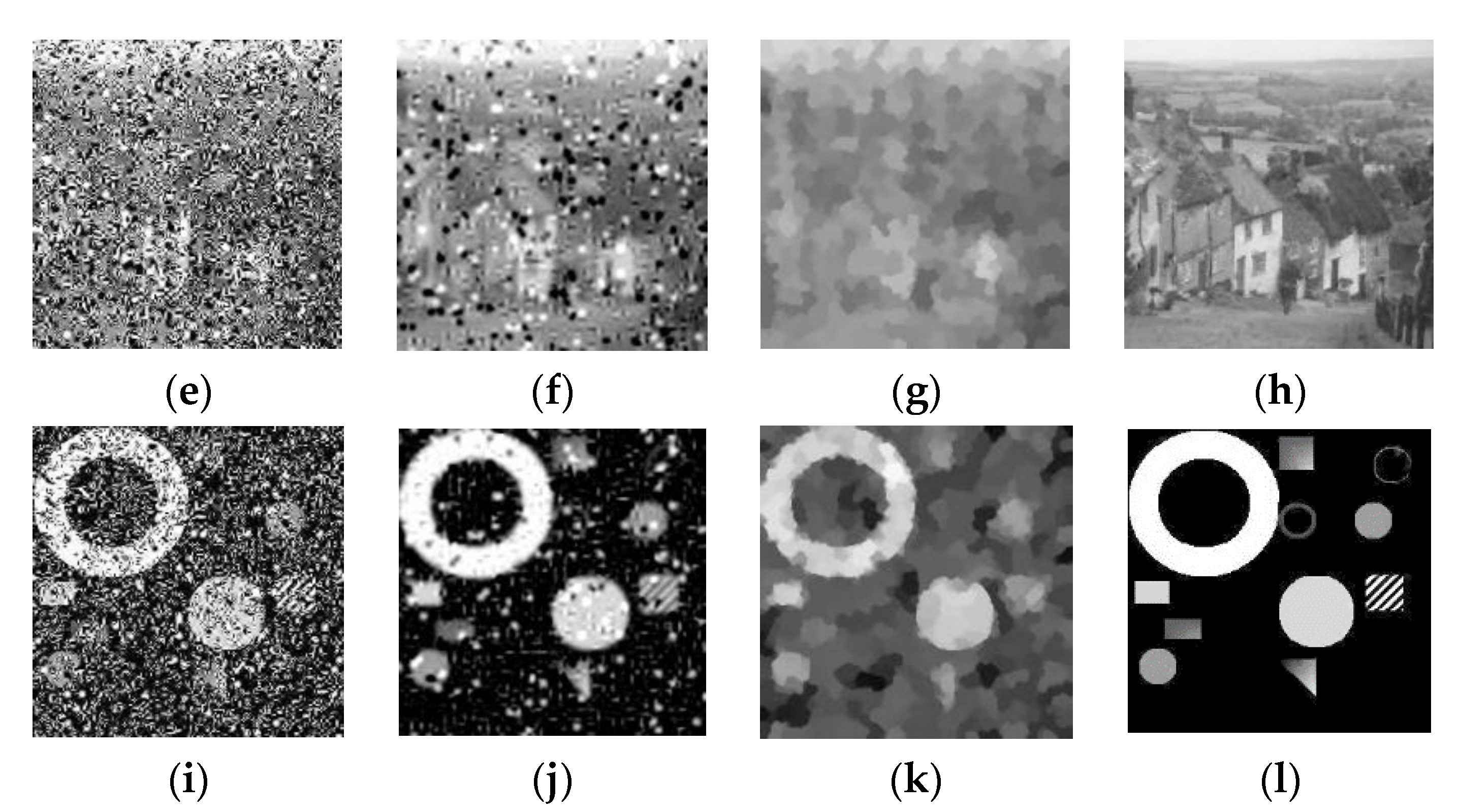
4. Numerical Results

In this section, we give some numerical results to evaluate the performance of three wavelet inpainting models (TVL2, TVL0, TVL1). Three images (shown in Figure 1) are used for test, including “Lenna”, “Goldhill”, and a synthetic image. PSNR is used as a performance evaluation criterion, which is defined by

$$PSNR=10{\log }_{10}\left(\frac{{255}^2}{\Vert u-u^0{\Vert }_2^2}\right)$$

where $u^0$ is the original image, $u$ is the inpainted image.

In this paper, we apply the Daubechies 7-9 biorthogonal wavelets with symmetric extensions at the boundaries for decomposition. In all experiments, we choose ${\nu }_0$ as the acquired wavelet coefficients and $u_0$ as the received image, which is the back projection of ${\nu }_0$. We fix $s=0.125$ (see [27] for details) and $\gamma =1.9\alpha$ (see Proposition 1) for Algorithm 1. In the JPEG 2000 compression standard, the image is decomposed into wavelet sub-bands, and then each sub-band is divided into codeblocks. Therefore, we consider the codeblock loss of the wavelet coefficients in the experiments. For simplicity, we choose the codeblocks of 8 × 8 that randomly spread in the wavelet image as the loss mask. Recently, Wen et al. [22] proposed a primal–dual method for the TVL2 model, which is faster than the method used in [3]. Here, we employ this method to solve the TVL2 model.

The first experiment is to perform the proposed algorithm on the images whose wavelet coefficients are randomly lost but not corrupted by noise. We choose the parameter values as follows: $\lambda =0.1$, $\alpha =1$ for TVL1, $\lambda =0.1$ for TVL2 and $\lambda =4$ for TVL0 [18]; other parameter values for TVL2 and TVL0 are the same as ones in [22] and [18], respectively. We test each of the three images with their partial coefficients lost (10%, 20%, 30%). The PSNR values against the severity of the damage are shown in Figure 2. It is seen that the proposed model is superior to other models in term of PSNR. We show the received and reconstructed Lenna images in Figure 3. From their zoomed in views (Figure 4), we can see that TVL1 model gives better edge reconstruction (see the doorframes).

The second experiment is to perform the proposed algorithm and two other models on the images whose partial wavelet coefficients are randomly lost and corrupted by salt-pepper noise (a typical impulsive noise). For this case, the parameter values were chosen as follows: for TVL1, $\lambda =0.4$, $\alpha =1$; for TVL0 and TVL2, we chose the best $\lambda$ from 1 to 100 with the increment of each step set to 1, while other parameter values for TVL2 and TVL0 were the same as ones in [22] and [18], respectively. Firstly, we randomly corrupted 5% of the acquired wavelet coefficients with salt-pepper noise. The three models were then applied to recovering the images from their partial wavelet coefficients. Figure 5 lists the received images and reconstructed images by the three models from 90% corrupted wavelet coefficients. We can observe that both TVL2 and TVL0 models were not able to recover the damaged coefficients properly, while TVL1 model was able to reconstruct images with sharp edges and clean geometrical shapes. We show the reconstructed images by TVL1 model with 50% wavelet coefficients lost in Figure 6, from which we can see that TVL1 model can still produce images with visually acceptable quality. Secondly, we investigate the robustness of TVL1 model against the salt-pepper noise. In addition to losing 10% coefficients randomly, we corrupt at random 30% of the acquired coefficients with salt-pepper noise. The received and reconstructed images are shown in Figure 7. We can see that TVL1 can restore partial geometrical information, while the received images are severely damaged.

The final experiment is to discuss the parameter $\alpha$, which plays an important role in Algorithm 1. The value of $\alpha$ determines how well the Moreau envelope approximates the function $\mathsf{\Phi }$ in (11). In the following, we experimentally investigated the performance of Algorithm 1 with different $\alpha$. In this experiment, 5% of the acquired wavelet coefficients were randomly corrupted by salt-pepper noise, and 10% of corrupted coefficients were lost. The PSNR value is shown in

Table 1. PSNR values for different $\alpha$.

	α = 1	α = 2	α = 3	α = 5	α = 10
Lenna	23.07	23.07	23.04	22.92	22.59
Goldhill	21.65	21.65	21.64	21.57	21.26
Synthetic	28.54	28.49	28.41	28.20	27.50

. We can see that the solution of the modified model with a smaller $\alpha$ is a better approximate solution of the original model in term of objective metric (PSNR). Meanwhile, we show the plot of PSNR against CPU time for Lenna image in Figure 8. The faster convergence rate is shown with a larger $\alpha$. According to the above two laws, we suggested that the researcher can make a reasonable choice according to the needs of the application.

5. Conclusions

This paper proposed the TVL1 model for inpainting wavelet coefficients corrupted by impulsive noise. The difficulty of numerical treatment lies in the non-differentiability of l¹-norm fitting term. To address this problem, the l¹-norm was smoothed by the corresponding Moreau envelope and then a primal–dual fixed-point algorithm based on proximity operator (PDFP²O) was applied to solving the modified TVL1 model. We considered the existence of solution for the proposed model and the convergence analysis of the developed iterative scheme in this paper. Experiment results show that this method can effectively recover incomplete wavelet coefficients with or without impulsive noise and preserve geometrical information in the pixel domain well.

References

1. Yashtini, M.; Kang, S.H. A fast relaxed normal two split method and an effective weighted TV approach for Euler’s elastica image inpainting. SIAM J. Imaging Sci. 2016, 9, 1552–1581. [Google Scholar] [CrossRef]
2. Ning, W.; Ma, S.; Li, J.; Zhang, Y.; Zhang, L. Multistage attention network for image inpainting. Pattern Recognit. 2020, 106, 107448. [Google Scholar]
3. Chan, T.F.; Shen, J.; Zhou, H.M. Total variation wavelet inpainting. J. Math. Imag. Vis. 2006, 25, 107–125. [Google Scholar] [CrossRef]
4. Ballester, C.; Bertalmio, M.; Caselles, V.; Sapiro, G.; Verdera, J. Filling-in by joint interpolation of vector fields and gray levels. IEEE Trans. Image Process. 2001, 10, 1200–1211. [Google Scholar] [CrossRef] [Green Version]
5. Li, F.; Bao, Z.; Liu, R.H.; Zhang, G.X. Fast image inpainting and colorization by Chambolle’s dual method. J. Vis. Commun. Image R 2011, 22, 529–542. [Google Scholar] [CrossRef]
6. Chan, T.F.; Shen, J. Mathematical models for local non-texture inpaintings. SIAM J. Appl. Math 2002, 62, 1019–1043. [Google Scholar]
7. Cai, J.F.; Chan, R.H.; Shen, Z. A framelet-based image inpainting algorithm. Appl. Comput. Harm. Anal. 2008, 24, 131–149. [Google Scholar] [CrossRef] [Green Version]
8. Chan, R.H.; Chan, T.F.; Shen, L.X.; Shen, Z. Wavelet algorithms for high-resolution image reconstruction. SIAM J. Sci. Comput. 2003, 24, 1408–1432. [Google Scholar] [CrossRef]
9. Huang, Y.; Ng, M.K.; Wen, Y. Fast image restoration methods for impulse and Gaussian noises removal. IEEE Signal Process. Lett. 2009, 16, 457–460. [Google Scholar] [CrossRef]
10. Fuchs, M.; Muller, J. A higher order TV-type variational problem related to the denoising and inpainting of images. Nonlinear Anal. 2017, 154, 122–147. [Google Scholar] [CrossRef] [Green Version]
11. Bertalmio, M.; Sapiro, G.; Caselles, V.; Ballester, C. Image inpainting. In Proceedings of the ACM SIGGRAPH, New Orleans, LA, USA, 23–28 July 2000; pp. 417–424. [Google Scholar]
12. Chan, T.F.; Shen, J. Nontexture inpainting by curvature-driven diffusions. J. Vis. Commun. Image R. 2001, 12, 436–449. [Google Scholar] [CrossRef]
13. Chan, T.F.; Kang, S.H.; Shen, J. Euler’s elastic and curvature-based inpainting. SIAM J. Appl. Math. 2002, 63, 564–592. [Google Scholar]
14. Ren, Z. Adaptive active contour model driven by fractional order fitting energy. Signal Process. 2015, 117, 138–150. [Google Scholar] [CrossRef]
15. Arias, P.; Facciolo, G.; Caselles, V.; Sapiro, G. A variational framework for exemplar-based image inpainting. Int. J. Comput. Vis. 2011, 93, 319–347. [Google Scholar] [CrossRef] [Green Version]
16. Peyré, G.; Bougleux, S.; Cohen, L. Non-local regularization of inverse problems. Inverse Probl. Imaging 2011, 5, 511–530. [Google Scholar] [CrossRef]
17. Jiang, L.; Yin, H. Wavelet inpainting by fractional order total variation. Multidimens. Syst. Signal Process. 2018, 29, 299–320. [Google Scholar] [CrossRef]
18. Yau, A.C.; Tai, X.; Ng, M.K. L0-norm and Total Variation for wavelet inpainting. In Proceedings of the 2nd International Conference on Scale Space & Variational Methods in Computer Vision, Berlin/Heidelberg, Germany, 1–5 June 2009. [Google Scholar]
19. Zhang, H.Y.; Peng, Q.C.; Wu, Y.D. Wavelet inpainting based on p-Laplace operator. Acta Autom. Sin. 2007, 33, 546–549. [Google Scholar] [CrossRef]
20. Chan, R.H.; Yang, J.F.; Yuan, X.M. Alternating direction method for image inpainting in wavelet domains. SIAM J. Imaging Sci. 2011, 4, 807–826. [Google Scholar] [CrossRef]
21. Zhang, X.Q.; Chan, T.F. Wavelet inpainting by Nonlocal total variation. Inverse Probl. Imaging 2010, 4, 191–210. [Google Scholar] [CrossRef]
22. Wen, Y.W.; Chan, R.H.; Yip, A.M. A primal-dual method for total-variation-based wavelet domain inpainting. IEEE Trans. Image Process. 2012, 21, 106–114. [Google Scholar] [CrossRef]
23. Durand, S.; Froment, J. Reconstruction of wavelet coefficients using total variation minimization. SIAM J. Sci. Comput. 2003, 24, 1754–1767. [Google Scholar] [CrossRef] [Green Version]
24. Chan, T.F.; Zhou, H.M. Optimal Constructions of Wavelet Coefficients Using Total Variation Regularization in Image Compression; UCLA CAM Report 00-27; Department of Math. UCLA: Los Angeles, CA, USA, 2000. [Google Scholar]
25. Wu, C.L.; Zhang, J.Y.; Tai, X.C. Augmented Lagrangian method for total variation restoration with non-quadratic fidelity. Inverse Probl. Imaging 2011, 5, 237–261. [Google Scholar] [CrossRef]
26. Goldstein, T.; Osher, S. The Split Bregman method for L1-regularized problems. SIAM J. Imaging Sci. 2009, 2, 323–343. [Google Scholar] [CrossRef]
27. Micchelli, C.A.; Shen, L.X.; Xu, Y.S. Proximity algorithms for image models: Denoising. Inverse Probl. 2011, 27, 045009. [Google Scholar] [CrossRef]
28. Combettes, P.; Wajs, V.R. Signal recovery by proximal forward-backward splitting. Multiscale Model. Simul. 2005, 4, 1168–1200. [Google Scholar] [CrossRef] [Green Version]
29. Chen, P.J.; Huang, J.; Zhang, X. A primal-dual fixed point algorithm for convex separable minimization with applications to image restoration. Inverse Probl. 2013, 29, 025011. [Google Scholar] [CrossRef]
30. Liu, X.; Tang, Y.; Yang, Y. Primal-dual algorithm to solve the constrained second-order total generalized variational model for image denoising. J. Electron. Imaging 2019, 28, 043017. [Google Scholar] [CrossRef]
31. Aujol, J.F.; Gilboa, G.; Chan, T.F.; Osher, S. Structure-texture image decomposition-modeling, algorithms, and parameter selection. Int. J. Comput. Vision. 2006, 67, 111–136. [Google Scholar] [CrossRef]
32. Yang, J.; Yin, W. An efficient TVL1 algorithm for deblurring multichannel images corrupted by impulsive noise. SIAM J. Sci. Comput. 2009, 31, 2842–2865. [Google Scholar] [CrossRef]
33. Chen, F.; Shen, S.; Xu, F.; Zeng, X. The Moreau envelope approach for the L1/TV image denoising model. Inverse Probl. Imaging 2017, 8, 53–77. [Google Scholar] [CrossRef]
34. Rockafellar, R.T.; Wets, R.J. Variational Analysis, 3rd ed.; Springer: New York, NY, USA, 2009; p. 21. [Google Scholar]
Figure 1. Test images. (a) Lenna. (b) Goldhill. (c) Synthetic.
Mathematics 10 02470 g001
Figure 2. PSNR comparison against the severity of damages for three images. (a) Lenna. (b) Goldhill. (c) Synthetic.
Mathematics 10 02470 g002
Figure 3. 10% wavelet coefficients of Lenna are randomly lost. (a) received image. (bd) images reconstructed by TVL2, TVL0, and TVL1, respectively.
Mathematics 10 02470 g003
Figure 4. Zoomed portions of the original and reconstructed Lenna. (a) original image. (bd) images reconstructed by TVL2, TVL0, and TVL1, respectively.
Mathematics 10 02470 g004
Figure 5. 5% wavelet coefficients are corrupted by salt-pepper noise and 10% coefficients are lost. (a,e,i) received images. (b,f,j) images reconstructed by TVL2 with λ = 10. (c,g,k) images reconstructed by TVL0 with λ = 3. (d,h,l) images reconstructed by TVL1.
Mathematics 10 02470 g005aMathematics 10 02470 g005b
Figure 6. 5% wavelet coefficients are corrupted by salt-pepper noise and 50% coefficients are lost. (ac) received images. (df) images reconstructed by TVL1.
Mathematics 10 02470 g006
Figure 7. 30% wavelet coefficients are corrupted by salt-pepper noise and 10% coefficients are lost. (ac) received images. (df) images reconstructed by TVL1.
Mathematics 10 02470 g007
Figure 8. PSNR against CPU time for Lenna image with different α .
Mathematics 10 02470 g008