1. Introduction
Linear mixed models (LMMs) are useful for the statistical analysis of correlated datasets such as longitudinal data. For simplicity, it is usually assumed that both random effects and random errors follow a normal distribution. Under these restrictions, there are several proposals for estimating LMM parameters in the literature; among these, one can refer to Harvill [
1], Fellner [
2], Khuri et al. [
3] and Wu et al. [
4]. For example, Harvill [
1] and Fellner [
2] obtained the maximum likelihood (ML) estimates of parameters in a multifactor normal LMM under heteroscedasticity of random-effect factors. They showed the estimates, in addition to being consistent, were asymptotically normally distributed. However, as pointed out by Zhong and Davidian [
5], using these estimation methods may cause invalid statistical inferences when the data are asymmetric. Therefore, many authors have criticized the common use of the normality assumption (see, e.g., [
6,
7,
8,
9,
10]).
From a practical perspective, the most frequently used method to achieve normality is to apply a transformation on the variables. Although such methods may provide suitable empirical results, they should not be used if a more reasonable theoretical model is available [
11]. Thus, it is of great interest to develop estimation methods in statistical models with flexible distribution assumptions. In this sense, one of the simplest and applicable distributions that provides skewness and contains a normal distribution is the skew-normal distribution introduced by Azzalini [
12]. Although it is old, it is still used in statistical models due to its flexibility and simplicity, especially in complex models where it is difficult to use new generalized skewed distributions. Some new works in this research area are [
13,
14]. In the literature, many authors have studied inferences on parameters in LMMs (with only one random-effect factor) where the random effects or the model random errors follow asymmetric and non-normal distributions (see, e.g., [
5,
7,
8,
9,
15,
16,
17,
18,
19,
20,
21,
22]). Verbeke and Lesaffre [
15], through an extended simulation when the random-effect distribution was misspecified, showed that the standard errors of the parameters needed to be corrected. Arellano-Valle et al. [
18] considered an LMM when both the random-effect factor and the random errors follow the SN distribution. Due to complexity, they derived marginal distributions and implemented an EM algorithm to obtain the ML estimates. They indicated that the estimates had more efficiency than normal estimates when the normality assumption was violated. Lachos et al. [
19] presented an LMM when the random effects followed a multivariate SN independent distribution. They derived the ML estimates of the parameters based on an efficient EM algorithm. They also investigated a technique to predict the response variable. Kheradmandi and Rasekh [
20] followed [
18] and obtained the ML estimates in the LMM when the fixed effects were measured with non-negligible errors. In this work, a multifactor SN–LMM was considered with different variances for the random-effect factors to show how heteroscedasticity, as a freer assumption in random-effect factors, can improve our statistical results. Here, a SN–LMM is an LMM with SN distribution in the model random errors.
A diagnostic analysis is a necessary step in statistical analysis after parameter estimation. The local influence approach, a pioneering work of Cook [
23], is one of the most important diagnostic tools for assessing the stability of the estimation parameters. Due to the complicated calculations of Cook’s local influence approach in statistical models with incomplete data, Zhu and Lee [
24] developed Cook’s approach to these models based on the conditional expectation of a complete-data log likelihood at the E-step of the EM algorithm. To see some applications of Zhu and Lee’s approach, one can refer to [
25,
26,
27,
28]. Local influence analysis for LMMs based on SN distribution had been studied by Bolfarine [
29], Montenegro et al. [
30], and Zeller et al. [
31]. All these works considered local influence diagnostics for an LMM based on SN distribution in the random-effect factor. Furthermore, all perturbation schemes were considered the same. In this work, besides parameter estimation, we developed Zhu and Lee’s local influence diagnostic measures for the LMM under different assumptions on random effects and random errors that were mentioned before. A different perturbation scheme was also considered concerning the previous works. The rest of the paper is structured as follows. In
Section 2, we present the model and obtain distributional facts about the variables that will help us use the EM algorithm. In
Section 3, parameter estimation and random effects prediction are derived via the EM algorithm. In
Section 4, the local influence diagnostic measures for the LMM are extended based on the methodology proposed by Zhu and Lee [
24]. The basic building blocks of three perturbation schemes are also derived. In
Section 5, a simulation study is performed to compare the normal LMM and the SN-LMM, and then a real dataset is analyzed to perform an illustrative comparison. Discussion and conclusions of this paper are given in
Section 6.
2. The Model Definition
Consider the following LMM:
where
is a
vector of parameters, which are fixed effects;
and
are
and
known design matrices, respectively, where
is an
design matrix of the random-effect factor
;
, where
is a
vector of unobservable random effects from
,
;
ε is an
vector of unobservable random errors from
, that is
-dimensional SN distribution with skewness vector
. The variances
are named variance components. We assume that
,
, and
are mutually independent. One may also write
, where
is a block diagonal matrix with the
th block being
, for
, that are called the ratio of variance components.
The above assumptions conclude that
and so the joint distribution of the vectors
and
is obtained as follows:
where
stands for the
-variate normal density function with mean
and covariance matrix
and
represents the cumulative distribution function of
.
From (2), the marginal density of
would be as follows:
where
,
so that
is a symmetric, non-singular matrix;
; and where
. Therefore,
has a generalized SN distribution.
Based on the distribution of
, the log-likelihood function of
is given by
where
.
As can be seen, there is no obvious solution for the direct maximization of Equation (3), and the likelihood function has to be maximized numerically. Using numerical approaches, besides the high computational costs and lack of robustness to the starting values, causes some problems for the maximization due to the term
. Therefore, corresponding to previous studies in the field of using the skew family in modeling (see, e.g., [
8,
9,
18,
19,
20,
22,
27]), an EM algorithm was applied to reduce computation complexity with high efficiency.
The EM algorithm, introduced by Dempster et al. [
32], is a famous iterative algorithm for ML estimation in incomplete data models. One of the major reasons for its popularity is the M-step that includes maximization of a likelihood function based on complete data, which is often computationally simple. It is also not very sensitive to the starting parameter values.
Let
represent the truncated normal distribution with parameters
and
and truncation range
. If the distribution of
is written as
the joint distribution of
and the missing variable
will be
Based on the above joint distribution, the conditional distribution of
is obtained as
Hence,
. Now, with the help of the properties of the truncated normal distribution [
33], we have
and
To predict the random effects, we first need the conditional distribution of
given by
where
Now, the conditional log-likelihood function of
––given
,
and
––is obtained as
As seen again, like has the term and so, to predict , based on the ML method, we use the EM algorithm.
To do this, we first rewrote the conditional distribution of
as
So, the conditional distribution of
and the missing variable
given
is equal to
The above equation concludes that the conditional distribution of the missing variable
given
and
is equal to
As seen,
and hence,
and
3. Parameter Estimation via the EM Algorithm
Now, let
be a vector of observed responses and
be a missing observation. Then, the complete log-likelihood function associated with
will be obtained as
where
does not depend on unknown parameters.
If
is the estimate in the
th iteration, then the expected complete log-likelihood function would be
where
and
are calculated by substituting
in Equations (4) and (5), respectively.
To obtain a new estimate
, the M-step maximizes
with respect to
. This was obtained as a solution of the following equations:
and
If we define
, then from the Equation (9), the estimation of
, is given by
Before the estimation of variance components, we presented a realized value of the random effects. In a similar way for fixed effects (See
Appendix A.1 for more details.), the ML prediction of
was given by
where
and
were calculated by substituting
and
into Equations (7) and (8), respectively.
Then, for the
th random-effect factor, we have
From Equation (9), the estimates of variance components were derived as
and
where
is
th diagonal block of the matrix
(See
Appendix A.2 for more details.). By substituting
and
with
and
, respectively, in the above equation, one can obtain another estimator for
based on
similar to its corresponding estimator in the normal LMM. This estimator would be as follows:
where
.
Finally, the ML estimates of skewness parameters would be
where
is
evaluated at updated
,
and
.
The above algorithm stops when a reasonable convergence rule is satisfied (e.g., ). A set of adequate starting values can be obtained by solving the normal LMM for , and , and the sample skewness coefficient of the residuals or zero values for . But, as recommended in the literature, the EM algorithm should be run several times with different starting values.
4. Local Influence Analysis
Cook’s local influence method was used to evaluate the influence of various minor model perturbations on the parameter estimates. Inspired by the general idea of the EM algorithm, Zhu and Lee [
24] generalized the local influence diagnostic method to general statistical models with incomplete data based on a Q-function. Here, we briefly studied a natural extension of this procedure to SN–LMM. In this section, we assumed that the
’s were known. If the
’s were unknown, the ML estimates would have been placed back into
, so the vector
would have been
.
If we let
be a n-dimensional vector of perturbations varying in open region
, the perturbed complete-data log-likelihood function would be denoted by
. It is assumed that there exists
, a vector of no perturbation, such that
for all
. Let
be the maximum value of the
, where
denotes the ML estimate under
. To evaluate the influence of minor perturbations on the ML estimate
, one may regard the Q-displacement function, defined as follows:
Zhu and Lee [
24] suggested studying the local behavior of
around
. Corresponding to their proposal, the normal curvature in the direction of some unit vector
, given by
, can be employed to summarize the local behavior of the Q-displacement function, where
in which
and
Since most influence measures proposed in the statistical literature are closely related to a spectral decomposition of , we used this expression to detect influential observations. Let be the spectral decomposition of where are the eigenvalue–eigenvector pairs of the matrix with , and is the associated orthonormal basis.
Following Zhu and Lee [
24] and Lu and Song [
34], the assessment of influential observations was based on
where
. The influence measure
may be obtained through
where
is an
vector with the
ith element equal to one and all other elements equal to zero. Moreover, corresponding to Lee and Xu [
35], we used the cut-off point
to consider the
ith observation as influential, where
is a constant, chosen according to the real application, and
denotes the standard deviation of
.
4.1. The Hessian Matrix
To achieve the local influence diagnostic measures for a particular perturbation scheme, we needed to compute
. It follows from (9) that the Hessian matrix has elements given by
4.2. Perturbation Schemes
In this section, we present three distinct perturbation schemes for the model defined in (1).
4.2.1. Perturbation of the Response Variable
A perturbation of the response variable
is defined as
, where
is the standard deviation of
. In this case,
and
From (10), the matrix
has the following elements.
4.2.2. Perturbation of the kth Column of the Matrix
We considered altering the
kth column matrix
, i.e.,
, by taking
where
is the standard deviation of
and
represents no perturbation. In this case, the perturbed
-function took the form
where
. It follows from (11), that the elements of the matrix
were given by
4.2.3. Perturbation of the Dispersion Matrix of the Errors
We modified the dispersion matrix of errors, i.e.,
, to
where
is a diagonal matrix with diagonal elements
. The point representing no perturbation is
. In this case, the perturbed
-function was obtained as
where
,
, and
. From (12), we obtained the elements of
.
The
kth column of the matrix
was given by
where
is the
kth column of matrix
. Also, the
kth element of the vector
was obtained by
Finally, the
kth column of the matrix
was achieved by
where
and
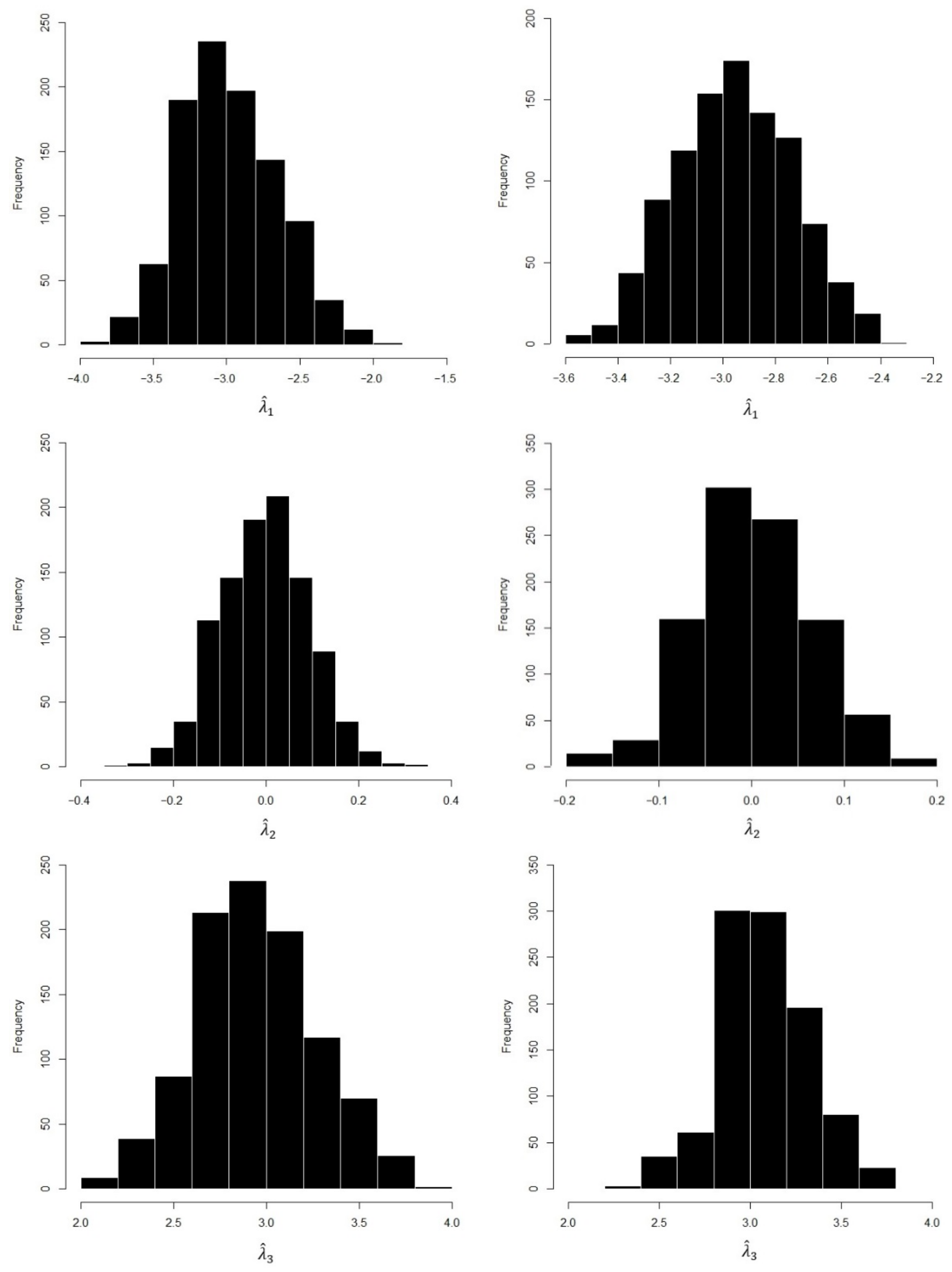
6. Conclusions
The study of a multifactor normal LMM under heteroscedasticity was done by authors such as [
1,
2]. They showed that the ML method for estimation of the parameters performed well and the estimates had good properties such as consistency and asymptotic normal distribution. When the normality test of model errors or random effects was rejected, the derived estimates did not lead to satisfactory results. Therefore, LMMs (only with a random-effect factor) based on skewed distributions were presented by several authors. When the normality assumption did not hold for the model errors or the random-effect factor, these models performed well in comparison to those under the normality assumption. Additionally, diagnostic analyses showed these models decreased the effect of outliers. Recent research showed that new generalized skewed distributions usually have a better fit than simpler skewed distributions (see e.g., [
38,
39]). Clearly, using these distributions in LMMs can be also considered (see e.g., [
40]), but, as mentioned before, the complexity of calculations in complicated models makes a case for using the simple but flexible SN distribution (See using SN distribution in some new complicated models [
13,
14]). Therefore, we considered SN distribution for the model errors in the multifactor LMM under heteroscedasticity in random-effect factors. Our main goals involved parameter estimation and the local influence method for the multifactor SN–LMM under heteroscedasticity in random-effect factors. At first, we expanded an EM-based algorithm, as many in the literature proposed, to estimate the model parameters. We also obtained a closed form to estimate variance components using this method. Then, we applied Zhu and Lee’s approach to extend the local influence method to this model. Empirical studies, a simulation study and a real data example, were carried out to see the behavior of our estimators. Our findings followed previous results in this field. The simulation results––consistency, low dispersion, and asymptotic normal distribution––showed that the estimators performed well, even for finite sample sizes. It was also observed that ignorance of skewness when the error model followed from a skewed distribution like SN made unsuitable outcomes. Finally, through a real example, it was shown that taking into account both heteroscedasticity in random-effect factors and election a skewed distribution for random errors in the fitted model improved statistical results in comparison to other works that considered at most one of them. Additionally, in this case, we observed the robustness of the ML estimators through the local influence method. Finally, any skewed distributions contained symmetrical distributions in special cases. When the assumption of symmetry held for random variables in a sensitivity analysis of any model, skewed distributions were not recommended due to additional parameter costs. Extending this work when both random-effect factors and model errors have SN distribution is theoretically and computationally hard, but that will be our goal in a subsequent work. Moreover, generalized skewed distributions for the model errors or the random-effect factors in the multifactor LMM, along with diagnostic measures, are proposed for future work.


 ,
, 


