
Mathematical Model of Hepatitis B Virus Treatment with Support of Immune System


Abstract
:1. Introduction
2. Introduction of the Model
3. Classification of Equilibrium Points
4. Influence of Right-Hand Side Changes on Solution Behavior
5. Exponential Stability of the System with Delays in Upper and Lower Limits of Control Function
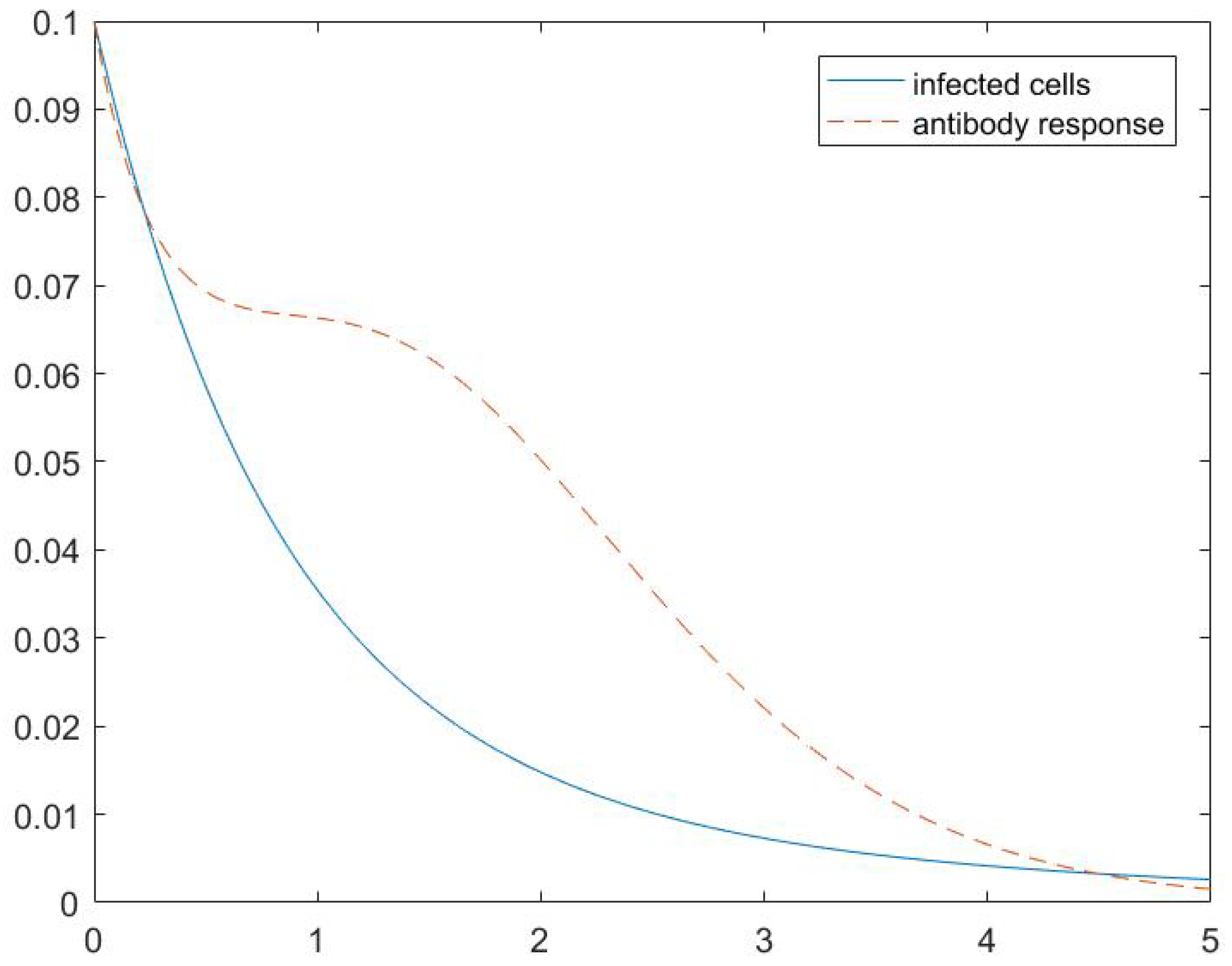
6. Simulations
7. Conclusions
Funding
Institutional Review Board Statement
Informed Consent Statement
Data Availability Statement
Conflicts of Interest
References
- Tang, L.S.Y.; Covert, E.; Wilson, E.; Kottilil, S. Chronic Hepatitis B Infection: A Review. J. Am. Med. Assoc. 2018, 319, 1802–1813. [Google Scholar] [CrossRef] [PubMed]
- Long, C.; Qi, H.; Huang, S.H. Mathematical modeling of cytotoxic lymphocyte-mediated immune response to hepatitis B virus infection. J. Biomed. Biotechnol. 2008, 2008, 743690. [Google Scholar] [CrossRef] [PubMed] [Green Version]
- Poh, Z.; Goh, B.B.; Chang, P.E.; Tan, C.K. Rates of cirrhosis and hepatocellular carcinoma in chronic hepatitis B and the role of surveillance: A 10-year follow-up of 673 patients. Eur. J. Gastroenterol. Hepatol. 2015, 27, 638–643. [Google Scholar] [CrossRef] [PubMed] [Green Version]
- Parkin, D.M. The global health burden of infection-associated cancers in the year 2002. Int. J. Cancer 2006, 118, 3030–3044. [Google Scholar] [CrossRef] [PubMed] [Green Version]
- European Association for the Study of the Liver. EASL 2017 Clinical Practice Guidelines on the management of hepatitis B virus infection. J. Hepatol. 2017, 67, 370–398. [Google Scholar] [CrossRef] [PubMed] [Green Version]
- Colombatto, P.; Civitano, L.; Bizzarri, R.; Oliveri, F.; Choudhury, S.; Gieschke, R.; Bonino, F.; Brunetto, M.R.; Peginterferon Alfa-2a HBeAg-Negative Chronic Hepatitis B Study Group. A multiphase model of the dynamics of HBV infection in HBeAg-negative patients during pegylated interferon-α, lamivudine and combination therapy. Antivir. Ther. 2006, 11, 197–212. [Google Scholar] [CrossRef] [PubMed]
- Nowak, M.A.; Bonhoeffer, S.; Hill, A.M.; Boehme, R.; Thomas, H.C.; McDade, H. Viral dynamics in hepatitis B virus infection. Proc. Natl. Acad. Sci. USA 1996, 93, 4398–4402. [Google Scholar] [CrossRef] [PubMed] [Green Version]
- Perelson, A.S.; Ribeiro, R.M. Hepatitis B virus kinetics and mathematical modeling. Semin. Liver Dis. 2004, 24, 11–16. [Google Scholar] [CrossRef] [PubMed]
- Wain-Hobson, S. Virus Dynamics: Mathematical Principles of Immunology and Virology. Nat. Med. 2001, 7, 525–526. [Google Scholar] [CrossRef]
- Yousdi, N.; Hattaf, K.; Rachik, M. Analysis of a HCV model with CTL and antibody responses. Appl. Math. Sci. 2009, 3, 2835–2845. [Google Scholar]
- Domoshnitsky, A.; Volinsky, I.; Pinhasov, O. Some developments in the model of testosterone regulation. AIP Conf. Proc. 2019, 2159, 030010. [Google Scholar] [CrossRef]
- Volinsky, I.; Bunimovich-Mendrazitsky, S. Mathematical analysis of tumor-free equilibrium in BCG treatment with effective IL-2 infusion for bladder cancer model. AIMS Math. 2022, 7, 16388–16406. [Google Scholar] [CrossRef]
- Domoshnitsky, A.; Volinsky, I.; Pinhasov, O.; Bershadsky, M. Stability of functional differential systems applied to the model of testosterone regulation. Bound. Value Probl. 2019, 1, 184. [Google Scholar] [CrossRef]
- Volinsky, I.; Lombardo, S.D.; Cheredman, P. Stability Analysis and Cauchy Matrix of a Mathematical Model of Hepatitis B Virus with Control on Immune System near Neighborhood of Equilibrium Free Point. Symmetry 2021, 13, 166. [Google Scholar] [CrossRef]
- Milner, P.B.; Wang, J. Acute Hepatitis B Viral Infection in a Patient with Common Variable Immunodeficiency: A Case Report. Am. J. Gastroenterol. 2018, 113, S1362. [Google Scholar] [CrossRef]
- Li, T.Y.; Yang, Y.; Zhou, G.; Tu, Z.K. Immune suppression in chronic hepatitis B infection associated liver disease: A review. World J. Gastroenterol. 2019, 25, 3527. [Google Scholar] [CrossRef] [PubMed]
- Paroli, M.; Accapezzato, D.; Francavilla, V.; Insalaco, A.; Plebani, A.; Balsano, F.; Barnaba, V. Long-lasting memory-resting and memory-effector CD4+ T cells in human X-linked agammaglobulinemia. Blood J. Am. Soc. Hematol. 2002, 99, 2131–2137. [Google Scholar] [CrossRef] [PubMed] [Green Version]
- Lincoln, D.; Petoumenos, K.; Dore, G.J.; Australian HIV Observational Database. HIV/HBV and HIV/HCV coinfection, and outcomes following highly active antiretroviral therapy. HIV Med. 2003, 4, 241–249. [Google Scholar] [CrossRef] [PubMed] [Green Version]
- Agarwal, R.P.; Berezansky, L.; Braverman, E.; Domoshnitsky, A. Nonoscillation Theory of Functional Differential Equations with Applications; Springer: New York, NY, USA, 2012. [Google Scholar]
- Chenar, F.F.; Kyrychko, Y.N.; Blyuss, K.B. Mathematical model of immune response to hepatitis B. J. Theor. Biol. 2018, 447, 98–110. [Google Scholar] [CrossRef] [PubMed] [Green Version]


Publisher’s Note: MDPI stays neutral with regard to jurisdictional claims in published maps and institutional affiliations. |
© 2022 by the author. Licensee MDPI, Basel, Switzerland. This article is an open access article distributed under the terms and conditions of the Creative Commons Attribution (CC BY) license (https://creativecommons.org/licenses/by/4.0/).
Share and Cite
Volinsky, I. Mathematical Model of Hepatitis B Virus Treatment with Support of Immune System. Mathematics 2022, 10, 2821. https://doi.org/10.3390/math10152821
Volinsky I. Mathematical Model of Hepatitis B Virus Treatment with Support of Immune System. Mathematics. 2022; 10(15):2821. https://doi.org/10.3390/math10152821
Chicago/Turabian StyleVolinsky, Irina. 2022. "Mathematical Model of Hepatitis B Virus Treatment with Support of Immune System" Mathematics 10, no. 15: 2821. https://doi.org/10.3390/math10152821
APA StyleVolinsky, I. (2022). Mathematical Model of Hepatitis B Virus Treatment with Support of Immune System. Mathematics, 10(15), 2821. https://doi.org/10.3390/math10152821