The Development of PSO-ANN and BOA-ANN Models for Predicting Matric Suction in Expansive Clay Soil

Abstract

Disasters have different shapes, and one of them is sudden landslides, which can put the safety of highway users at risk and result in crucial economic damage. Along with the risk of human losses, each day a highway malfunctions causes high expenses to citizens, and repairing a failed highway is a time- and cost-consuming process. Therefore, correct highway functioning can be categorized as a high-priority reliability factor for cities. By detecting the failure factors of highway embankment slopes, monitoring them in real-time, and predicting them, managers can make preventive, preservative, and corrective operations that would lead to continuing the function of intracity and intercity highways. Expansive clay soil causes many infrastructure problems throughout the United States, and much of Mississippi’s highway embankments and fill slopes are constructed of this clay soil, also known as High-Volume Change Clay Soil (HVCCS). Landslides on highway embankments are caused by recurrent volume changes due to seasonal moisture variations (wet-dry cycles), and the moisture content of the HVCCS impacts soil shear strength in a vadose zone. Soil Matric Suction (SMS) is another indication of soil shear strength, an essential element to consider. Machine learning develops high-accuracy models for predicting the SMS. The current work aims to develop hybrid intelligent models for predicting the SMS of HVCCS (known as Yazoo clay) based on field instrumentation data. To achieve this goal, six Highway Slopes (HWS) in Jackson Metroplex, Mississippi, were extensively instrumented to track changes over time, and the field data was analyzed and generated to be used in the proposed models. The Artificial Neural Network (ANN) with a Bayesian Regularization Backpropagation (BR-BP) training algorithm was used, and two intelligent systems, Particle Swarm Optimization (PSO) and Butterfly Optimization Algorithm (BOA) were developed to optimize the ANN-BR algorithm for predicting the HWS’ SMS by utilizing 13,690 data points for each variable. Several performance indices, such as coefficient of determination (R²), Mean Square Error (MSE), Variance Account For (VAF), and Regression Error Characteristic (REC), were also computed to analyze the models’ accuracy in prediction outcomes. Based on the analysis results, the PSO-ANN outperformed the BOA-ANN, and both had far better performance than ANN-BR. Moreover, the rainfall had the highest impact on SMS among all other variables and it should be carefully monitored for landslide prediction HWS. The proposed hybrid models can be used for SMS prediction for similar slopes.

1. Introduction

Because of acceptable engineering fill materials’ limitations, much of Mississippi’s highway embankments and fill slopes are constructed of High-Volume Change Clay Soil (HVCCS). In addition to causing many infrastructural problems throughout the United States, this highly plastic clay soil is also a contributing factor to problems in the Jackson Metropolitan Area. Because of its high shrink- swell potential (expansive clay soil such as Yazoo clay), HVCCS exhibits swelling and shrinkage behavior when exposed to changes in Volumetric Soil Moisture Content (VSMC). The HVCCS experiences volume changes due to wetting and drying cycles and seasonal moisture variations [1,2]. Landslides on highway embankments are caused by recurrent volume changes in the presence of rainfall, resulting in substantial repair and reconstruction costs (Figure 1). The highway cut and fill slopes were constructed at a steeper angle in several areas throughout Mississippi, particularly in the vicinity of the metropolitan Jackson area [3].

Furthermore, Yazoo clay is used to construct many of these Highway Slopes (HWS). Previous studies have revealed that the increase in pore water pressure and decrease in soil strength caused by progressive wetting of near-surface soil during rainfall would lead to failure [3,4,5]. In other words, the change in VSMC in the soil layers relates to the amount of rainwater infiltration that occurs because of total rainfall frequencies. The VSMC of the Yazoo clay, which has a high-volume change, impacts the shear strength of soil in a vadose zone [6]. Having negative impacts of excessive VSMC in Yazoo clay, recurrent shallow landslides is one of the growing concerns in Mississippi in recent years. Understanding the behavior of Yazoo clay in terms of Soil Matric Suction (SMS) is critical for improving the design standards, reducing the detrimental effect of the volume change behavior of the expansive clay, and mitigating such problems.

The impact of rainfall risks such as high rainfall intensity and low permeability for use in flood management [7], rainfall-induced landslide susceptibility [8,9], Post-wildfire extreme rainfall events [10], and stormwater runoff [11,12] were discussed in previous works. Rainfall-induced slope failure is a common problem in areas with slopes constructed on high plasticity clay soil. Usually, soils have high matric suction with low VSMC at the vadose zone, resulting in a high safety factor for the slope. However, water infiltrates through the slope during the rainfall, which saturates the slope and may reduce the matric suction. As a result, the slope may become unstable and lead to failure. Most of these failures involve shallow surface slides with depths of less than 3 m (10 ft.) and they require periodic maintenance [3,13].

HWS is an integral part of the efficient movement of the U.S. nation’s Transportation Infrastructure System (TIS), which includes approximately 4 million miles of public highways and roads [14,15]. The traffic volume has increased by 17% over the past decade. HWS are exposed to environmental, climatic, and traffic conditions. Over time, these contributing factors can impact HWS stability. These factors contribute to causing slope failures that are hazardous to highway structures and the traveling public. Moreover, numerous principal components are involved in the HWS as part of TIS, such as efficiency, sustainability, resiliency, the impact of extreme events, and construction. Each is an important part of keeping soil working well for slope stability. The HSSR is one of the most critical factors in the TIS. It is required to preserve progressive, predictive, and permanent actions as well as undertake precautious activities based on recorded real-time field monitoring data to improve the HSSR and to minimize highway failures (with slope stability focus). Establishing and implementing the required infrastructure for attaining the field data is essential. The data classifications are believed to lead to intelligent health monitoring-based predictive models.

Highways are vital for city connectivity, and landslides interacting with populated regions and transportation infrastructure may cause human and economic losses. Because road networks are essential to a society’s economic and social growth, maintaining user safety is a top priority for decision-makers and stakeholders [16]. Based on this study, as part of proactive activities toward the path of sustainability and resiliency, we can monitor the performance of the slopes and take the necessary and prompt actions by implementing a couple of sensors at the HWS and detecting early signs of movement. In the proposed study, the SMS of the slope soil body was predicted by real-time field monitoring data. The SMS is another indication of the soil shear strength, which inspectors can investigate for the preliminary assessment of the slope stability analysis. In addition, using available local and historical Soil Water Retention Curve (SWRC) and predicted SMS, inspectors can estimate the VSMC, which is another effective soil stability parameter. You may imagine how many operations (including but not limited to traffic, construction, time, expense, accessibility, etc.) would need to be planned, coordinated, executed, and completed for a single HWS failure on any state or interstate road. Therefore, the proposed study has the potential to be implemented and save a great deal of time and cost (asset management).

In unsaturated situations, an accurate SMS prediction is critical for determining the level of soil stress by which the HWS’ landslide risks can be managed and prevented. Due to the rainfall and climatic variation in Mississippi, slope failures are common in highway embankments constructed by HVCCS. It is believed that a predictive time series analysis is necessary to determine the interaction between rainfall, SMS, air temperature, VSMC, and soil temperature in terms of seasonal and temporal variations. Seasonal distribution is affected by rainfall volume, while temporal distribution is affected by temperature, which both affect the variation of SMS at different depths. The primary objective of the current study is to develop an accurate data-driven model for predicting SMS containing an Artificial Neural Network (ANN), with a Bayesian Regularization Back-Propagation (BR-BP) training-based algorithm (ANN-BR), PSO-ANN (Particle Swarm Optimization), and BOA-ANN (Butterfly Oprimization Algorithm) models, hybrid intelligent systems, as approaches for SMS prediction for expansive clay that incorporates a large dataset of field instrumentation observations. The term “hybrid” is used in this article to demonstrate technically utilizing PSO or BOA with the conventional ANN. These hybrid intelligent developed models not only help to understand the mechanism behind actual in situ SMS variations over time but could also be used as a point of reference for early symptoms of soil body movements.

2. Background

2.1. ANN

ANN is an efficient approach to self-learning. Human learning is evoked by using a biologically inspired data processing system that can convert internal network analysis into a beneficial output during training. Indeed, ANNs are a type of relatively classical artificial intelligence algorithm that has been effectively applied in a wide variety of fields. However, ANNs may not perform well in time series prediction. It has recently been recognized as a viable strategy for implementation in various areas. Networks may modify the assigned neurons in hidden layers when the output is insufficient. The input variables of the ANN algorithm feed hidden layers of transfer functions. Linear, log sigmoid, and tan sigmoid are some examples of transfer functions. Neurons will use any differentiable transfer function in this state. Additionally, ANNs assess data via the use of feed-forward and feedback classifiers. ANNs can accurately analyze pattern recognition, and non-linear multiplex issues. Functional networks have input, transfer function, and output correlation [17].

2.2. Levenberg-Marquardt Training Algorithm

The Levenberg-Marquardt (LM) ANN approach is comparable to the Gauss-Newton method (GNM). GNM is a quick nonlinear trend classification and optimization technique. Convergence occurs more quickly when there are fewer neurons [18]. Due to the iterative nature of the GNM, it may reveal low function boundaries. The GNM may then iteratively find unknowns in this manner. That is, it solves nonlinear problems optimally. The parameter correlation is calculated using the least-squares fit to a data collection. Using nonlinear least squares, unknown nonlinear variables are annotated.

2.3. BR-BP Training Algorithm

Prior to optimizing the BR training method for selecting the optimal network hyperparameters and training choices, it is necessary to establish the neural network architecture and training alternatives. Optimizing the BR training algorithm is an effective method for optimizing hyperparameters in classification and regression models. The Bayesian Regularization Back Propagation Training Technique (Trainbr) is a back propagation training algorithm that iteratively updates the Bayesian Regularization optimization algorithm using weight and bias variables. It then determines the optimal combination of these parameters to create a robust network to generalization errors and noise. Nie et al. (2019) proposed a Bayesian network-based prediction model for rainfall-induced slope stability [19]. The ultimate objective of many academics is to create the Bayesian network method for reliable prediction models [20,21].

2.4. Hybrid Intelligent Models

Soft computing and artificial intelligence techniques have been effectively emphasized in numerous science and engineering fields, particularly civil and geotechnical engineering [22,23,24,25]. Ann-based models have a wide variety of use in the prediction and forecasting of disasters by using time series data. Some previous articles considered a large-scale framework for daily hydrometeorological flow forecasting models in Canada [26], landslide risk assessment with PSO-ANN, grey wolf optimized based artificial neural network (GW-ANN), grey wolf optimized based random forest (GW-RF) [9], and river flood prediction using fuzzy neural networks [27]. The ANN approach has been successfully used to generate computational algorithms for various geophysical applications, including soil characteristics, weather and climate forecasting, remote sensing, and so on [28,29]. Predictive SMS models could be applied and employed in a wide range of sectors, including geotechnical engineering, agriculture, meteorology, and hydrology. Also, hybrid models could be used in transportation geotechnics to ensure the system is safe and better manage its conditions during extreme and unpredictable climatological events. A PSO can be considered one of the best candidates to optimize the ANN in geotechnical fields and specifically for predicting clay matrices [30,31]. Furthermore, when used as part of the asset management implementation process, the ANN-based model can considerably reduce the issues associated with the repair, maintenance, and renewal programs in the event of future extreme events. The use of predictive models will make some fundamental concerns clearer, particularly in geotechnical engineering applications. For example, knowing what SMS variations are likely to occur will contribute to the design of climate-adaptive transportation infrastructure, saving money and time.

Indirect assessment of SMS in expansive soils using a back-propagation ANN has been scarecly emphasized in the literature. However, the ANN-based approach has certain limitations, such as being locked in local minima and exhibiting a slow learning rate. Combining ANNs with metaheuristic optimization methods such as PSO and BOA can help to overcome these constraints. It has been demonstrated that employing the PSO algorithm improves the performance and the generalization of ANNs when applied to geotechnical engineering challenges [32,33].

The indirect application of this study is a way to prevent landslides and HWS failures. The direct application is creating a predictive model for the unsaturated properties of clay soil. Although the literature has few studies on implementing the aforementioned hybrid models (PSO-ANN and BOA-ANN) for clay soil matric suction prediction models, there are numerous studies on indirect applications, such as those listed in the following. The PSO-ANN technique has been applied for the prediction of Landslide Susceptibility Mapping (LSM) [30,34,35], landslide susceptibility assessment [36,37], the prediction of slope factor of safety [38], earthquake-induced landslide assessment [39], a risk assessment of rainfall-induced landslides [9], and predicting landslide displacement using the interval estimation method [40] in recent years. Zhang et al. (2021) utilized various intelligence algorithms such as PSO, GA, and new swarm intelligence to select the characteristic wavelengths of VSMC [41]. It should be emphasized that the use of the BOA-ANN for predicting soil index and mechanical properties, as well as other geotechnical-related events, is limited. Lohar et al. (2021) utilized and compared different methods as well as BOA-ANN for slope stability analysis through optimizing different geotechnical parameters [42].

3. Methodology

The aims of this section were accomplished in two main steps: the data analysis and developing the predictive model. Section 3.1 comprises the field instrumentation program, data extraction, and data validation. Finally, predictive model development was conducted by utilizing machine learning techniques for targeting the SMS values.

3.1. Data Analysis

3.1.1. Field Instrumentation Program

Six HWS were explored in the Jackson metropolitan area, Mississippi, which is constructed on Yazoo clay (Figure 2). The slopes varied from 2 H:1 V to 6 H:1 V, and the surface was covered with naturally growing grass. Extensive field equipment was installed on each of the six slopes to measure SMS, soil temperature, air temperature, and rainfall. The sensors were positioned at the crest, middle, and toe of the six HWS. Moisture and water potential sensors were installed at 1.5 m, 3 m, and 4.5 m depths in each of the six HWS (Figure 2).

3.1.2. Data Extraction

Levels of 1.5 m, 3 m, and 4.5 m depths for an 18-month from September 2018 to March 2020 monitoring interval in six HWS at Jackson Metropolitan, Mississippi, were used for the research investigation. Moreover, the rain gauge, data recorder, and connector for the moisture sensor were located toward the top of the slope for continuous monitoring for each site. The 1.5 m, 3 m, and 4.5 m depth sensors were programmed with hourly data. Air temperature, soil temperature, rainfall, VSMC, and SMS data were gathered every two weeks for data processing. Therefore, for the above time frame, 13,690 hourly data were received from each sensor mentioned in Figure 3. Hence, 13,690 related data points were created as separate time-series datasets for each input and one output variable. The layout, the installing levels of sensors that were repeated for each six HWS, and the sensors’ models are shown in Figure 3. Because this research considered six HWS, sensors were installed on the top (1.5 m), middle (3 m), and toe (4.5 m) of each HWS; in total, 18 data sets were made; and each one had 13,690 hourly time series data.

Based on the data from the field instrumentation, variations of in situ SMS and VSMC at 1.5 m, 3 m, and 5 m depths with rainfall are presented in Figure 4, Figure A1 and Figure A2. The sensors collect data at the slope’s crest, middle, and toe. Because of the high amount of precipitation, seasonal changes, and other factors (cracks, high vertical permeability, the presence of perched water zones, fully saturated condition, soil body movement near the instrumentation, etc.), SMS and VSMC changed at different depths for all six HWS. The VSMC and SMS are the unsaturated soil properties and are two different parameters. In simple terminology, the soil matric suction is equivalent to the soil shear strength and will vary for different soil types. The soil stratigraphy for all reference HWS is high plastic expansive clay soil. It is observed that the slope has shown variations of both SMS and VSMC values at all three depths for all six HWS. However, the matric suction has shown less variation. The constant low value at the matric suction signifies that the soil is practically close to a fully saturated condition. This is likely possible when perched water conditions are formed on the slope. The high variation of the VSMC indicated the infiltration of the rainwater into these surface cracks. It is unlikely that a perched water table exists on this slope and was not the reason for the observed moisture variations. The constant VSMC on the slope is highly possible if no moisture variation has taken place or the soil is in a fully saturated condition.

As demonstrated in

Table 1. Preliminary detailed statistics for the constructed dataset for HWS 1.

Depths	VSMC	Air Temperature (°C)	Rainfall (mm)	Soil Temperature (°C)	Suction (kPa)
1.5 m Depth
Max	0.55	45.361	48.00	25	12.698
Min	0.426	−7.082	0.00	15.829	9.227
Average	0.520	18.218	0.208	20.483	10.372
Median	0.523	18.528	0.00	20	10.101
Standard deviation	0.019	10.106	1.574	2.914	0.654
3 m Depth
Max	0.54	45.361	48.00	24.766	17.90
Min	0.490	−7.082	0.00	17.433	9.206
Average	0.518	18.218	0.208	20.830	10.277
Median	0.516	18.528	0.00	20.566	9.718
Standard deviation	0.005	10.106	1.574	2.480	1.509
4.5 m Depth
Max	0.50	45.361	48.00	22.566	11.178
Min	0.377	−7.082	0.00	19.366	9.983
Average	0.453	18.218	0.208	21.101	10.236
Median	0.457	18.528	0.00	21.233	10.167
Standard deviation	0.017	10.106	1.574	1.043	0.243

,

Table A1. Preliminary detailed statistics for the constructed dataset HWS 2.

Depths	VSMC	Air Temperature (°C)	Rainfall (mm)	Soil Temperature (°C)	Suction (kPa)
1.5 m Depth
Max	0.47	51.929	48.00	27.666	267.874
Min	0.343	−4.366	0.00	8.367	8.767
Average	0.409	19.116	0.211	19.744	22.687
Median	0.407	18.835	0.00	18.166	9.599
Standard deviation	0.027	10.532	1.484	5.124	46.336
3 m Depth
Max	0.62	51.929	48.00	25.562	24.067
Min	0.445	−4.366	0.00	11.565	9.600
Average	0.521	19.116	0.211	20.725	10.716
Median	0.534	18.835	0.00	20.4	10.433
Standard deviation	0.036	10.532	1.484	3.30	1.776
4.5 m Depth
Max	0.48	51.929	48.00	31.109	12.869
Min	0.445	−4.366	0.00	19.633	9.599
Average	0.456	19.116	0.211	22.101	10.065
Median	0.450	18.835	0.00	22.45	10.010
Standard deviation	0.010	10.532	1.484	1.476	0.329

,

Table A2. Preliminary detailed statistics for the constructed dataset HWS 3.

Depths	VSMC	Air Temperature (°C)	Rainfall (mm)	Soil Temperature (°C)	Suction (kPa)
1.5 m Depth
Max	0.84	51.111	48.00	26.200	15.699
Min	0.428	−2.413	0.00	16.130	9.235
Average	0.520	19.327	0.210	20.380	10.357
Median	0.519	18.419	0.00	19.944	10.133
Standard deviation	0.015	8.699	1.589	2.741	1.146
3 m Depth
Max	0.84	51.111	48.00	23.167	14.446
Min	0.507	−2.413	0.00	18.600	9.533
Average	0.519	19.327	0.210	21.006	10.155
Median	0.520	18.419	0.00	21.067	10.067
Standard deviation	0.005	8.699	1.589	1.453	0.479
4.5 m Depth
Max	0.58	51.111	48.000	22.600	69.355
Min	0.417	−2.413	0.000	20.478	10.201
Average	0.525	19.327	0.210	21.413	10.974
Median	0.500	18.419	0.00	21.467	10.434
Standard deviation	0.036	8.699	1.589	0.427	4.194

,

Table A3. Preliminary Detailed Statistics for the constructed dataset HWS 4.

Depths	VSMC	Air Temperature (°C)	Rainfall (mm)	Soil Temperature (°C)	Suction (kPa)
1.5 m Depth
Max	0.54	43.583	48.00	25.433	12.573
Min	0.326	−6.021	0.00	13.933	8.925
Average	0.468	18.537	0.208	19.466	9.858
Median	0.469	18.813	0.00	18.267	9.703
Standard deviation	0.022	9.526	1.582	3.822	0.485
3 m Depth
Max	0.53	43.583	48.00	24.00	11.367
Min	0.403	−6.021	0.00	15.933	9.189
Average	0.457	18.537	0.208	19.533	9.839
Median	0.455	18.813	0.00	19.276	9.733
Standard deviation	0.013	9.526	1.582	2.289	0.488
4.5 m Depth
Max	0.51	43.583	48.00	25.370	22.777
Min	0.333	−6.021	0.00	15.50	9.400
Average	0.418	18.537	0.208	23.50	12.572
Median	0.431	18.813	0.00	23.553	12.120
Standard deviation	0.048	9.526	1.582	1.051	2.361

,

Table A4. Preliminary Detailed Statistics for the constructed dataset HWS 5.

Depths	VSMC	Air Temperature (°C)	Rainfall (mm)	Soil Temperature (°C)	Suction (kPa)
1.5 m Depth
Max	0.54	44.159	51.00	26.767	120.404
Min	0.360	−7.689	0.00	13.700	8.885
Average	0.445	18.323	0.222	20.206	9.638
Median	0.446	18.506	0.00	19.300	9.183
Standard deviation	0.031	10.193	1.589	4.268	2.342
3 m Depth
Max	0.55	44.159	51.00	24.633	11.714
Min	0.383	−7.689	0.00	17.200	9.268
Average	0.452	18.323	0.222	20.725	9.734
Median	0.452	18.506	0.00	20.544	9.566
Standard deviation	0.023	10.193	1.589	2.652	0.556
4.5 m Depth
Max	0.48	44.159	51.00	25.367	37.064
Min	0.412	−7.689	0.00	21.724	11.834
Average	0.436	18.323	0.222	23.247	14.417
Median	0.434	18.506	0.00	23.344	12.067
Standard deviation	0.017	10.193	1.589	0.999	7.201

and

Table A5. Preliminary Detailed Statistics for the constructed dataset HWS 6.

Depths	VSMC	Air Temperature (°C)	Rainfall (mm)	Soil Temperature (°C)	Suction (kPa)
1.5 m Depth
Max	0.58	45.929	48.00	29.449	39.472
Min	0.484	−6.268	0.00	15.167	9.386
Average	0.547	17.876	0.209	22.103	9.784
Median	0.543	17.827	0.00	21.660	9.567
Standard deviation	0.014	9.574	1.602	3.984	1.446
3 m Depth
Max	0.54	45.929	48.00	26.593	11.934
Min	0.498	−6.268	0.00	18.030	10.067
Average	0.525	17.876	0.209	21.206	10.364
Median	0.523	17.827	0.00	21.156	10.234
Standard deviation	0.011	9.574	1.602	2.244	0.395
4.5 m Depth
Max	0.56	45.929	48.00	23.10	12.333
Min	0.518	−6.268	0.00	19.333	10.466
Average	0.523	17.876	0.209	21.084	10.838
Median	0.523	17.827	0.00	21.148	10.634
Standard deviation	0.003	9.574	1.602	0.993	0.462

, the range of VSMC is approximately 0.2, with a minimum of 0.3 and a maximum of 0.8 for all slopes. The average VSMC of the majority of slopes is 0.5, and the average soil temperature of all slopes is greater than the associated air temperature. According to the standard deviation, air temperature fluctuated in a range of 52.4 °C, VSMC was varied between 0.377 to 0.559 by considering all depths, and precipitation fluctuated in athe range of 48 mm. As illustrated in Table 1, by considering standard deviation and average values, 95% of data for air temperature in HWS 1 are spread between 8.1 and 28.3 °C.

3.1.3. Data Validation and Normalization

Figure 5 presents the validation of lab measurements versus sensor readings with the presented calibrated equation. The calibration correlation equation was constructed based on the curve-fitting mathematical model.

It is observed that the presented data is best fitted with a linear equation. Once the calibration function was made, it was applied directly to the sensor scaling program. The measured data contained measurement errors. During the measurement, the identified errors were considered as noises. They were excluded from previous data records and were not presented in the training data.

The training and testing data samples were set at 70 percent and 30 percent of each dataset with several data sets. The test and train data were picked at random. They were monitored and reviewed to verify that data from all seasons were included. The developed datasets should be standardized before regression and model development to ensure uniformity between inputs and outputs. Also, the normalization of data is significant to prevent ANN from becomming stuck in flat regions, and without it, the algorithm may not train at all.

Normalization using a normalized relation enhanced the real-valued input variables individually and particularly. Thus, Individual Input Data Samples (IIDS) can be normalized, as stated in Equation (1) [23].

$$\mathrm{N}=\left(\mathrm{I}-{\mathrm{M}}_1\right)/\left({\mathrm{M}}_2-{\mathrm{M}}_1\right)$$

(1)

where N, I, M₁, and M₂ denote the normalized IIDS, the IIDS, the IIDS minimum, and the IIDS maximum, respectively. Consequently, the data set’s range is reduced to between 0 and 1, and a significant variation in performance may be easily recognized and ignored.

3.2. Predictive Modeling

3.2.1. Transfer Function

The transfer function of the ANN reads the principal reactions of the inputs and reproduces them, and its primary objective is to quantify the temporal input-output relationship [43]. Non-linear functions with a sigmoid structure are specified in the transfer function specifications. The sigmoid structure includes a function for transforming the nonlinearity of ANN models [44]. The log-sigmoid transfer function (LOGSIG) is a widely used mathematical operation. It compresses an input into the [0,1] range. The BP tool will be utilized during the training phase. In neural networks, tansigmoid (TANSIG) is a bipolar sigmoid link that works as an activation and transfer function, and it is used in MatLab 2021 in this paper. TANSIG returns values ranging from −1 to +1. The tanh(μ) is equal to Equation (2). When performance and speed are more important than the format of the transfer function, this function may be the optimal solution for neural networks. Realistic models feature nonlinear parameters at the input and the output. However, the model is linear in its response to nominal parameters. Optimizing the ANN’s transfer function is a matter of trial and error. The TANSIG was used as the chosen transfer function in analyses of all three models (ANN-BR, PSO-ANN, and BOA-ANN), because it outperformed other transfer functions (such as Purelin and Logsigmoid) by considering the results of the training phases.

$$\mathrm{f}\left(\mathsf{\mu }\right)=\mathrm{Tan}\mathrm{sig} \left(\mathsf{\mu }\right)=\left(\raisebox{1ex}{$2$}\!\left/ \!\raisebox{-1ex}{$1+{\mathrm{e}}^{-2\mathsf{\mu }}$}\right.\right)-1$$

(2)

3.2.2. ANN-BR Algorithm

The neural network training technique can extract correlations between input and output data. The present ANN-BR model was trained using a back-propagation approach. It is a strategy for fine-tuning the weights of an ANN in response to the error rate attained in previous iterations. Weights used during the training phase act as a brake on error propagation. While the primary objective of the ANN-BR model is to find relationships between input and output, the model should properly fit inside the algorithm’s boundaries based on the model validation procedure [45,46,47].

As illustrated in Figure 6, this experiment used a single hidden-layer ANN-BR-backpropagation model. Back-propagation is a subclass of the ANN-BR model. The structure comprises three layers: an input layer, a hidden layer, and an output layer. Weights are used to connect neurons at various levels. The values between neurons connect the weights. As a result, neurons generate output signals in which the sum of the input signals is ignored via a transfer function [45,47].

As shown in Figure 6, the input dataset consisted of data from six site slopes and contained information on soil temperature, air temperature, VSMC, and rainfall for input values and soil matric suction for the output variable. From August 2018 to April 2020, the trained ANN-BR model assessed all SMS datasets from six available site slopes for sixteen months. The trained model could reliably predict the SMS target during this phase. The intended data set was SMS that had been field-measured. The basic statistical aspects of the model’s inputs and outputs were examined during the data collection and input selection processes. Weights are connected by the values between neurons in the input and output layers and they were chosen randomly by the ANN model. For each solution, the position is supposed to be an N-valued string of integers, where N is the total number of weights and biases in the artificial neural network. The range of weights and biases is [0,1], and the total number of weights includes weights connecting the input layer to hidden layer neurons, as well as hidden layer neurons to the output layer. It is worth mentioning that the ANN-BR algorithm uses random values to generate weights. Because there was no prior experience with the optimal number of hidden layer neurons for the research datasets, the model was generated by trial and error for 1 to 18 different neurons, and the best results with fewer errors were selected.

This research’s algorithms were performed using MatLab software version 2021b. The maximum number of epochs was 1000 (iterations). The outcome was determined using percentage regression (R) on training and testing data, as well as R² and MSE. These variables are taken into account when evaluating training. All of these features were checked for different numbers of neurons in the hidden layer. The MSE of the training phase should be close to zero to develop a stable network model.

Each data set was split into 70 percent and 30 percent for training and testing, respectively. As there were 13,690 data points for every 18 spots, 9583 data points were used for the training part, and 4107 data points were used for each test section. The split was done using the random sampling technique, which created a vector of randomly permuted integers.

3.2.3. PSO-ANN Algorithm

Multilayer perceptron neural networks, the simplest and the most common kind of neural network, contain two theoretical training methods: random and gradient-based. It is very popular and widespread, but despite its simplicity and frequent use, it has drawbacks such as being trapped in local optimizations, exhibiting early convergence, and being too dependent on fundamental parameters. As a result, different studies have been conducted lately to address the issues associated with neural networks, such as multilayer perceptron networks using Back-Propagation Neural Network (BPNN) training. These networks’ performances have been improved by utilizing metaheuristic techniques to address these issues [30,38].

Metaheuristic algorithms are more effective in avoiding local optimizations than gradient-based algorithms. Metaheuristic optimization techniques have been utilized in the majority of studies on multilayer perceptron neural network optimization and are of interest to academics. Optimization techniques are population-based, and their purpose is as follows: after producing a large number of potential random answers, they develop and update the responses till the method’s maximum repetition or an accepted and predicted response is achieved. The fundamental concept behind optimization techniques is to begin by randomly examining the positions of particles to progress from a local to a global search and acquire information.

The critical point in discussing neural network optimization is that optimizing the structure and the weights simultaneously in a multilayer perceptron network increases the number of parameters, which multiplies the computational complexity and consequently escalates the program’s execution time. As a result, the emphasis is only on optimizing the weights used to connect the input layer neurons to the hidden layer neurons, as well as the weights that connect hidden layer neurons to the output layer neurons, and also the biases applied to the perceptron neural network via back-propagation training.

A global search algorithm, PSO, can overcome ANNs’ flaws [32,33]. In this article, the weights of the Bayesian Regularized Back-propagation Neural Network (BR-BPNN) were improved by using straightforward optimization techniques focused on finding the optimum response to update the best answers for each algorithm’s iteration. As shown in Figure 7, PSO and BOA algorithms were used to optimize the random weights and biases in the ANN algorithm.

The PSO technique starts with particles, and a candidate solution carries the whole weight of the ANN model. Then, it ranks each alternative solution according to its fitness function. The PSO operation is completed by a termination condition, such as an iteration numbers. PSO calculates the system error of each particle and ranks them from best to worst performance. The PSO then chooses the particle with the lowest error across all iterations as the solution. In brief, each particle in the PSO algorithm is represented as a string, including the weighted connections and bias values. They were initially assigned random values. Each iteration calculated the fitness of particles and modified their positions depending on the estimated fitness values. All particles’ created weights were applied to the ANN-BR model, and fitness wasdetermined by accuracy.

A PSO position-velocity-based model is described in Equation (3), where $v_{id}^k$ and $x_{id}^k$ are the dth components of the velocity and the position of the i particle in the kth iteration, respectively; $v_{id}^{k+1}$ and $x_{id}^{k+1}$ are the ith particle’s velocity and position in the (k + 1)th iteration’s d^th component; $p_{id}$ denotes the particle’s dth best local position, whereas $p_{gd}$ is the swarm’s dth best global position. The identifying parameter is c₁, while the social parameter is c₂; ran₁ and ran₂ are two random numbers inside the range (1,0) [48,49].

$$v_{id}^{k+1}=v_{id}^k+c_1\times ra{n}_1\times \left(p_{id}-x_{id}^k\right)+c_2\times ra{n}_2\times \left(p_{gd}-x_{id}^k\right)$$

(3)

$$x_{id}^k=x_{id}^k+v_{id}^{k+1}$$

(4)

In what follows, we discuss how to improve weights in the neurons of neural network layers using the PSO method. In PSO initial random solutions are generated after the number of iterations, and a total number of solutions is determined. In other words, the starting position of each solution is chosen randomly, and then the position of each solution is updated and optimized using Equation (4) in the subsequent iteration after receiving the objective function for each solution. The processes involved in using the PSO-ANN model to estimate the current problem are available below:

• Use the dataset to train BR-BPNN;
• Determine the number of weights and biases in the ANN;
• Optimize the training phase by using the PSO technique;

The following steps detail how to optimize the weights and biases of the PSO algorithm-generated ANN;

4.

Regulatory parameters such as c₁ and c₂, the algorithm’s maximum iteration, and the starting population of the PSO are produced, i.e., $x_i$, $i=1,\dots ,n$;

5.

Each particle’s position and velocity are calculated using the position and velocity step. During initialization, the velocity of each solution is assumed to be equal to its starting position;

6.

For $i=1,\dots ,n$, the starting velocities and initial locations of the particles $v_i$ are chosen at random;

7.

The iteration number is set to t = 1;

8.

The particle fitness function is determined by reducing the prediction error caused by the neural network;

9.

The new velocity and position are determined by changing the parameters c₁ and c₂ in accordance with Equations (3) and (4), and local and global optimum comparisons are performed;

10.

The particles are organized, and the optimal solution x* is discovered;

11.

If the number of repeated measurements t reaches a maximum, the process is terminated; otherwise, t = t + 1 is carried on to Step 8;

12.

When the optimum solution is extracted using the PSO method, the ideal solution has the same weights and optimal biases as PSO;

13.

Optimal weights and biases are applied to the neural network constructed in step 1, and the outcome is predicted;

The hybrid system parameters were found by trial and error, and they represented the optimal values. The used parameters were: population size: 20, iteration numbers (max): 1000, cognition learning factor c₁ = 2 (local view), and social learning factor c₂ = 2 (global view). The primary version of PSO was used, which does not have inertia weights.

3.2.4. BOA-ANN Algorithm

Another approach that is used in this paper to optimize the ANN-BR is the BOA. The Stevens equation, often known as Stevens power law [50], states three critical criteria for measuring and characterizing the amount of fragrance received by the butterfly, shown in Equation (5).

$$f=c{I}^a$$

(5)

In Equation (5), f denotes the amount of fragrance received by the butterfly, I denotes the stimulus’s intensity, and c represents the sensory property and the degree of sensation, or sense of smell, which is a constant value depending on the unit of measurement used for I, and exponential a denotes the sensory property that indicates the change in the degree of absorption. As a result, the power a is exponential to the fragrance f, indicating the rate of change in absorption.

If a = 1, the answer is linear, indicating that no odor is absorbed and that the quantity of fragrance produced by one butterfly is sensed by other butterflies (one butterfly emits a scent in the air, and other butterflies that have fitness functions, have felt that butterfly). Thus, a single global optimum solution is readily achievable in this context.

The BOA algorithm is divided into phases: start, iteration, and termination. A description of the algorithm routine in terms of its general stages will be discussed in the following.

The first step in quantification is to define the objective function, then solution search space, and regulatory parameters. Then the first set of solutions is chosen. Each solution represents a BOA, and its location represents the butterfly’s fragrance. The solution’s search space randomly assigns each solution’s fragrance. Using the problem’s objective function, each solution’s fitness is calculated.

The repetition phase determines the maximum iteration. A per-iteration solution location is calculated and updated until the last number of iterations or the optimum solution is reached. Each repetition updates the search space’s solutions. Because BOA searches can be either local or global, position updates depend on whether the best global or local solutions were found. Conditions such as rain and wind cause the search conditions, and these physical conditions are treated as probability P until the probability criteria allow the search to be switched between global and local. Thus, searching in the solution space has a probability of P, indicating whether to search globally or locally. A random number is generated and compared to the probability criteria P. If the random number is smaller than P, the solution position is updated using global efficiency; if not, the solution position is updated using local efficiency. Each iteration uses Equation (6) a global productivity to update the location [50,51].

$$x_i{}^{t+1}=x_i^t+\left(r^2\times g^{*}-x_i^t\right)\times f_i$$

(6)

In Equation (6), $x_i^t$ denotes the current position of each solution in the solution space during the current iteration (t), $g^{*}$ denotes the best global position in the solution space during the current iteration (t), $f_i$ denotes the fragrance of each butterfly/solution as calculated by the Stevens exponential law, and r denotes a random number in the range [0,1]. Local search space, and the extraction of optimum local solutions, are used to update via Equation (7) [51,52].

$$x_i{}^{t+1}=x_i^t+\left(r^2\times x_j^t-x_K^t\right)\times f_i$$

(7)

In Equation (7), $x_k^t$ and $x_j^t$ represent the jth and kth butterflies in the solution space, respectively. Equation (7) becomes a local random search if $x_k^t$ and $x_j^t$ belong to the same swarm, and r is a random number between [0,1] [51]. The steps of the BOA-ANN algorithm are listed below:

• Create a neural network with BR-BPNN training on the dataset;
• Extract the number of weights and network biases;
• Optimize weights and biases using the BOA method;

The following steps describe how to optimize the weights and biases of the neural network created by the BOA algorithm.

4.

Hyper parameters and search space are determined;

5.

The initial population of butterflies (solutions), i.e., $x_{i}i=1,\dots ,n$ is created;

6.

The fragrance for each butterfly is calculated using Equation (5);

7.

The position of each butterfly in the search space is determined;

8.

Set the iteration to t = 1;

9.

The performance of each butterfly is calculated using the error caused by the application of the ANN to the butterfly’s position;

10.

The butterfly with the best fitness would be selected;

11.

A random number is generated for each butterfly and then compared to the probability P;

12.

If the random number r generated is less than the probability value P, then the butterfly position is updated via global search, Equation (6);

13.

If the produced random number is greater than the probability value P, the butterfly’s location is updated using local search, Equation (7);

14.

The position of the butterflies is arranged according to their merit, and the best solution is found for $x^{*}$;

15.

If the iteration number t reaches its maximum value, it stops the algorithm; otherwise, it sets t = t + 1 and goes to step 10;

16.

The best solution from the BOA algorithm is the best solution for the same optimal weights and biases;

17.

Apply optimal weights and biases to the neural network created in step 1 and predicting the output of the problem;

The following hyperparameters were considered in the BOA-ANN: size of population: 25, iteration numbers (max): 1000, sensory modality: c = 0.5, switch probability: P = 0.5, and absorption rate: a = 0.1.

In the following, we discuss how input variables such as air temperature, soil temperature, SMS, and rainfall affect the desired variable. The R² statistic is used to determine the goodness-of-fit of regression models. When R² equals 0, the input variables are too far from the mean of the dataset. Without input data on soil and air temperature, the model was 30% less accurate; therefore, these parameters had an important role in predicting SMS values.

Calculating the relationship between predicted and measured values via linear regression entails validating the prediction model. The color and fine lines represent regression lines where the predicted and measured data can be compared, and the correlation coefficient R equals one. Initially, the dataset for all six HWS was trained and assessed using an ANN-LM, but the model demonstrated lower training performance than the ANN-BR model. It should be emphasized that the ANN-BR used for both ANN and hybrid ANN (PSO and BOA) models has just training and testing phases (no validation). This is because the ANN-BR training model outperformed the ANN-LM training model regarding final results and error rates. As a result, the ANN-BR was chosen as the training model, using 70% of training examples and 30% of testing samples. The prediction accuracy for all models was calculated based on statistical predictors such as R, R², RMSE, and δ. An R-value close to one indicates the best correlation between measured and estimated values. The MSE and R² were calculated as accuracy predictors, and when the prediction and measured are perfectly close, the MSE is zero. δ is an accuracy predictor based on a combination of R², variance, and RMSE. The best model is one that has the δ = 2.

The data was collected for six HWS in Mississippi, Jackson Metropolitan. The models are seperately trained for each slope. The developed models apply to other regions as long as the input parameters are collected and available.

4. Results

In the following, we first discuss the performance of each algorithm by comparing some indices such as coefficient of determination (R²), Mean Square Error (MSE), Variance Account For (VAF), Regression Error Characteristic (REC), and new localized performance index ($\delta$). Then, algorithms will be evaluated regarding REC performance. In the final section, a sensitivity analysis will answer how input variables, such as air temperature, soil temperature, VSMC, and rainfall, affect the SMS.

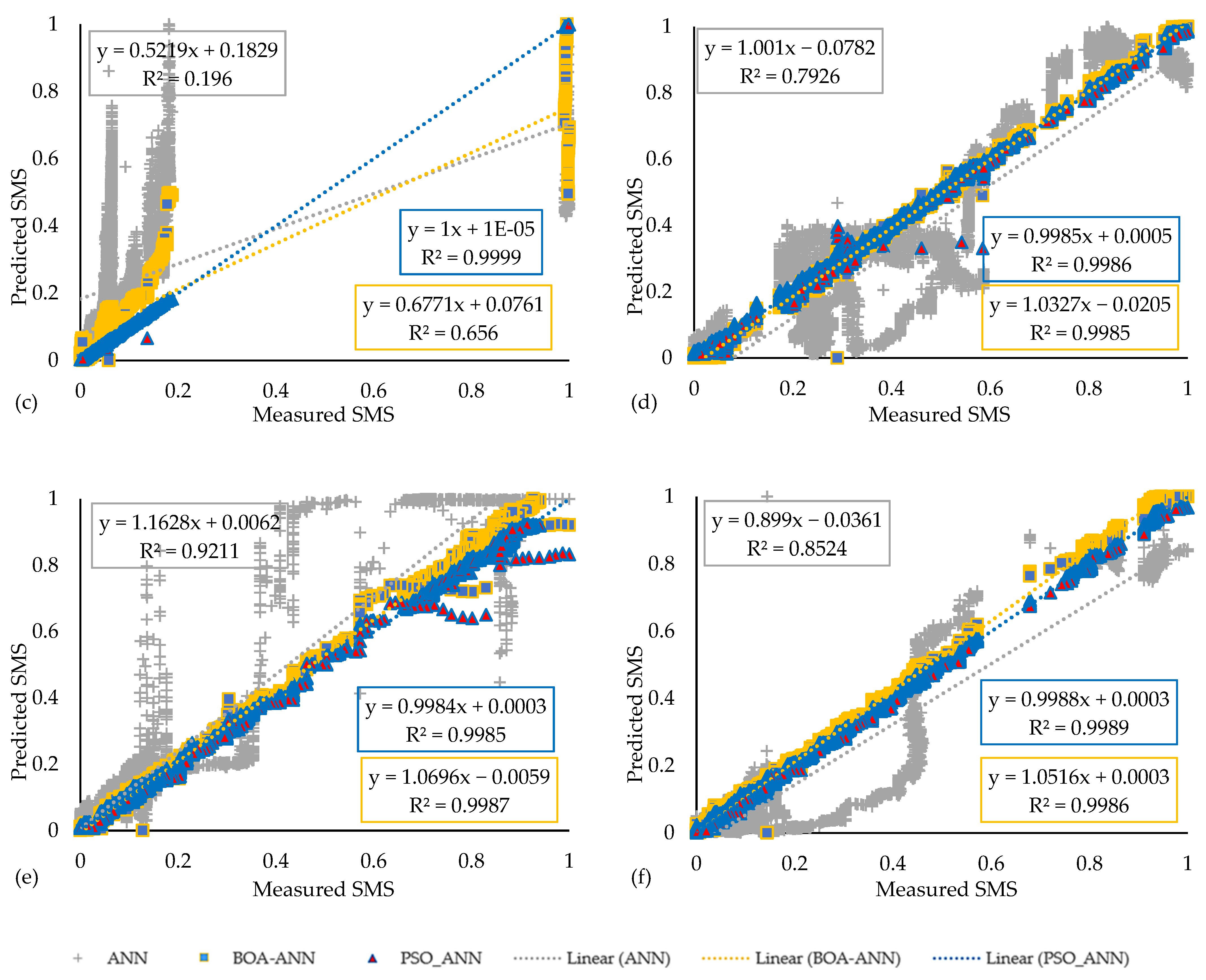
4.1. ANN-BR and Hybrid Models

Three main algorithms were used, and the result of their predictions for SMS was calculated for 1 to 18 different neurons in one hidden layer. The algorithm calculation has also been made three times for each method with varying numbers of neurons in the hidden layer. The best results of each algorithm were calculated and reported for six different HWS as well as three different depths. The ability of each model has been compared with evaluation indices. All approaches were calculated for one hidden layer and 1 to 18 numbers of neurons. The best results were reached in the higher numbers of neurons for all algorithms.

Having a better performance than ANN-LM, ANN-BR was chosen for all considered methods. For this study, the hybrid system hyperparameters were as follows: For PSO-ANN: population size: 20, iteration numbers (max): 1000, learning coefficient (both personal, (c₁) and global, (c₂) = 2, which were obtained by trial and error and resulted in the optimum values. For BOA-ANN approach: population size: 25, iteration numbers (max): 1000, switch probability value: p = 0.5, sensory modality index: c = 0.5, and power exponent: a = 0.1.

Model constraints such as slow convergence implemented local optima with stagnation and choosing random weights for connecting neurons in different layers contribute to the decline in predicted SMS in the ANN-BR. The results of the predicted and measured datasets for six HWS for three predictive approaches are shown in Figure 8, Figure A3 and Figure A4. In all Figures, the PSO-ANN results are shown in blue, BOA-ANN in yellow, and ANN-BR in gray color markers. The approach with the best result in each related HWS is shown on top of the other approaches, and regression values are shown for each method in the related HWS.

Comparing predicted and measured results, Figure 8, Figure A3 and Figure A4 present that predicted SMS values are close to the corresponding field real-time recorded data for the PSO-ANN and BOA-ANN at three different depths for all six HWS.

With R and R² near one, the best correlation between predicted and measured values can be attained. The R² statistic determines the goodness-of-fit of regression models and how well the data fit the regression model. When R² equals 0, the model cannot predict any variance in response. The PSO-ANN has precedence in R² value in two out of six HWS, and the BOA-ANN has superiority in the other four HWS at 1.5 m depth. The predicted and the measured quantities distribution shows that the ANN-BR has less performance, and hybrid intelligence models perfectly fit the regression line. The BOA-ANN model performs better in four sites out of six and is recommended for use at shallow depths (up to 1.5 m). Both hybrid algorithms’ performances are too close to each other in all HWS at 1.5 m depth, and their performance is acceptable for predicting SMS values.

The improvements in SMS prediction by using hybrid algorithms were also proven in other depths. As shown in Figure A3, PSO-ANN achieved superiority in the R² value in all HWS at 3 m depth except HWS 5 in which BOA-ANN was ranked first, and both hybrid algorithms had better performance than the ANN-BR in all HWS.

Similarly, as shown in Figure A4, in depth 4.5 m, the PSO-ANN had the best performance among the other approaches for five out of six HWS. In addition, BOA-ANN ranked first in HWS 5 and 6. Both hybrid approaches had a far better performance than the ANN-BR. In conclusion, considering the R² value, the PSO-ANN had supremacy in 12 different spots, and the BOA-ANN had superiority in 9 out of all 18 reviewed areas. It is worth mentioning that the BOA-ANN had the better performance for predicting SMS in the upper level of soil slopes (1.5 m), whereas the PSO-ANN had its best performance in both middles (3 m) and deeper levels (4.5 m) of the soil.

ANN-BR has fewer predicted SMS values because of the slow convergence pace and being trapped in local optima with stagnation. The ANN algorithm was better trained by using hybrid models. Therefore, the hybrid algorithms had a better performance in predicting SMS than the conventional ANN-BR, and they fine-tuned the ANN. Additionally, normalization before analysis prevents ANN from becoming stuck in flat regions.

Table 2. Summary of model performance indices and ranks for predictive models at 1.5 m depth.

1.5 m Depth
ANN-BR						Ranking of Each Algorithm between the Same HWS
Site Location	R	MSE	VAF	δ	#Neurons	R	MSE	VAF	δ
HWS 1	0.737496	5.50 E−03	54.389	1.082	16	3	3	3	3
HWS 2	0.997647	3.12E+00	99.530	0.100	16	3	3	3	3
HWS 3	0.948841	3.28E−02	90.024	1.768	15	3	3	3	3
HWS 4	0.684909	4.86E−02	46.870	0.889	18	3	3	3	3
HWS 5	0.691881	7.03E−01	47.866	0.254	14	3	3	3	3
HWS 6	0.963224	1.67E−02	92.742	1.839	16	3	3	3	3
PSO-ANN						Ranking of each algorithm between the same HWS
Site Location	R	MSE	VAF	δ	#Neurons	R	MSE	VAF	δ
HWS 1	0.997447	2.17E−03	99.489	1.988	16	1	1	1	1
HWS 2	0.999650	1.25E+00	99.926	0.750	17	2	2	2	2
HWS 3	0.998699	3.41E−03	99.182	1.986	18	2	2	2	2
HWS 4	0.984022	6.55E−03	88.116	1.843	16	2	2	2	2
HWS 5	0.886905	4.35E−01	78.657	1.138	16	1	2	1	2
HWS 6	0.998098	8.02E−04	99.382	1.989	18	2	1	2	2
BOA-ANN						Ranking of each algorithm between the same HWS
Site Location	R	MSE	VAF	δ	#Neurons	R	MSE	VAF	δ
HWS 1	0.996795	2.61E−03	97.626	1.967	16	2	2	2	2
HWS 2	0.999750	1.03E+00	99.945	0.969	18	1	1	1	1
HWS 3	0.999050	2.34E−03	99.260	1.988	18	1	1	1	1
HWS 4	0.993680	2.26E−03	90.077	1.886	16	1	1	1	1
HWS 5	0.840119	1.79E−01	66.443	1.191	18	2	1	2	1
HWS 6	0.999600	1.83E−03	99.601	1.993	18	1	2	1	1

The data sample size (#observations) is 13,690 for all six HWS.

,

Table A6. Summary of model performance indices and ranks for predictive models at 3 m depth.

3 m Depth
ANN-BR						Ranking of Each Algorithm between the Same HWS
Site Location	R	MSE	VAF	δ	#Neurons	R	MSE	VAF	δ
HWS 1	0.538	1.80 × 10−3	76.610	1.055	18	3	1	3	3
HWS 2	0.984	3.88 × 10−2	96.887	1.899	16	3	3	3	3
HWS 3	0.442	4.18 × 10−2	46.201	0.616	18	3	3	3	3
HWS 4	0.890	1.62 × 10−2	79.256	1.569	18	3	3	3	3
HWS 5	0.959	6.20 × 10−3	92.113	1.836	16	3	3	2	2
HWS 6	0.923	1.50 × 10−3	85.231	1.703	17	3	3	3	3
PSO-ANN						Ranking of each algorithm between the same HWS
Site Location	R	MSE	VAF	δ	#Neurons	R	MSE	VAF	δ
HWS 1	0.997	1.88 × 10−3	97.817	1.972	18	1	2	1	1
HWS 2	0.999	4.18 × 10−4	99.987	1.999	18	1	2	2	1
HWS 3	0.999	4.82 × 10−4	95.997	1.959	16	1	1	2	1
HWS 4	0.999	3.69 × 10−4	96.906	1.967	16	1	2	1	1
HWS 5	0.999	4.02 × 10−4	92.808	1.926	16	2	1	1	1
HWS 6	0.999	1.77 × 10−4	94.879	1.948	18	1	1	1	1
BOA-ANN						Ranking of each algorithm between the same HWS
Site Location	R	MSE	VAF	δ	#Neurons	R	MSE	VAF	δ
HWS 1	0.995	4.84 × 10−3	97.466	1.962	18	2	3	2	2
HWS 2	0.999	3.97 × 10−4	99.988	1.999	18	1	1	1	1
HWS 3	0.809	5.43 × 10−4	96.577	1.621	16	2	2	1	2
HWS 4	0.999	3.30 × 10−4	96.904	1.967	18	2	1	2	1
HWS 5	0.999	4.45 × 10−4	35.210	1.350	18	1	2	3	3
HWS 6	0.999	2.05 × 10−4	94.861	1.947	18	2	2	2	2

The data sample size (#observations) is 13,690 for all six HWS.

and

Table A7. Summary of model performance indices and ranks for predictive models at 4.5 m.

4.5 m Depth
ANN-BR						Ranking of EACH Algorithm between the Same HWS
Site Location	R	MSE	VAF	δ	#Neurons	R	MSE	VAF	δ
HWS 1	0.857	1.00 × 10−4	91.254	1.648	14	3	1	3	3
HWS 2	0.735	4.00 × 10−3	54.081	1.078	16	3	3	3	3
HWS 3	0.994	1.17 × 10−1	98.959	1.862	16	3	3	3	3
HWS 4	0.982	2.79 × 10−2	95.985	1.896	18	3	2	3	3
HWS 5	0.999	2.20 × 10−3	99.979	1.997	17	3	3	3	3
HWS 6	0.926	9.70 × 10−3	85.902	1.708	18	3	3	3	3
PSO-ANN						Ranking of each algorithm between the same HWS
Site Location	R	MSE	VAF	δ	#Neurons	R	MSE	VAF	δ
HWS 1	0.998	1.58 × 10−3	97.875	1.973	16	1	2	1	1
HWS 2	0.998	2.21 × 10−4	99.779	1.995	17	1	1	1	1
HWS 3	0.999	1.95 × 10−3	99.942	1.997	18	1	1	1	1
HWS 4	0.997	4.62 × 10−2	99.335	1.942	18	1	3	2	2
HWS 5	1.00	1.20 × 10−4	99.999	2.000	18	1	1	1	1
HWS 6	0.983	1.59 × 10−4	95.709	1.924	18	2	1	1	2
BOA-ANN						Ranking of each algorithm between the same HWS
Site Location	R	MSE	VAF	δ	#Neurons	R	MSE	VAF	δ
HWS 1	0.996	2.68 × 10−3	97.619	1.967	18	2	3	2	2
HWS 2	0.998	2.85 × 10−4	99.734	1.994	16	2	2	2	2
HWS 3	0.999	3.83 × 10−3	99.920	1.995	18	2	2	2	2
HWS 4	0.997	2.33 × 10−3	99.944	1.992	17	2	1	1	1
HWS 5	1.00	2.01 × 10−4	99.999	2.000	18	1	2	2	1
HWS 6	0.998	2.20 × 10−4	95.678	1.954	18	1	2	2	1

The data sample size (#observations) is 13,690 for all six HWS.

present both hybrid and ANN-BR models’ performance characteristics in terms of R, MSE, VAF, and δ at three different depths for all six HWS, signifying weak performance for ANN-BR in compare of other hybrid models. The performance quality monitoring can also be exercised by MSE, in which the real measured deviation between predicted and measured data is compared.

The Root Mean Square Error (RMSE), R², R, VAF, and $\delta$ were used to examine and to compare the predictions. It should be noted that idealistic parameters for performance indices are: $\delta$ = 2, R² = 1, RMSE = 0, and VAF = 100. The results of evaluating the indices and model ranking for the number of neurons in one hidden layer for the best scenarios for ANN-BR, PSO, and BOA algorithms are tabulated in Table 2 for 1.5 m depth and Table A6 and Table A7 for 3 m depth and 4.5 m depth, respectively. Additionally, the following performance indices were used to assess the correctness of the suggested predicted models as provided in Equations (8)–(10), where $\gamma , G, H, and n$ denote the measured, predicted, $\gamma$ ‘s mean values, and datasets total observations (recordings), respectively. As a result, a new localized performance index ($\delta$) is considered and quantified, as shown in Equation (11) and documented in [23].

Table 1 shows the statistical summary of applied methods’ performance indices in the 1.5 m depth. The PSO-ANN has the least MSE value of HWS 1 and HWS 6, and the BOA-ANN model has the best performance in other HWS at 1.5 depth.

Similarly, for the 3 m depths, the best MSE results were achieved by the hybrid approaches. According to Table A6, the PSO-ANN had the best performance in terms of the fewer MSE values for HWS 3, 5, and HWS 6. The BOA-ANN had superiority in the HWS 2 and 4 for 3.5 m depth and ANN-BR for the HWS1. Likewise, tabulated in Table A7, for the 4.5 m depth, the PSO-ANN had prevalence in all HWS except HWS 1 and four regarding the less measure of MSE, and the BOA-ANN had the better performance in HWS 4, while ANN-BR excelled in HWS 1. In total, both hybrid algorithms had a better performance than the ANN-BR. Although the best performances have been achieved with higher numbers of neurons, they take more computation time. In this study, our data analysis was extracted based on MSE. However, in order to calculate $\delta$ in Equation (11), we need RMSE along with the other performance parameters. In this study, the final evaluation of the algorithms was done based on a $\delta$ value, which tabulated for all surveyed spots in Table 2, Table A6 and Table A7. The final performance is shown in the Figure 9.

$$R^2=1-\left(\raisebox{1ex}{${{\displaystyle \sum }}_{m=1}^n{\left(\gamma -G\right)}^2$}\!\left/ \!\raisebox{-1ex}{${{\displaystyle \sum }}_{m=1}^n{\left(H\right)}^2$}\right.\right)$$

(8)

$$VAF=\left(1-\left\{\raisebox{1ex}{$var\left(\gamma -G\right)$}\!\left/ \!\raisebox{-1ex}{$var\left(\gamma \right)$}\right.\right\}\right)\times 100$$

(9)

$$RMSE=\sqrt[2]{\frac{1}{n}{{\displaystyle \sum }}_{m=1}^n{\left(\gamma -G\right)}^2}$$

(10)

$$\delta =R^2+\left(\raisebox{1ex}{$VAF$}\!\left/ \!\raisebox{-1ex}{$100$}\right.\right)-RMSE$$

(11)

The final performance evaluation of the algorithms is achieved based on a $\delta$ value by which the algorithm with the closest value to 2 has the best prediction. All $\delta$ values and algorithms rank are tabulated in Table 2 for 1.5 depth, and in Table A6 and Table A7 for 3 m and 4.5 m depths, respectively. Figure 9 shows the number of each algorithm with the first rank based on $\delta$ values, for each depth. In some HWS, PSO-ANN and BOA-ANN have the same $\delta$ values; therefore, both ranked first and counted in their final performance. As shown in Figure 9 the PSO-ANN achieved the best performance in terms of the total rank of $\delta$, and the BOA-ANN stood in the second position. Both hybrid algorithms performed better than the ANN-BR, and their performances were too close in multiple HWS. In 1.5 depth, the BOA-ANN had the best performance and ranked first in five out of six HWS. In 3 m depth, the PSO-ANN outperformed in all HWS. The BOA-ANN in HWS 2 and 4 had similar values to the PSO-ANN. Again, in-depth 4.5 m, the PSO-ANN outperformed in 4 HWS and BOA-ANN in three out of six HWS. Both hybrid algorithms had a similar performance in HWS 5. Therefore, BOA-ANN for shallow depths and PSO-ANN for deeper depths are recommended for prediction in similar cases.

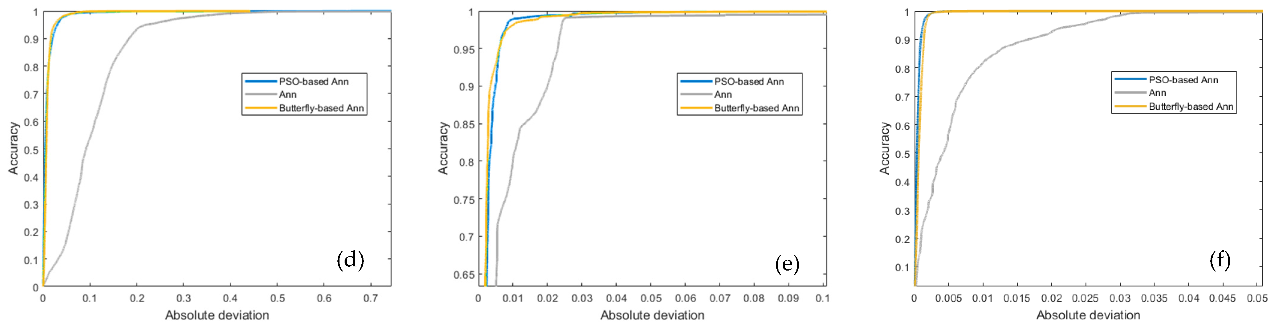
4.2. Regression Error Characteristic Curves

The Regression Error Characteristic (REC) curves illustrate the trade-off between error tolerance and functional correctness. The REC curve is a function that approximates the error cumulative distribution function [52]. It shows the error tolerance (x-axis) against the percentage of predicted points that fall inside the tolerance (y-axis). In other words, the closer the predicted values are to the upper left corner, the higher the accuracy. Also, the model’s performance can be measured by the area under the REC curve. The REC curve aims to develop a curve that analogously identifies the quality of regression models. The figure’s geometry allows for estimating regularly used distribution measures and visually depicts commonly used statistics. The generated curve approximates the error’s cumulative distribution function and enables visual comparisons between regression functions and the null model (Figure 10) [53]. The result of best performances for all hybrid intelligence models and ANN-BR are shown for three different depths. Figure 11 shows the accuracy of models for six different HWS for 1.5 m depth. The result shows hybrid models outperform the ANN-BR for predicting SMS values. The figures have been zoomed in some cases to better show the differences between algorithm performances. Figure A5 and Figure A6 consider the performance of these algorithms for 3 m and 4.5 m depths, respectively. Based on the REC results, the PSO-ANN showed the highest level of accuracy in comparison to the other two available models in all 18 different spots because it is nearer to the upper left edge, which shows the ideal performance.

4.3. Sensitivity Analysis

Yang and Zhang (1997) suggested an analytical ANN-based sensitivity method [54]. Sensitivity analysis identifies parameters and their impacts that affect the output of a dataset. Equation (12) can be used to determine the variables’ sensitivity.

$${\omega }_{kl}=\raisebox{1ex}{${{\displaystyle \sum }}_{\beta =1}^{\alpha }\left({ϵ}_{k\beta }\times {ϵ}_{l\beta }\right)$}\!\left/ \!\raisebox{-1ex}{$\sqrt{{{\displaystyle \sum }}_{\beta =1}^{\alpha }{ϵ}_{k\beta }^2{{\displaystyle \sum }}_{\beta =1}^{\alpha }{ϵ}_{l\beta }^2}$}\right.$$

(12)

where, ${ϵ}_k$,${ϵ}_l$ and $\alpha$ are the input variables, the output variables, and the total individual datasets in Equation (8). The ${\omega }_{kl}$ value is a number between 0 and 1, in which 1 indicates a high correlation between the input and output of the dataset, and 0 indicates no connection.

Figure 12, Figure A7 and Figure A8 present the input variables’ impact factor on the predicted output parameter for three proposed models in six HWS at three different depths. Based on the sensitivity analysis, it was observed that rainfall input parameters had the most impact on the output value (SMS) for the six HWS at three different depths. It was also seen that the degree of influence of the other input parameters was almost similar in six HWS at three different depths. It can be mentioned that the effectiveness of the rainfall input parameter was 3 to 4 times greater than other input variables, comparatively. In what follows, the impacts of the input variables are quantified based on the sensitivity analysis.

Based on the results, the summary of findings is presented below:

• The performance of ANN-BR in all initially calculated models was better than ANN-LM. A similar result was achieved when comparing the ANN-BR and ANN-LM in hybrid algorithms;
• The PSO-ANN was capable of accurately predicting the SMS. The PSO algorithm had the best total performance in fine-tuning ANN-BR for predicting the SMS regarding R², MSE, δ, and REC curve values. Specifically, the PSO-ANN had superiority in 11 out of 18 HWS in terms of R² value; most of them were in the deeper level of the soil slopes (3 m and 4.5 m). Regarding the R² value, the BOA-ANN dominates the four most accurate SMS predictions in the upper spots of studied soil slopes (1.5 m depth). R² values of both hybrid algorithms were too close to each other in all 18 considered spots, and both are recommended for predicting SMS;
• In terms of MSE, PSO-ANN had the better performance in HWS 1, and HWS 6 and BOA-ANN had the better performance in the remaining HWS in 1.5 depth. For the 3 m depth, the PSO-ANN had prevalence in HWS 3, 5, and HWS6, the BOA-ANN dominated the prediction of HWS 2 and HWS 4’s SMS values, and the ANN-BR had a better performance in HWS 1. For 4.5 m depth, the PSO-ANN had a better convergence in HWS 2, 3, 5, and 6, and the ANN-BR performed better in HWS 1 and BOA-ANN in HWS 4;
• From the REC values point of view, the PSO-ANN had the best performance in all 18 HWS’ SMS predictions. Both hybrid methods could escalate the effectiveness of the normal ANN-BR, and their performance had a significant privilege over the ANN-BR approach;
• Considering the combination index, δ, by which all R2, RMSE, and VAF values were considered in tandem for each algorithm, the performance of the PSO-ANN was better in HWS 1; for the BOA-ANN in HWS 2, 3, 4, 5, and 6 at 1.5 m depth. At 3 m depth, the PSO-ANN model had the best performance in all HWS, and the BOA-ANN had a similar performance in HWS 2 and 4. Similarly, for 4 m depth, the PSO-ANN had the best performance in HWS 1, 2, 3, and 5, and the BOA-ANN had a better performance in HWS 4, 5, and 6. Both hybrid algorithms had similar performance for HWS 5;
• Regarding input variables, inserting the soil and air temperature data sets had a crucial impact on the accuracy of SMS prediction. After adding these two variables’ data sets, the accuracy of the predicted ANN-BR model improved by 30%;
• All input variables, such as soil temperature, VSMC, rainfall, and the air temperature influence predicting SMS. In sensitivity analysis, the rainfall variable with the highest impact on SMS and its effectiveness was 3 to 4 times more than other input variables;
• As a result, the hybrid models proposed in this work have the potential to be implemented as a precise technique for SMS prediction and fine-tuning the ANN-BR algorithm.

5. Discussion

The hybrid intelligent training approach is one of the most extensively used ways of training artificial neural networks [30,31,38,55]. Besides two-hybrid approaches for predicting SMS, the conventional ANN-BR was also used as a competitor in this research due to its ability to predict values with fair results and errors. When comparing prediction performance indices, the ANN-BR was the only model with the most difference in the target variable. The results of an ANN-BR and the proposed hybrid intelligent models are very different from each other (Table 2, Table A6 and Table A7). Therefore, metaheuristic algorithms can be used to justify altering the neural network weights and biases during the training and testing phases. The performance indices show that the acquired results of the PSO-ANN in predicting SMS are highly correlated by which model can predict SMS with a high degree of accuracy in all six HWS datasets used in this study.

Moreover, the field instrumented plan was chosen based on the parameters that affect the stability of the HWS. For example, rainfall volume impacts the VSMC, and soil and air temperatures contribute to the propagation of soil cracks based on seasonal changes induced by vertical permeability variation. The SMS can be determined from the VSMC using the SWRC. Knowing the SMS, an indicator of the soil shear strength allows for evaluating the HWS’s performance based on its stable condition. Now, we can see how the SMS prediction can indirectly assess the HWS stability conditions.

The hybrid algorithms predict the values within a specified time interval, a process known as ANN-based prediction and ANN-based interpolation. This does not imply extrapolation or forecasting. Both interpolation and prediction techniques, however, are useful.

The variation of SMS values at each depth and each HWS is different. In other words, there seems to be a noticeable difference between predicted and measured SMS values in a few HWS, such as HWS 5. This difference could be attributed to many geotechnical parameters, conditions, and loadings. The reasons are a combination of different components such as a high volume of precipitation, temporal seasonal variations, soil body movement, development of perched water zones, development of cracks, soil body fully saturated condition, and other impacting factors. That is why in some cases, it was observed that we had lower accuracy and more accumulation (congestion) of data points in a specific zone.

In addition, the primary focus of this study was on the category of ANN-based back-propagation training algorithms, their combination with metaheuristic algorithms, and optimizing the weights and biases of ANN-BR in combination with metaheuristic algorithms. Due to the great number of data records, which takes time for each iteration to evaluate in similar conditions for six HWS at each depth, the Recurrent Neural Networks (RNN), Long Short-Term Memory (LSTM), and similar approaches were not considered in the scope of this research. Using RNN or different techniques, such as the LSTM with feed-forward training algorithms, is recommended for future research.

Figure 13 shows susceptible regions of expansive clay soil with different degrees to apply the proposed model of this research. The red color indicated the high expansive clay zones. Our referenced slopes are precisely sitting on the red color zones and have shown early signs of movement, so we selected these HWS zones [56]. The index properties of the red color soil our reference HWS are made of are as follows; Liquid Limit >80 and percent of volume change >200. All regions in the US and outside of the US with these mentioned soil index properties could be included for implementing the proposed model in this study. There are so many uncertainties in geotechnical engineering. If the models might not be perfectly matched for other regions, they could be implemented for the initial and pre-evaluation analyses.

6. Conclusions

In this study, the feasibility of hybrid artificial intelligence systems and the simplicity of the ANN were considered in the prediction of SMS. A total of three intelligent prediction systems, namely the ANN-BR, PSO-ANN, and BOA-ANN, were developed to predict the SMS variation at three different depths in six HWS constructed of HVCCS using air temperature, soil temperature, VSMC, and rainfall as input variables. Field data was gathered from six monitoring locations in the Mississippi, all of which were near the Jackson Metropolitan Area. Three models were developed to predict the SMS of the HVCCS using 13,690 hourly data records for each of the input variables at every six HWS. Taking into account a variety of performance indices, a thorough comparison of the previously described predictive approaches was conducted in order to determine the most effective model for predicting the SMS.

In standard ANN models, the initial weights of the input variables, hidden layers, and output variables are determined randomly, and the weights are optimized during the training phase. The weights and biases used in the ANN significantly impact its output and accuracy. By modifying weights and biases, predictive ANN-based algorithms can minimize cost functions. This research used PSO-ANN and BOA-ANN with a different 1 to 18 neurons to optimize ANN weights and biases. It is worth mentioning that among all the other available methods, ANN was selected due to its acceptability in the majority of research work, low processing time, ability to quickly deliver validated results, compatibility with other methods, and fast learning factor. Advance hybrid approaches were used, which are more powerful in terms of real-time prediction and more efficient for fine-tuning ANN and analysis of the proposed method.

Performance indices showed that the PSO-ANN had the best prediction for SMS in Yazoo clay soil in six HWS in metropolitan Jackson and ranked first in 11 of 18 surveyed soil spots. The BOA-ANN ranked as the second-best approach and outperformed in 9 of 18 soil areas. In some areas, both hybrid approaches had a similar performance and ranked as the best approach together. In addition, the BOA-ANN had the best performance in shallow levels, and the PSO-ANN predicted SMS better in the deeper soil levels.

This study showed that air temperature, soil temperature, rainfall, and VSMC influence predicting SMS, and rainfall had the greatest influence among other input variables.

In the end, by considering such hybrid approaches, the ANN can be fine-tuned; hence, the soil matric interaction can be better understood. This type of research helps to move forward using interpolation and extrapolation techniques to predict the soil matric values and therefore predict possible landslides with a higher level of accuracy, especially in susceptible areas. Considering the economic and human losses in a landslide on highways and natural slopes, predicting and taking ad hoc action would be a preventive response to these natural disasters. Performing predictive and preventative maintenance and using other machine learning approaches for other types of soils are recommended for future work.

References

1. Douglas, S.; Dunlap, G. Light commercial construction on Yazoo clay. Forensic Eng. 2000, 2000, 607–616. [Google Scholar]
2. Lee, L.T., Jr. State Study 151 and 236: Yazoo Clay Investigation; Transportation Research Record (TRR): Thousand Oaks, CA, USA, 2012. [Google Scholar]
3. Khan, M.S.; Amini, F.; Nobahar, M. Performance Evaluation of Highway Slopes on Yazoo Clay; Mississippi. Dept. of Transportation: Washington, DC, USA, 2020.
4. Cai, J.-S.; Yeh, T.-C.J.; Yan, E.-C.; Tang, R.-X.; Hao, Y.-H.; Huang, S.-Y.; Wen, J.-C. Importance of variability in initial soil moisture and rainfalls on slope stability. J. Hydrol. 2019, 571, 265–278. [Google Scholar] [CrossRef]
5. Melinda, F.; Rahardjo, H.; Han, K.K.; Leong, E.C. Shear strength of compacted soil under infiltration condition. J. Geotech. Geoenviron. Eng. 2004, 130, 807–817. [Google Scholar] [CrossRef]
6. Lim, T.; Rahardjo, H.; Chang, M.; Fredlund, D.G. Effect of rainfall on matric suctions in a residual soil slope. Can. Geotech. J. 1996, 33, 618–628. [Google Scholar] [CrossRef]
7. Kaykhosravi, S.; Khan, U.T.; Jadidi, M.A. The effect of climate change and urbanization on the demand for low impact development for three Canadian cities. Water 2020, 12, 1280. [Google Scholar] [CrossRef]
8. Marengo, J.A.; Camarinha, P.I.; Alves, L.M.; Diniz, F.; Betts, R.A. Extreme rainfall and hydro-geo-meteorological disaster risk in 1.5, 2.0, and 4.0 °C global warming scenarios: An analysis for Brazil. Front. Clim. 2021, 3, 610433. [Google Scholar] [CrossRef]
9. Mallick, J.; Alqadhi, S.; Talukdar, S.; AlSubih, M.; Ahmed, M.; Khan, R.A.; Kahla, N.B.; Abutayeh, S.M. Risk assessment of resources exposed to rainfall induced landslide with the development of GIS and RS based ensemble metaheuristic machine learning algorithms. Sustainability 2021, 13, 457. [Google Scholar] [CrossRef]
10. Touma, D.; Stevenson, S.; Swain, D.L.; Singh, D.; Kalashnikov, D.A.; Huang, X. Climate change increases risk of extreme rainfall following wildfire in the western United States. Science advances 2022, 8, eabm0320. [Google Scholar] [CrossRef]
11. Kaykhosravi, S.; Abogadil, K.; Khan, U.T.; Jadidi, M.A. The low-impact development demand index: A new approach to identifying locations for LID. Water 2019, 11, 2341. [Google Scholar] [CrossRef] [Green Version]
12. Kaykhosravi, S.; Khan, U.T.; Jadidi, M.A. A simplified geospatial model to rank LID solutions for urban runoff management. Sci. Total Environ. 2022, 831, 154937. [Google Scholar] [CrossRef]
13. Duncan, J.M.; Wright, S.G.; Brandon, T.L. Soil Strength and Slope Stability; John Wiley & Sons: Hoboken, NJ, USA, 2014. [Google Scholar]
14. Statistics Bureau of Transportation. National Transportation Statistics. Res. Innov. Technol. Adm. 2015, 1–470. [Google Scholar]
15. International Traffic Safety Data and Analysis Group. Road Safety Annual Report; International Traffic Safety Data and Analysis Group: Paris, France, 2019. [Google Scholar]
16. Fassin, D.; Vasquez, P. Humanitarian exception as the rule: The political theology of the 1999 Tragedia in Venezuela. Am. Ethnol. 2005, 32, 389–405. [Google Scholar] [CrossRef]
17. Kothari, U.C.; Momayez, M. Machine learning: A novel approach to predicting slope instabilities. Int. J. Geophys. 2018, 2018, 4861254. [Google Scholar] [CrossRef] [Green Version]
18. Haykin, S.; Network, N. A comprehensive foundation. Neural Netw. 2004, 2, 41. [Google Scholar]
19. Nie, W.; Feng, D.; Lohpaisankrit, W.; Li, C.; Yuan, J.; Chen, Y. A dynamic Bayesian network-based model for evaluating rainfall-induced landslides. Bull. Eng. Geol. Environ. 2019, 78, 2069–2080. [Google Scholar] [CrossRef]
20. Wang, Y.; Aladejare, A.E. Bayesian characterization of correlation between uniaxial compressive strength and Young’s modulus of rock. Int. J. Rock Mech. Min. Sci. 2016, 85, 10–19. [Google Scholar] [CrossRef]
21. Xu, Y.; Zhang, L.; Jia, J. Diagnosis of embankment dam distresses using Bayesian networks. Part II. Diagnosis of a specific distressed dam. Can. Geotech. J. 2011, 48, 1645–1657. [Google Scholar] [CrossRef]
22. Araei, A.A. Artificial neural networks for modeling drained monotonic behavior of rockfill materials. Int. J. Geomech. 2014, 14, 04014005. [Google Scholar] [CrossRef]
23. Yagiz, S.; Sezer, E.; Gokceoglu, C. Artificial neural networks and nonlinear regression techniques to assess the influence of slake durability cycles on the prediction of uniaxial compressive strength and modulus of elasticity for carbonate rocks. Int. J. Numer. Anal. Methods Geomech. 2012, 36, 1636–1650. [Google Scholar] [CrossRef]
24. Shahin, M.A.; Maier, H.R.; Jaksa, M.B. Data division for developing neural networks applied to geotechnical engineering. J. Comput. Civ. Eng. 2004, 18, 105–114. [Google Scholar] [CrossRef]
25. Nobahar, M.; Khan, M. Prediction of Matric Suction of Highway Slopes Using Autoregression Artificial Neural Network (ANN) Model. Geo-Extreme 2021, 2021, 40–50. [Google Scholar]
26. Snieder, E.; Khan, U. Large-Scale Evaluation of Temporal Trends in ANN Behaviour for Daily Flow Forecasts in Canadian Catchments. In Proceedings of the EGU General Assembly 2022, Vienna, Austria, 23–27 May 2022. [Google Scholar]
27. Khan, U.T.; He, J.; Valeo, C. River flood prediction using fuzzy neural networks: An investigation on automated network architecture. Water Sci. Technol. 2018, 2017, 238–247. [Google Scholar] [CrossRef] [PubMed]
28. Liou, Y.-A.; Liu, S.-F.; Wang, W.-J. Retrieving soil moisture from simulated brightness temperatures by a neural network. IEEE Trans. Geosci. Remote Sens. 2001, 39, 1662–1672. [Google Scholar]
29. Atluri, V.; Hung, C.-C.; Coleman, T.L. An artificial neural network for classifying and predicting soil moisture and temperature using Levenberg-Marquardt algorithm. In Proceedings of the IEEE Southeastcon’99. Technology on the Brink of 2000 (Cat. No. 99CH36300), Lexington, Kentucky, 25–28 March 1999; pp. 10–13. [Google Scholar]
30. Moayedi, H.; Mehrabi, M.; Mosallanezhad, M.; Rashid, A.S.A.; Pradhan, B. Modification of landslide susceptibility mapping using optimized PSO-ANN technique. Eng. Comput. 2019, 35, 967–984. [Google Scholar] [CrossRef]
31. Taghizadeh-Mehrjardi, R.; Emadi, M.; Cherati, A.; Heung, B.; Mosavi, A.; Scholten, T. Bio-inspired hybridization of artificial neural networks: An application for mapping the spatial distribution of soil texture fractions. Remote Sens. 2021, 13, 1025. [Google Scholar] [CrossRef]
32. Gordan, B.; Jahed Armaghani, D.; Hajihassani, M.; Monjezi, M. Prediction of seismic slope stability through combination of particle swarm optimization and neural network. Eng. Comput. 2016, 32, 85–97. [Google Scholar] [CrossRef]
33. Asadnia, M.; Chua, L.H.; Qin, X.; Talei, A. Improved particle swarm optimization–based artificial neural network for rainfall-runoff modeling. J. Hydrol. Eng. 2014, 19, 1320–1329. [Google Scholar] [CrossRef]
34. Alqadhi, S.; Mallick, J.; Talukdar, S.; Bindajam, A.A.; Saha, T.K.; Ahmed, M.; Khan, R.A. Combining logistic regression-based hybrid optimized machine learning algorithms with sensitivity analysis to achieve robust landslide susceptibility mapping. Geocarto Int. 2021, 1–26. [Google Scholar] [CrossRef]
35. Paryani, S.; Neshat, A.; Javadi, S.; Pradhan, B. Comparative performance of new hybrid ANFIS models in landslide susceptibility mapping. Nat. Hazards 2020, 103, 1961–1988. [Google Scholar] [CrossRef]
36. Nguyen, H.; Mehrabi, M.; Kalantar, B.; Moayedi, H.; Abdullahi, M.a.M. Potential of hybrid evolutionary approaches for assessment of geo-hazard landslide susceptibility mapping. Geomat. Nat. Hazards Risk 2019, 10, 1667–1693. [Google Scholar] [CrossRef]
37. Bui, D.T.; Moayedi, H.; Kalantar, B.; Osouli, A.; Pradhan, B.; Nguyen, H.; Rashid, A.S.A. A novel swarm intelligence—Harris hawks optimization for spatial assessment of landslide susceptibility. Sensors 2019, 19, 3590. [Google Scholar] [CrossRef] [PubMed] [Green Version]
38. Rukhaiyar, S.; Alam, M.; Samadhiya, N.K. A PSO-ANN hybrid model for predicting factor of safety of slope. Int. J. Geotech. Eng. 2018, 12, 556–566. [Google Scholar] [CrossRef]
39. Xi, W.; Li, G.; Moayedi, H.; Nguyen, H. A particle-based optimization of artificial neural network for earthquake-induced landslide assessment in Ludian county, China. Geomat. Nat. Hazards Risk 2019, 10, 1750–1771. [Google Scholar] [CrossRef] [Green Version]
40. Xing, Y.; Yue, J.; Chen, C. Interval estimation of landslide displacement prediction based on time series decomposition and long short-term memory network. IEEE Access 2019, 8, 3187–3196. [Google Scholar] [CrossRef]
41. Zhang, D.; Liu, J.; He, X.; Yang, L.; Cui, T.; Yu, T.; Kheiry, A.N. Application of swarm intelligence algorithms to the characteristic wavelength selection of soil moisture content. Int. J. Agric. Biol. Eng. 2021, 14, 153–161. [Google Scholar] [CrossRef]
42. Lohar, G.; Sharma, S.; Saha, A.K.; Ghosh, S. Optimization of geotechnical parameters used in slope stability analysis by metaheuristic algorithms. In Applications of Internet of Things; Springer: Berlin/Heidelberg, Germany, 2021; pp. 223–231. [Google Scholar]
43. Yitian, L.; Gu, R.R. Modeling flow and sediment transport in a river system using an artificial neural network. Environ. Manag. 2003, 31, 0122–0134. [Google Scholar] [CrossRef]
44. Wilby, R.L.; Wigley, T.; Conway, D.; Jones, P.; Hewitson, B.; Main, J.; Wilks, D. Statistical downscaling of general circulation model output: A comparison of methods. Water Resour. Res. 1998, 34, 2995–3008. [Google Scholar] [CrossRef]
45. Bishop, C.M. Neural networks and their applications. Rev. Sci. Instrum. 1994, 65, 1803–1832. [Google Scholar] [CrossRef] [Green Version]
46. O’Shea, K.; Nash, R. An introduction to convolutional neural networks. arXiv 2015, arXiv:1511.08458. [Google Scholar]
47. Nielsen, M.A. Neural Networks and Deep Learning; Determination Press: San Francisco, CA, USA, 2015; Volume 25. [Google Scholar]
48. Kennedy, J.; Eberhart, R. Particle swarm optimization. In Proceedings of the ICNN’95-International Conference on Neural Networks, Perth, WA, Australia, 27 November–1 December 1995; pp. 1942–1948. [Google Scholar]
49. Kennedy, J.; Eberhart, R.C. A discrete binary version of the particle swarm algorithm. In Proceedings of the 1997 IEEE International Conference on Systems, Man, and Cybernetics. Computational Cybernetics and Simulation, Orlando, FL, USA, 12–15 October 1997; pp. 4104–4108. [Google Scholar]
50. Stevens, S.S.; Marks, L.E. Psychophysics: Introduction to Its Perceptual, Neural, and Social Prospects; Routledge: London, UK, 2017. [Google Scholar]
51. Arora, S.; Singh, S. Butterfly optimization algorithm: A novel approach for global optimization. Soft Comput. 2019, 23, 715–734. [Google Scholar] [CrossRef]
52. Arora, S.; Anand, P. Learning automata-based butterfly optimization algorithm for engineering design problems. Int. J. Comput. Mater. Sci. Eng. 2018, 7, 1850021. [Google Scholar] [CrossRef]
53. Bi, J.; Bennett, K.P. Regression error characteristic curves. In Proceedings of the 20th International Conference on Machine Learning (ICML-03), Washington, DC, USA, 21–24 August 2003; pp. 43–50. [Google Scholar]
54. Yang, Y.; Zhang, Q. A hierarchical analysis for rock engineering using artificial neural networks. Rock Mech. Rock Eng. 1997, 30, 207–222. [Google Scholar] [CrossRef]
55. Le, L.T.; Nguyen, H.; Dou, J.; Zhou, J. A comparative study of PSO-ANN, GA-ANN, ICA-ANN, and ABC-ANN in estimating the heating load of buildings’ energy efficiency for smart city planning. Appl. Sci. 2019, 9, 2630. [Google Scholar] [CrossRef] [Green Version]
56. Olive, W.; Chleborad, A.; Frahme, C.; Schlocker, J.; Schneider, R.; Schuster, R. Swelling Clays Map of the Conterminous United States; United States Geological Survey: Reston, VA, USA, 1989.
Figure 1. Typical shallow to deep slope failures on HVCCS in Mississippi.
Mathematics 10 02825 g001
Figure 2. HWS locations (Reference Sites), Jackson.
Mathematics 10 02825 g002
Figure 3. Instrumentation layout at each HWS and Image of the Individual Sensors.
Mathematics 10 02825 g003
Figure 4. 3D in situ variation of rainfall, SMS, and VSMC at 1.5 m depth (a) HWS 1 (b) HWS 2 (c) HWS 3 (d) HWS 4 (e) HWS 5 (f) HWS 6.
Mathematics 10 02825 g004
Figure 5. Validation of VSMC Lab measured versus sensor reading.
Mathematics 10 02825 g005
Figure 6. Schematic representation of the predictive ANN-BR mode.
Mathematics 10 02825 g006
Figure 7. The modeling procedure of the hybrid PSO-ANN and BOA-ANN flowchart.
Mathematics 10 02825 g007
Figure 8. Predicted vs. measured SMS at 1.5 m depth overtime via ANN-BR model, PSO-ANN model, and BOA-ANN model along with the impact of the number of iterations on the predictive model response (a) HWS 1 (b) HWS 2 (c) HWS 3 (d) HWS 4 (e) HWS 5 (f) HWS 6.
Mathematics 10 02825 g008aMathematics 10 02825 g008b
Figure 9. Number of achieving the first rank of δ value among other algorithms in all surveyed spots.
Mathematics 10 02825 g009
Figure 10. Detailed representation of REC curves.
Mathematics 10 02825 g010
Figure 11. REC curves for the ANN-BR, PSO-ANN, and BOA-ANN for (a) HWS 1 (b) HWS 2 (c) HWS 3 (d) HWS 4 (e) HWS 5 (f) HWS 6 at 1.5 m depth.
Mathematics 10 02825 g011aMathematics 10 02825 g011b
Figure 12. The sensitivity factor of input parameters on the predicted output for the ANN-BR, PSO-ANN, and BOA-ANN at 1.5 m depth (a) HWS 1 (b) HWS 2 (c) HWS 3 (d) HWS 4 (e) HWS 5 (f) HWS 6.
Mathematics 10 02825 g012
Figure 13. U.S distribution map of expansive clay [56].
Mathematics 10 02825 g013