Mathematical Modelling of Harmful Algal Blooms on West Coast of Sabah

Abstract

Algal bloom is a condition in which there is a massive growth of algae in a certain region and it is said to be harmful when the bloom causes damage effects. Due to the tremendous impact of harmful algal bloom (HAB) on some aspects, this research proposes the mathematical modelling of an HAB model to describe the process of HAB together with population dynamics. This research considers the delay terms in the modelling since the liberation of toxic chemicals by toxin-producing phytoplankton (TPP) is not an instantaneous process in which the species need to achieve their maturity. A model of fish interaction is also being studied to show the effect of HAB on fish species. Time delay is incorporated for the mortality of fish due to the consumption of toxic zooplankton. Stability analysis is conducted and numerical simulations are applied to obtain the analytical results which highlight the critical values for the delay parameters. The existence of Hopf bifurcation is established when the delay passes the threshold value. The results of both models show that the inclusion of the delay term affects the model by stabilizing and destabilizing the model. Therefore, this research shows the effect of an inclusion delay term on the model and also gives knowledge and an understanding of the process of HAB occurrence as well as the effect of HAB on fish populations.

1. Introduction

Algal bloom is a situation wherein there is an abundance of algal cell density in a location of coastal water which is usually dominated by a single species or a few species. It is called harmful algal bloom (HAB) when the bloom has adverse effects on the marine ecosystem as well as on humans due to the natural toxin content in their body. HABs in Malaysian waters are quite worrying nowadays since the occurrence of blooms has been increasingly reported over the last decade. The natural toxins produced by the algal bloom may harm the marine ecosystem because it will accumulate in the filter-feeder shellfish and cause food poisoning to the human when they consumed shellfish.

Massive algal bloom can also kill fish or shrimp because they can barely breathe in the water to survive. High densities of algal blooms in water causes dissolved oxygen depletion. For example, in 2005, a fish killing event was reported in Penang which amounted to more than MYR 20 million in losses [1]. Therefore, it is necessary to have a good understanding and wide view of HAB dynamics and the study of marine plankton ecology is an important consideration.

HABs have regularly occurred in Sabah as early as 1976 eutrophication makes this area environmentally favourable for dinoflagellate to reproduce and grow. The water tends to be discoloured or murky, appearing red or green in colour and sometimes purple. The species of dinoflagellate that always causes bloom in Sabah seas is Pyrodinium bahamense. Whatever feeds on P. bahamense accumulates PSTs transferred from the dinoflagellates. Toxic phytoplankton do not harm shellfish but can harm humans that have consumed the contaminated shellfish. It has been yearly reported that PSP in Sabah has been caused by toxins from P. bahamense. Some filter feeder fish such as “ikan tamban, ikan basung” and “ikan rumahan” take in the dinoflagellates as well when they feed on the zooplankton.

A broad classification of HABs species distinguishes two groups: (1) the toxin producers which can contaminate seafood and kill fish; (2) the high-biomass producers which are always associated with water discolouration (red tide) that can be caused hypoxia/anoxia and subsequently have a fatal impact on marine life after reaching dense concentrations [2]. Pyrodinium bahamense is a well-known marine dinoflagellate and producer of paralytic shellfish toxin (PST) that is especially present in tropical waters [3], and which has caused more human illnesses and fatalities than any other PST-producing dinoflagellates. P. bahamense was first reported in 1976 along a 300-km-long stretch west coast of Sabah, Malaysia [4], and formed a toxic bloom in the Brunei Bay, Sabah, and resulted in human poisoning involving 202 people, with 7 casualties [4] due to paralytic shellfish poisoning (PSP). Toxic dinoflagellate P. bahamense has been a causative species for the occurrence of PSP events in Sabah annually since then [3,5,6].

Phytoplankton consists of two types which are toxic phytoplankton (TPP) and non-toxic phytoplankton (NTP). TPP have the ability to produce ‘toxic’ or ‘allelopathic agents’ that could harm the growth of other aquatic organisms [7,8], while NTP do not produce any toxic chemicals. NTP will become harmful if there is massive algal bloom that could cause a red tide. For example, when masses of algae die and decompose, the decaying process can deplete oxygen in the water, causing the water to become so low in oxygen that animals either leave the area or die. As such, phytoplankton could act as the indicator of the water quality as massive algae bloom will degrade the water quality [9].

HAB occurrences have recently alarmed the authorities to realize the need to raise awareness of HABs in Malaysia. For example, on 11th February 2014, due to the HAB bloom in Tanjung Kupang, there were massive fish kills and the operators reported losses of MYR 150,000. Fish stocks such as those of snappers, cods, seabass and threadfins in nine farms were wiped out during the event [10]. In Penang, the aquaculture operators also reported losses estimated around MYR 20 millions due to the fish kills during the period 2005–2006 [10]. Therefore, these losses could be prevented if there is an adequate monitoring program held by the relevant authorities. In addition to that, the safety of our seafood could also be guaranteed as well as our public health.

2. Materials and Methods

2.1. Nutrient-Phytoplankton-Zooplankton Interaction Model

Many researchers have constructed and studied the mathematical model of nutrient–phytoplankton–zooplankton interaction with different degrees of complexity. Mathematical modelling is important in order to improve our knowledge and understanding of the occurrence of HAB in relation to plankton ecology. This research incorporates a delay model to describe how toxin production by TPP is not an instantaneous process. This model explains how Pyrodinium bahamense sp. can cause HAB to occur.

$$\begin{array}{cc}\hfill \frac{dN}{dt}& =D(N_0-N)-{\alpha }_1{P}_{1}N-{\alpha }_2{P}_{2}N\hfill \\ \hfill \frac{d{P}_1}{dt}& ={\theta }_1{P}_{1}N-{\beta }_1{P}_1{P}_3-m_1{P}_1-e_1{P}_1{P}_2-D_1{P}_1\hfill \\ \hfill \frac{d{P}_2}{dt}& ={\theta }_2{P}_{2}N-{\beta }_2{P}_2{P}_3-m_2{P}_2-e_2{P}_1{P}_2-D_2{P}_2\hfill \\ \hfill \frac{d{P}_3}{dt}& ={\gamma }_1{P}_1{P}_3-{\gamma }_2{P}_2(t-\tau )P_3-m_3{P}_3-D_3{P}_3\hfill \end{array}$$

(1)

where

$$\begin{array}{cc}\hfill {\alpha }_1& =\mathrm{Nutrient}\mathrm{uptake}\mathrm{rate}\mathrm{for}\mathrm{the}\mathrm{NTP}\hfill \\ \hfill {\alpha }_2& =\mathrm{Nutrient}\mathrm{uptake}\mathrm{rate}\mathrm{for}\mathrm{the}\mathrm{TPP}\hfill \\ \hfill {\theta }_1& =\mathrm{Conversion}\mathrm{rate}\mathrm{of}\mathrm{NTP}\mathrm{for}\mathrm{nutrient}\hfill \\ \hfill {\theta }_2& =\mathrm{Conversion}\mathrm{rate}\mathrm{of}\mathrm{TPP}\mathrm{for}\mathrm{nutrient}\hfill \\ \hfill {\beta }_1& =\mathrm{Predation}\mathrm{rate}\mathrm{of}\mathrm{NTP}\mathrm{for}\mathrm{zooplankton}\hfill \\ \hfill {\beta }_2& =\mathrm{Predation}\mathrm{rate}\mathrm{of}\mathrm{TPP}\mathrm{for}\mathrm{zooplankton}\hfill \\ \hfill {\gamma }_1& =\mathrm{Conversion}\mathrm{rate}\mathrm{of}\mathrm{zooplankton}\mathrm{for}\mathrm{NTP}\hfill \\ \hfill {\gamma }_2& =\mathrm{Death}\mathrm{rate}\mathrm{due}\mathrm{to}\mathrm{consumption}\mathrm{of}\mathrm{TPP}\hfill \\ \hfill m_1& =\mathrm{Natural}\mathrm{death}\mathrm{rate}\mathrm{of}\mathrm{NTP}\hfill \\ \hfill m_2& =\mathrm{Natural}\mathrm{death}\mathrm{rate}\mathrm{of}\mathrm{TPP}\hfill \\ \hfill m_3& =\mathrm{Natural}\mathrm{death}\mathrm{rate}\mathrm{of}\mathrm{zooplankton}\hfill \\ \hfill D& =\mathrm{Dilution}\mathrm{rate}\mathrm{of}\mathrm{nutrient}\hfill \\ \hfill D_1& =\mathrm{Dilution}\mathrm{rate}\mathrm{of}\mathrm{NTP}\hfill \\ \hfill D_2& =\mathrm{Dilution}\mathrm{rate}\mathrm{of}\mathrm{TPP}\hfill \\ \hfill D_3& =\mathrm{Dilution}\mathrm{rate}\mathrm{of}\mathrm{zooplankton}\hfill \\ \hfill e_1& =\mathrm{Competition}\mathrm{coefficient}\mathrm{for}\mathrm{NTP}\hfill \\ \hfill e_2& =\mathrm{Competition}\mathrm{coefficient}\mathrm{for}\mathrm{TPP}\hfill \end{array}$$

• Time lag is considered for the maturation of the TPP population to produce toxin since the process is not instantaneous [3,11]. The mortality of the zooplankton population is described as $P_2(t-\tau )P_3$ [12,13].
• The functional response of Holling type I is applied for the functional response of phytoplankton to nutrients as it is used for lower organisms such as alga [14,15,16].
• The linear mass action law is used for the maximal zooplankton predation rate for NTP and TPP [17].
• The model considered interspecies competition to obtain nutrients [17].
• TPP do not harm NTP even though these contains high toxins at that time because the toxins do not secrete out into the environment [3,11,18].
• TPP harm the zooplankton whenever they are consumed and the toxin content is produced at a high level [18].

The system in (1) is rescaled by introducing new variables where

$$\begin{array}{cccccccc}\hfill x& =\frac{N}{N_0},\hfill & \hfill y& =\frac{P_1{\alpha }_1}{D},\hfill & \hfill z& =\frac{P_2{\alpha }_2}{D},\hfill & \hfill w& =\frac{P_3{\beta }_1}{D},\hfill \\ \hfill a& =\frac{{\theta }_1}{{\alpha }_1},\hfill & \hfill b& =\frac{m_1}{D},\hfill & \hfill c& =\frac{e_1}{{\alpha }_2},\hfill & \hfill d& =\frac{D_1}{D},\hfill \\ \hfill f& =\frac{{\theta }_2}{{\alpha }_2},\hfill & \hfill g& =\frac{m_2}{D},\hfill & \hfill h& =\frac{{\beta }_2}{{\beta }_1},\hfill & \hfill m& =\frac{e_1}{{\alpha }_1},\hfill \\ \hfill n& =\frac{D_2}{D},\hfill & \hfill p& =\frac{{\gamma }_1}{{\alpha }_1},\hfill & \hfill q& =\frac{{\gamma }_2}{{\alpha }_2},\hfill & \hfill r& =\frac{m_3}{D},\hfill \\ \hfill s& =\frac{D_3}{D}\hfill \end{array}$$

Then system (1) becomes

$$\begin{array}{cc}\hfill \frac{dx}{dt}& =1-x-xy-xz\hfill \\ \hfill \frac{dy}{dt}& =axy-wy-by-cyz-dy\hfill \\ \hfill \frac{dz}{dt}& =fxz-gz-hwz-myz-nz\hfill \\ \hfill \frac{dw}{dt}& =pyw-qz(t-\tau )w-rw-sw\hfill \end{array}$$

(2)

System (2) is linearized at $E^{*}=(x^{*},y^{*},z^{*},w^{*})$, in the form

$$\frac{dX}{dt}=MX\left(t\right)+NX(t-\tau )$$

(3)

where

$$M=\left[\begin{array}{cccc}{H}_1& -x^{*}& -x^{*}& 0\\ a{y}^{*}& H_2& -c{y}^{*}& -y^{*}\\ f{z}^{*}& -m{z}^{*}& H_3& -h{z}^{*}\\ 0& p{w}^{*}& 0& H_4\end{array}\right],$$

(4)

$$N=\left[\begin{array}{cccc}0& 0& 0& 0\\ 0& 0& 0& 0\\ 0& 0& 0& 0\\ 0& 0& q{w}^{*}& 0\end{array}\right]$$

(5)

and $X(.)={(x(.),y(.),z(.))}^T$ is the state vector. The characteristic equation of (3) is as follows:

$$det(\lambda -M-N{e}^{-\lambda {\tau }_1})=0$$

(6)

which can be explicitly expressed as

$$F(\lambda ,\tau )\equiv A\left(\lambda \right)+B\left(\lambda \right)e^{-\lambda {\tau }_1}=0$$

(7)

where $F=A,B$ are four-degree polynomials in $\lambda$ in the form

$$\begin{array}{c}\hfill F(\lambda ,\tau )={\lambda }^4+J_1{\lambda }^3+J_2{\lambda }^2+J_3\lambda +J_4+(K_1{\lambda }^2+K_2\lambda +K_3)e^{-\lambda {\tau }_1}\end{array}$$

(8)

where their coefficients are

$$\begin{array}{cc}\hfill J_1& =-H_1-H_2-H_3-H_4\hfill \\ \hfill J_2& =H_1{H}_2+H_1{H}_3+H_2{H}_3+H_1{H}_4+H_2{H}_4+H_3{H}_4+p{w}^{*}{y}^{*}+a{x}^{*}{y}^{*}-\hfill \\ \hfill & f{x}^{*}{z}^{*}-cm{y}^{*}{z}^{*}\hfill \\ \hfill J_3& =-H_1{H}_2{H}_3-H_1{H}_2{H}_4-H_1{H}_3{H}_4-H_2{H}_3{H}_4-p{w}^{*}{y}^{*}-H_{3}p{w}^{*}{y}^{*}-\hfill \\ \hfill & H_{3}a{x}^{*}{y}^{*}-H_{4}a{x}^{*}{y}^{*}+H_{2}f{x}^{*}{z}^{*}+H_{4}f{x}^{*}{z}^{*}-H_{1}cm{y}^{*}{z}^{*}-\hfill \\ \hfill & H_{4}cm{y}^{*}{z}^{*}-pch{w}^{*}{y}^{*}{z}^{*}-cf{x}^{*}{y}^{*}{z}^{*}-am{x}^{*}{y}^{*}{z}^{*}\hfill \\ \hfill J_4& =H_1{H}_2{H}_3{H}_4+H_1{H}_{3}p{w}^{*}{y}^{*}+H_3{H}_{4}a{x}^{*}{y}^{*}-H_1{H}_{4}cm{y}^{*}{z}^{*}+H_2{H}_{4}f{x}^{*}{z}^{*}-\hfill \\ \hfill & H_{1}pch{y}^{*}{w}^{*}{z}^{*}+H_{4}cf{x}^{*}{y}^{*}{z}^{*}+H_{4}am{x}^{*}{y}^{*}{z}^{*}+pf{w}^{*}{x}^{*}{y}^{*}{z}^{*}-aph{w}^{*}{x}^{*}{y}^{*}{z}^{*}\hfill \\ \hfill K_1& =-qh{w}^{*}{z}^{*}\hfill \\ \hfill K_2& =H_{1}qh{w}^{*}{z}^{*}+H_{2}qh{w}^{*}{z}^{*}+qm{w}^{*}{y}^{*}{z}^{*}\hfill \\ \hfill K_3& =-H_1{H}_{2}qh{w}^{*}{z}^{*}-H_{1}qm{w}^{*}{y}^{*}{z}^{*}+qf{w}^{*}{x}^{*}{y}^{*}{z}^{*}-aqh{w}^{*}{x}^{*}{y}^{*}{z}^{*}\hfill \end{array}$$

where

$$\begin{array}{cc}\hfill H_1& =-1-y^{*}-z^{*}\hfill \\ \hfill H_2& =a{x}^{*}-b-w^{*}-cz-d\hfill \\ \hfill H_3& =f{x}^{*}-g-h{w}^{*}-my-n\hfill \\ \hfill H_4& =p{y}^{*}-q{z}^{*}-r-s\hfill \end{array}$$

The Hopf bifurcation of the equilibrium is studied. If $\lambda =iw(w>0)$ is a root of $F(\lambda ,\tau )$ = 0 for $\tau \ne 0$, the characteristic equation will undergo stability change such that

$$\begin{array}{c}\hfill w^4-J_{1}i{w}^3-J_2{w}^2+J_3\left(iw\right)+J_4+[cos\left(w\tau \right)-isin\left(w\tau \right)](-K_1{w}^2+K_{2}iw+K_3)=0\end{array}$$

(9)

The transcendental equations are obtained by separating the real and imaginary parts:

$$\begin{array}{cc}\hfill w^4-J_2{w}^2+J_4& =K_1{w}^{2}cos(w\tau +K_{2}wsin\left(w\tau \right)-K_{3}cos\left(w\tau \right)\hfill \\ \hfill -J_{3}w-J_1{w}^3& =K_1{w}^{2}sin\left(w\tau \right)-K_{2}wcos\left(w\tau \right)-K_{3}sin\left(w\tau \right)\hfill \end{array}$$

(10)

The squares of both equations are added up, thus becoming

$$\begin{array}{c}\hfill w^8+(J_1^2-2J_2)w^6+(J_2^2+2J_4-2J_1{J}_3-K_1^2)w^4+\\ \hfill (J_3^2-2J_2{J}_4-K_2^2+2K_1{K}_3)w^2+J_4^2+K_3^2=0\end{array}$$

(11)

Substitute $n=w^2$ into (11) and obtain

$$\begin{array}{c}\hfill n^4+L_1{n}^3+L_2{n}^2+L_{3}n+L_4=0\end{array}$$

(12)

where

$$\begin{array}{cc}\hfill L_1& =J_1^2-2J_2\hfill \\ \hfill L_2& =J_2^2+2J_4-2J_1{J}_3-K_1^2\hfill \\ \hfill L_3& =J_3^2+2J_2{J}_4-K_2^2+2K_1{K}_3\hfill \\ \hfill L_4& =J_4^2-K_3^2\hfill \end{array}$$

Theorem 1.

System (2) is stable with regard to the nontrivial equilibrium point $E^{*}=(x^{*},y^{*},z^{*},w^{*})$ if the characteristic Equation (12) satisfies the following Routh–Hurwitz conditions:

1. 

$L_1>0$

2. 

$L_3>0$

3. 

$L_4>0$

4. 

$L_1{L}_2{L}_3-(L_3^2+L_1^2{L}_4)>0$

Therefore, by eliminating $sin\left(n\tau \right)$ in (10), we have

$cos\left(n\tau \right)=\frac{-J_1{K}_2{n}^4+J_3{K}_2{n}^2-K_1{K}_2{n}^7+J_2{K}_1{K}_2{n}^5-J_4{K}_1{K}_2{n}^3+K_2{K}_3{n}^5+J_2{K}_2{K}_3{n}^3-J_4{K}_2{K}_{3}n}{K_1{K}_2{K}_3{n}^3-K_1^2{K}_2{n}^5-K_1{K}_2{K}_3{n}^3+K_2{K}_3^{2}n}$

Then, we obtain

$$\tau =\frac{1}{w}\left[arccos\left(\frac{-J_1{K}_2{n}^4+J_3{K}_2{n}^2-K_1{K}_2{n}^7+J_2{K}_1{K}_2{n}^5-J_4{K}_1{K}_2{n}^3+K_2{K}_3{n}^5+J_2{K}_2{K}_3{n}^3-J_4{K}_2{K}_{3}n}{K_1{K}_2{K}_3{n}^3-K_1^2{K}_2{n}^5-K_1{K}_2{K}_3{n}^3+K_2{K}_3^{2}n}\right)\right]$$

(13)

Differentiate Equation (9) with respect to $\tau$

$${\left(\frac{d\lambda }{d\tau }\right)}^{-1}=\frac{\left(4{\lambda }^3+3J_1{\lambda }^2+2J_2\lambda +J_3\right){\mathrm{e}}^{\lambda \tau }}{\lambda \left(K_1{\lambda }^2+K_2\lambda +K_3\right)}-\frac{2K_1\lambda +K_2}{\lambda \left(K_1{\lambda }^2+K_2\lambda +K_3\right)}+\frac{\tau }{\lambda }$$

$${\mathrm{e}}^{-\lambda \tau }=\frac{{\lambda }^4+J_1{\lambda }^3+J_2{\lambda }^2+J_3\lambda +J_4}{\left(K_1{\lambda }^2+K_2\lambda +K_3\right)}$$

Substitute $e^{-\lambda \tau }$ into ${\left(\frac{d\lambda }{d\tau }\right)}^{-1}$,

$$\frac{4{\lambda }^3+3J_1{\lambda }^2+2J_2\lambda +J_3}{\lambda \left({\lambda }^4+J_1{\lambda }^3+J_2{\lambda }^2+J_3\lambda +J_4\right)}-\frac{2K_1\lambda +K_2}{\lambda \left(K_1{\lambda }^2+K_2\lambda +K_3\right)}+\frac{\tau }{\lambda }$$

(14)

Hence,

$sign{\left\{Re\frac{d\lambda }{d\tau }\right\}}_{\lambda =\mathrm{iw}}^{-1}=sign\left\{{\left[\frac{4{\lambda }^3+3J_1{\lambda }^2+2J_2\lambda +J_3}{\lambda \left({\lambda }^4+J_1{\lambda }^3+J_2{\lambda }^2+J_3\lambda +J_4\right)}\right]}_{\lambda =\mathrm{iw}}-{\left[\frac{2K_1\lambda +K_2}{\lambda \left(K_1{\lambda }^2+K_2\lambda +K_3\right)}\right]}_{\lambda =\mathrm{iw}}\right\}$

Defining,

$$\begin{array}{cc}& a_1=4{\lambda }^3+3J_1{\lambda }^2+2J_2\lambda +J_3\hfill \\ & a_2=2K_1\lambda +{\mathrm{K}}_2\hfill \\ & b_1=\lambda \left({\lambda }^4+J_1{\lambda }^3+J_2{\lambda }^2+J_3\lambda \right)+J_4\hfill \\ & b_2=\lambda \left(K_1{\lambda }^2+K_2\lambda +K_3\right)\hfill \end{array}$$

Therefore,

$$sign{\left\{Re\frac{d\lambda }{d\tau }\right\}}_{\lambda =\mathrm{iw}}^{-1}=sign\left\{{\left[\frac{a_1{b}_2-a_2{b}_1}{b_1{b}_2}\right]}_{\lambda =\mathrm{iw}}\right\}$$

(15)

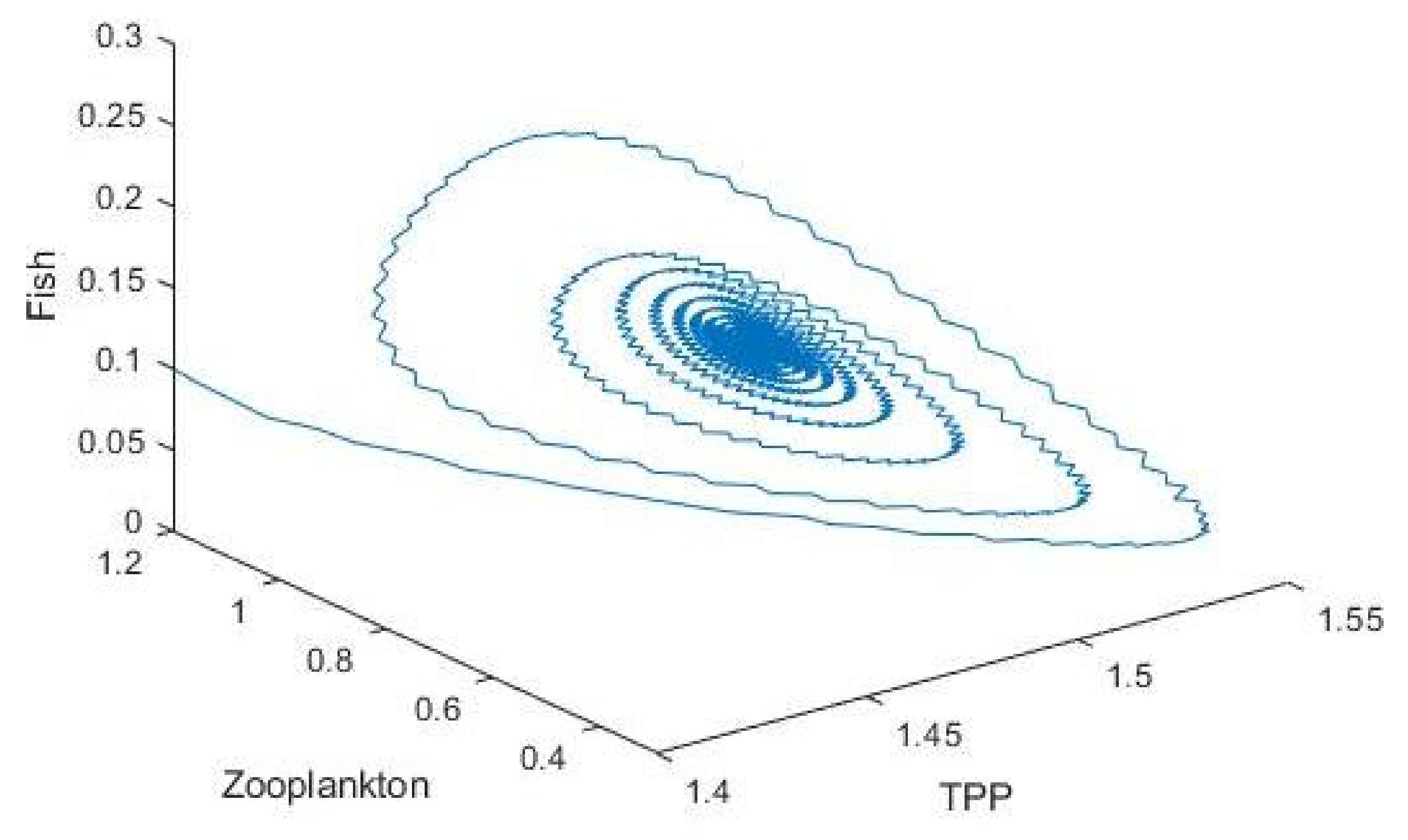
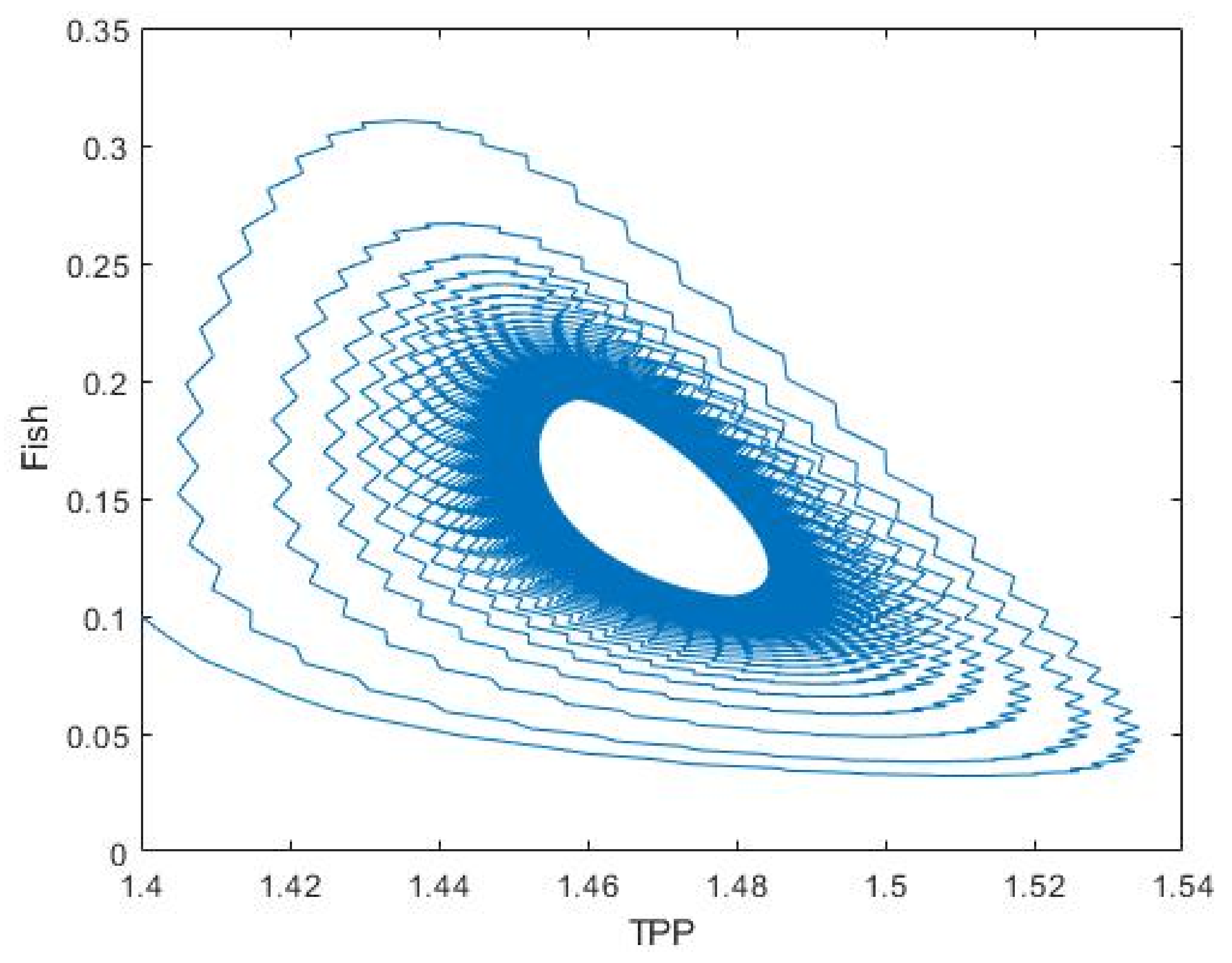
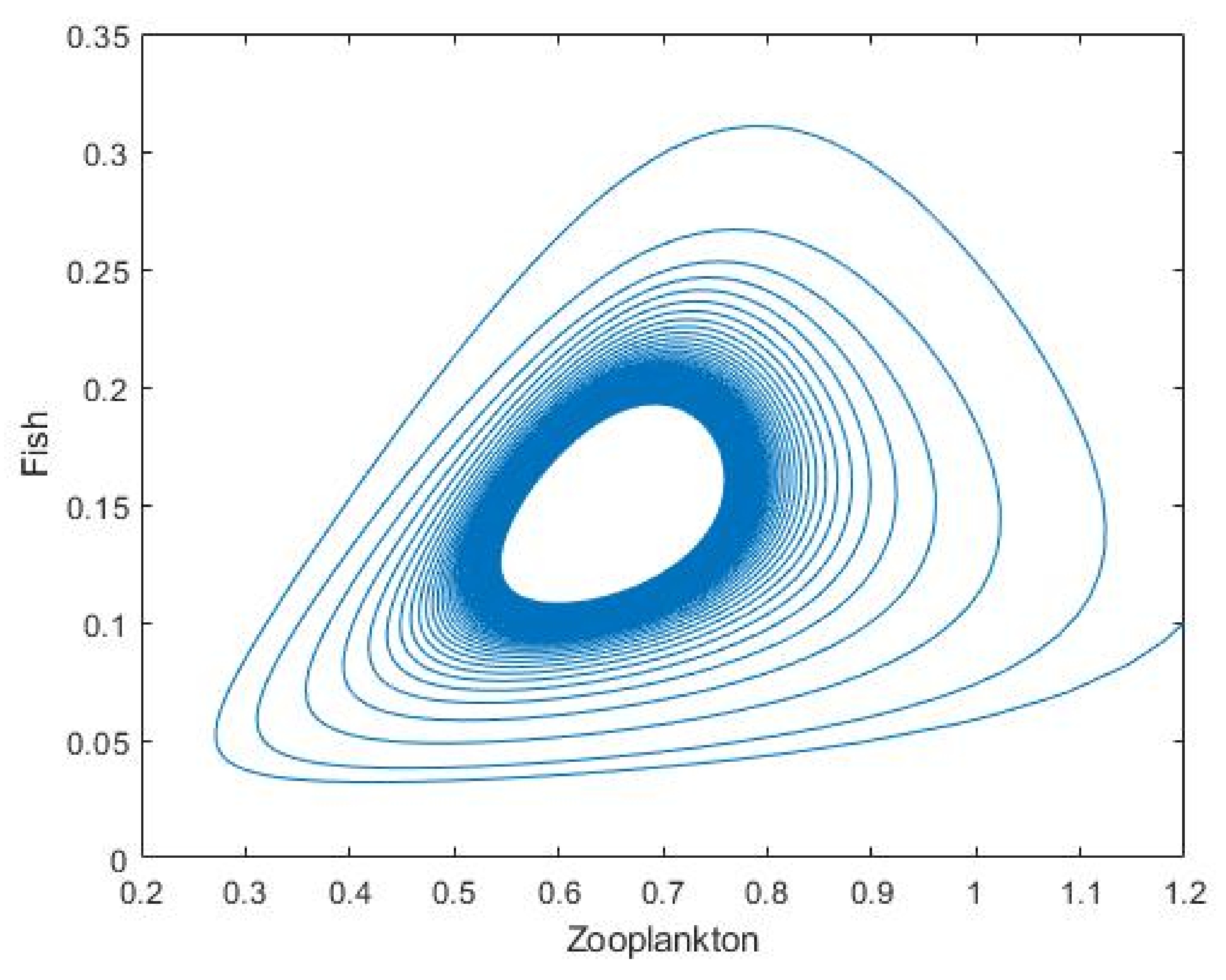
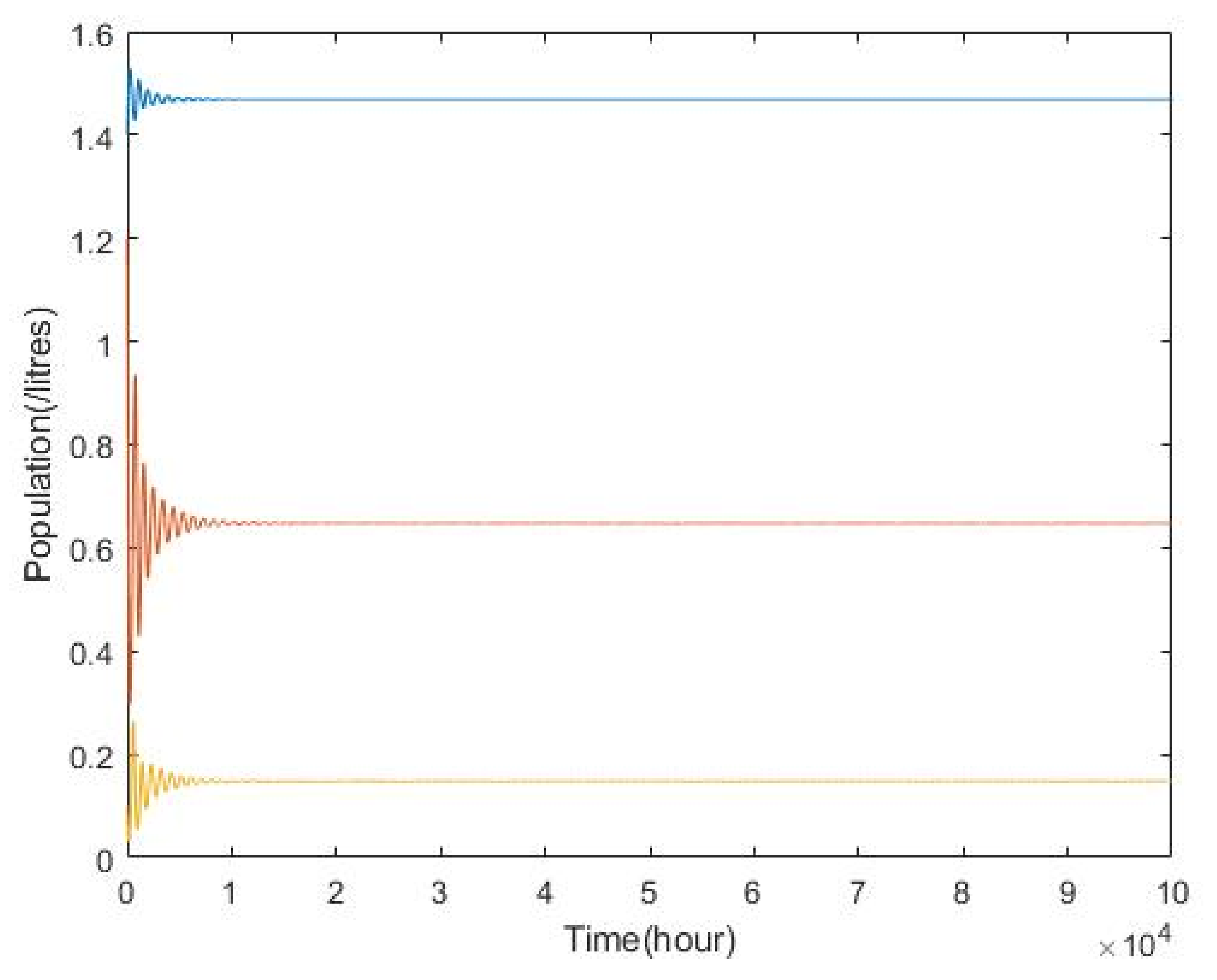
2.2. Plankton–Zooplankton–Fish Interaction Model

This model describes the effects of HABs on fish populations by providing knowledge and understanding on how the fish could die. A delay term is incorporated into the model to show that the mortality of the fish populations is not an instantaneous process. The developed model is as follows:

$$\begin{array}{cc}\hfill \frac{dx}{dt}& =rx\left(t\right)(1-x\left(t\right)/K)-c_{1}x\left(t\right)y\left(t\right)\hfill \\ \hfill \frac{dy}{dt}& =e_1{c}_{1}x\left(t\right)y\left(t\right)-c_{2}y\left(t\right)z\left(t\right)-d_{1}y\left(t\right)\hfill \\ \hfill \frac{dz}{dt}& =e_2{c}_{2}y\left(t\right)z\left(t\right)-d_{2}z\left(t\right)-fy\left(t\right)z(t-\tau )\hfill \end{array}$$

(16)

The following set of assumptions is assumed to formulate the fish mathematical model:

• Let $x\left(t\right)$ be the toxin production phytoplankton (TPP) which are being consumed by the zooplankton population which in turn serves as food for the fish population, $f\left(t\right)$.
• Let r be the intrinsic growth rate of phytoplankton; K be the environmental capacity of phytoplankton; and $c_1$ be the predation rate of zooplankton while $c_2$ is the predation rate of fish.
• $e_1$ is the birth rate of zooplankton while $e_2$ is the birth rate of fish, $d_1$ is the mortality rate of zooplankton and $d_2$ is mortality rate of fish, and f is coefficient of toxin substance from TPP.
• Let $\tau$ be the time delay for the fish to die when feeding on the infected zooplankton as this is not an instantaneous process. The infected zooplankton become harmful to the fish when eaten.

$$J=\left[\begin{array}{ccc}-c_{1}y-\frac{r(2x-K)}{K}& -c_{1}x& 0\\ e_1{c}_{1}y& e_1{c}_{1}x-c_{2}z-d_1& -c_{2}y\\ 0& e_2{c}_{2}z-fz& e_2{c}_{2}y-d_2\end{array}\right],$$

(17)

where

$$\begin{array}{cc}\hfill H_1& =-\frac{rx}{K}+r(1-\frac{x}{K})-c_{1}y\hfill \\ \hfill H_2& =-d_1+c_1{e}_{1}x-c_{2}z\hfill \\ \hfill H_3& =c_2{e}_{2}y-d_2\hfill \end{array}$$

(18)

$$N=\left[\begin{array}{ccc}0& 0& 0\\ 0& 0& 0\\ 0& 0& -fy\end{array}\right]$$

(19)

The characteristic equation is

$$\begin{array}{c}\hfill F(\lambda ,\tau )={\lambda }^3+A_1{\lambda }^2+A_2\lambda +A_3+(B_1{\lambda }^2+B_2\lambda +B_3)e^{-\lambda \tau }\end{array}$$

(20)

where

$A_1=-H_1-H_2-H_3$

$A_2=H_1{H}_2+H_1{H}_3+H_2{H}_3+c_1^2{e}_{1}xy+c_2^2{e}_{2}yz$

$A_3=-H_1{H}_2{H}_3-c_1^2{e}_1{H}_{3}xy-c_2^2{e}_2{H}_{1}yz$

$B_1=fx$

$B_2=-f{H}_{1}x-f{H}_{2}x$

$B_3=fx{H}_1{H}_2+C_1^2{e}_{1}f{x}^{2}y+c_1{c}_{2}fxyz$

substitute $\lambda =iw$ into Equation (20)

$$\begin{array}{c}{\left(iw\right)}^3+A_1{\left(iw\right)}^2+A_2\left(iw\right)+A_3+(B_1{\left(iw\right)}^2+B_2\left(iw\right)+B_3)e^{-}iw\tau =0\\ -i{w}^3-A_1{w}^2+A_{2}iw+A_3+(-B_1{w}^2+B_{2}iw+B_3)(cosw\tau +isinw\tau )=0\\ -i{w}^3-A_1{w}^2+i{A}_{2}w+A_3+(-B_1{w}^{2}cosw\tau -i{B}_1{w}^{2}sinw\tau +B_{2}iwcosw\tau -B_{2}wsinw\tau +\\ B_{3}cosw\tau +i{B}_{3}sinw\tau =0\end{array}$$

(21)

separate imaginary and real parts

$$\begin{array}{c}\hfill I:-w^3+A_{2}w-B_1{w}^{2}sinw\tau +B_{2}wcosw\tau +B_{3}sinw\tau \\ \hfill R:-A_1{w}^2+A_3-B_1{w}^{2}cosw\tau -B_{2}wsinw\tau +B_{3}cosw\tau \end{array}$$

(22)

$$\begin{array}{c}\hfill -w^3+A_{2}w=B_1{w}^{2}sinw\tau -B_{2}wcosw\tau -B_{3}sinw\tau \\ \hfill -A_1{w}^2+A_3=B_1{w}^{2}cosw\tau +B_{2}wsinw\tau -B_{3}cosw\tau \end{array}$$

(23)

square and add up the equations

$w^6+(A_1^2-2A_2-B_1^2+2B_1{B}_2)w^4+(A_2^2-2A_1{A}_3+2B_1{B}_3+B_2^2)w^2+A_3^2-B_3^2=0$ where

$$\begin{array}{cc}\hfill C_1& =A_1^2-2A_2-B_1^2+2B_1{B}_2\hfill \\ \hfill C_2& =A_2^2-2A_1{A}_3+2B_1{B}_3+B_2^2\hfill \\ \hfill C_3& =A_3^2-B_3^2\hfill \end{array}$$

(24)

let $u=w^2$

$$u^3+C_1{u}^2+C_{2}u+C_3=0$$

(25)

then $H^{\prime }\left(u\right)=3u^2+2C_{1}u+C_2$

Hence, $H^{\prime }\left(u\right)=0$ has two roots which are given by

$$\begin{array}{c}{u}_1^{*}=\frac{-C_1+\sqrt{(C_1^2-3C_2)]}}{3}\\ u_2^{*}=\frac{-C_1-\sqrt{(C_1^2-3C_2)]}}{3}\end{array}$$

A hypothesis is formulated as below:

Hypothesis 1 (H1).

$u_1^{*}>0,H\left(u_1^{*}\right)<0,C_1^2-3C_2\ge 0$.

Since $C_3>0$, Equation (24) has no real positive roots if $C_1^2-3C_2<0$ (see Lemma 2.1 in [19]) and two real positive roots if Hypothesis 1 (H1) holds and these roots be ${\omega }_j$ (j = 1,2). Let ${\omega }_1<{\omega }_2$ and then $H^{\prime }\left({\omega }_1\right)$ < 0 and $H^{\prime }\left({\omega }_2\right)$ > 0 (see Lemma 3.2 in [20]).

By Equation (23), we obtained following equation

$$sinw\tau =\frac{-A_1{w}^2+A_3+(-B_1{w}^2+B_3)cosw\tau }{B_{2}w}$$

(26)

and substitute it into Equation (23).

$-w^3+A_{2}w=B_1{w}^2\left[\frac{-A_1{w}^2+A_3+(-B_1{w}^2+B_3)cosw\tau }{B_{2}w}\right]-B_{2}wcosw\tau -\left[\frac{-A_1{w}^2+A_3+(B_3-B_1{w}^2)cosw\tau }{B_{2}w}\right]$

$$\begin{array}{c}\hfill cosw\tau =\frac{-B_2{w}^4+B_2{A}_2{w}^2+A_1{B}_1{w}^4-A_3{B}_1{w}^2-A_1{B}_3{w}^2+A_3{B}_3}{B_1{B}_3-B_1^2{w}^4-B_2^2{w}^2-B_3^2+B_1{B}_3{w}^2}\\ \hfill {\tau }_j^k=\frac{1}{w_j}\left[arccos\left(\frac{-B_2{w}^4+B_2{A}_2{w}^2+A_1{B}_1{w}^4-A_3{B}_1{w}^2-A_1{B}_3{w}^2+A_3{B}_3}{B_1{B}_3-B_1^2{w}^4-B_2^2{w}^2-B_3^2+B_1{B}_3{w}^2}\right)+2k\pi \right]\end{array}$$

(27)

where $j=1,2$ and $k=0,1,2,..$

Lemma 1.

If Hypothesis (H1) holds, then Equation (20) has a pair of pure imaginary roots $\mp iw$ and all other roots have non-zero real parts at $\tau ={\tau }_j^k$ (j = 1,2,k = 0,1,2,…)

In addition, we define ${\tau }_0=minj=1,2{\tau }_j^0$, ${\tau }_0$ represents the smallest positive value of ${\tau }_j^0,j=1,2$ given by Equation (26) and $w=w_{j}0$.

Lemma 2.

If Hypothesis (H1) holds, then we have the following two transversality conditions:

$$sign{\left[\frac{dR\lambda \left(\tau \right)}{d\tau }\right]}_{\tau }={\tau }_1^k<0,sign{\left[\frac{dR\lambda \left(\tau \right)}{d\tau }\right]}_{\tau }={\tau }_1^k>0$$

(28)

where $k=0,1,2,\dots$

Therefore, the required transversality condition is obtained if $H^{\prime }\left({\omega }_1^2\right)<0$, and $H^{\prime }\left({\omega }_2^2\right)>0$.

3. Results

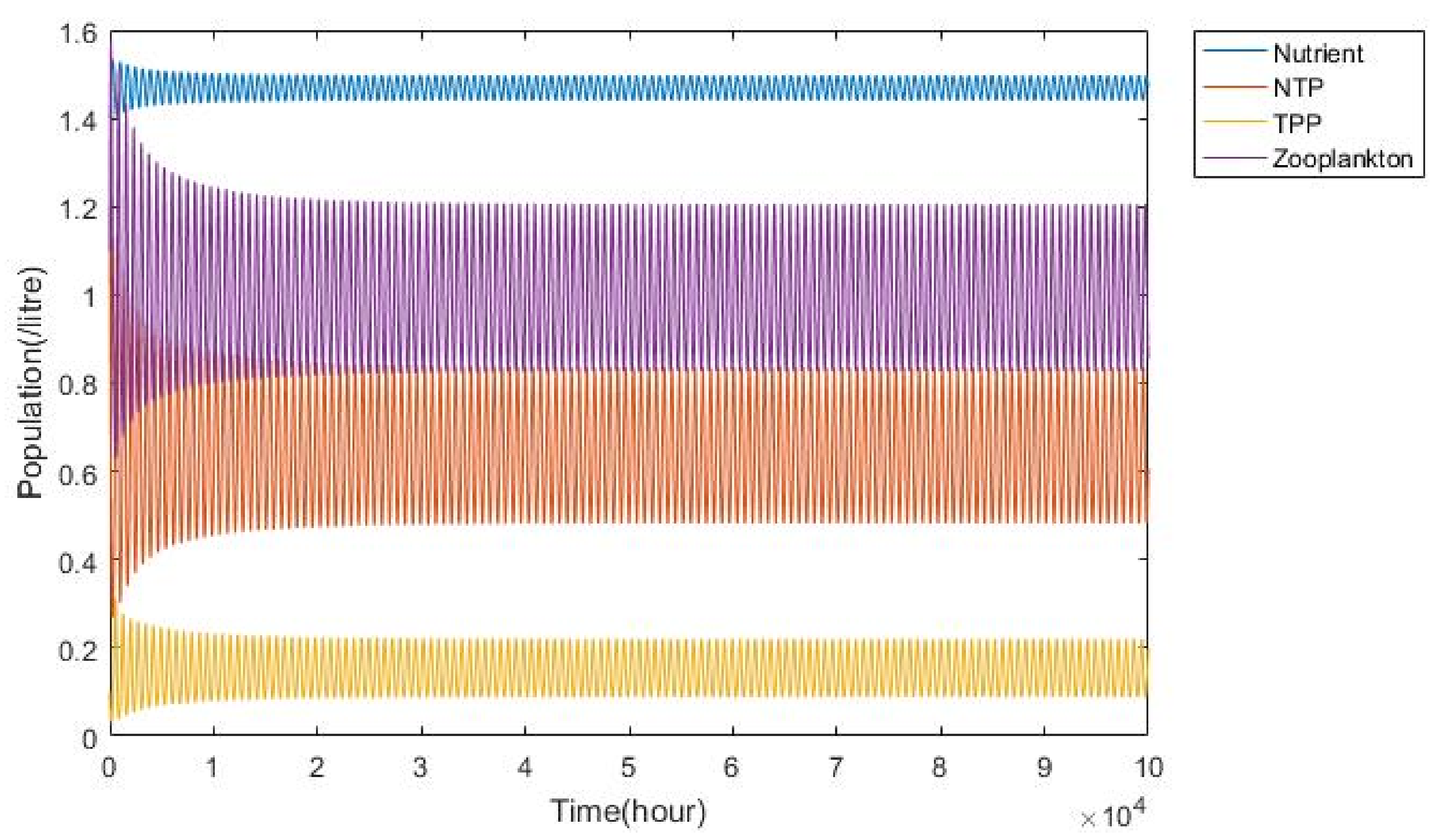
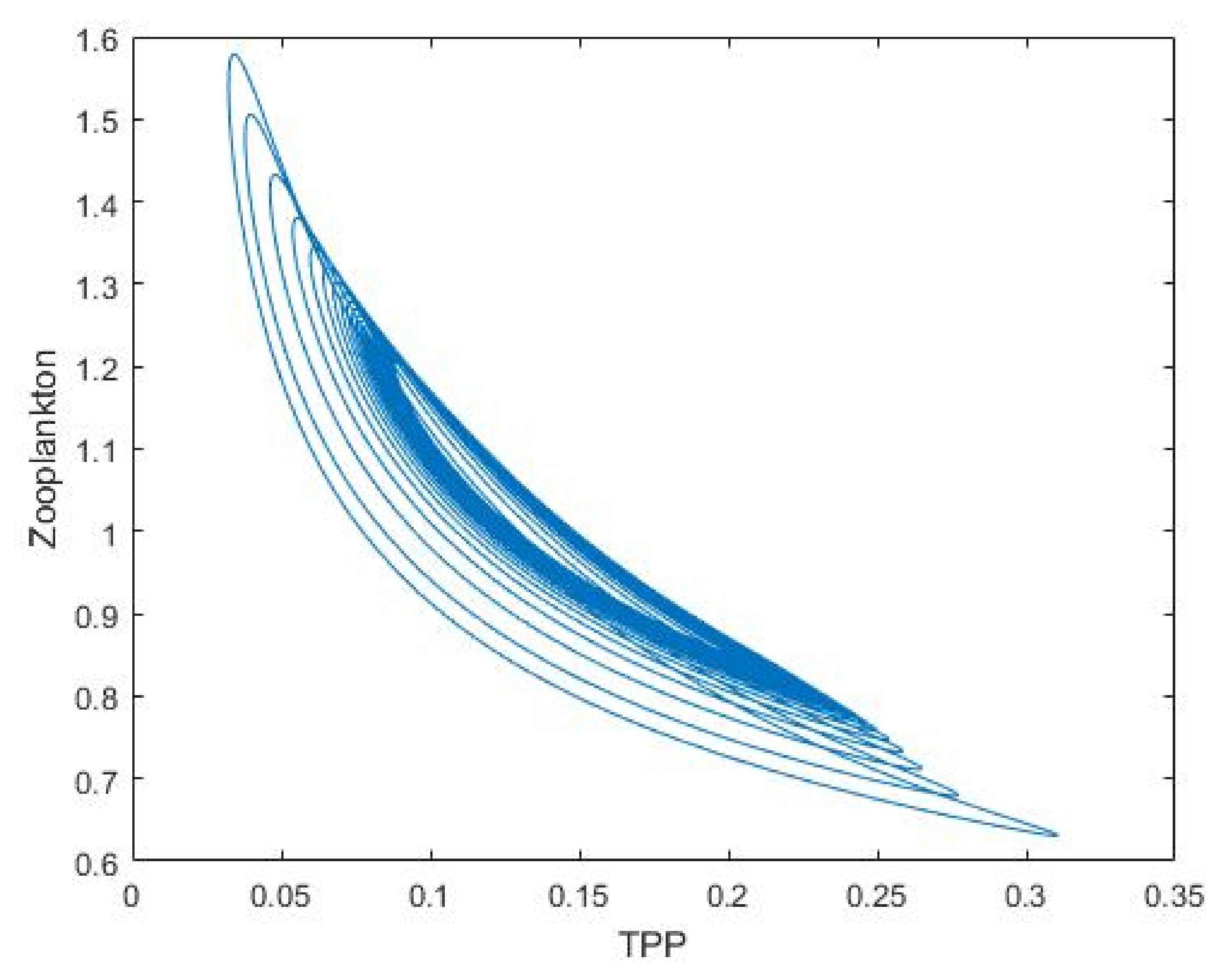
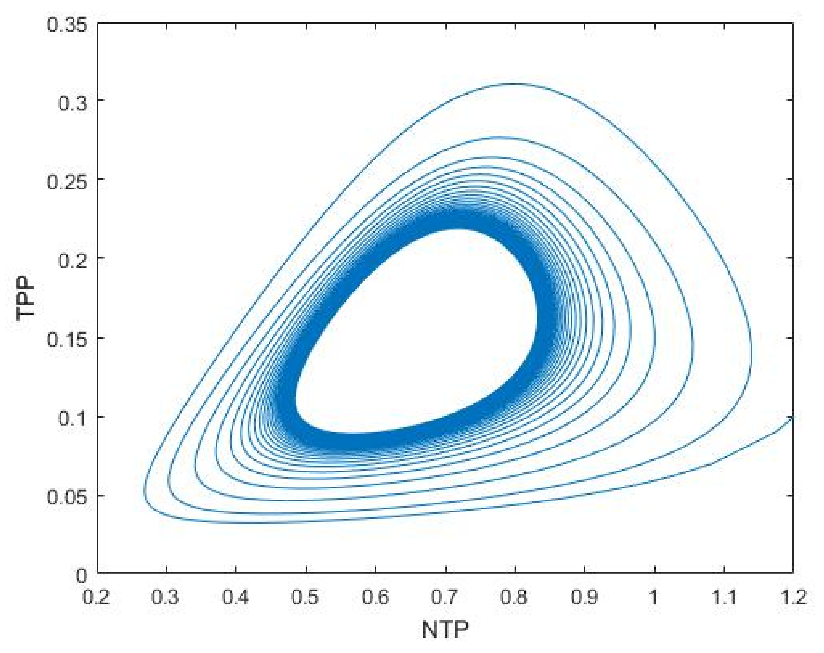
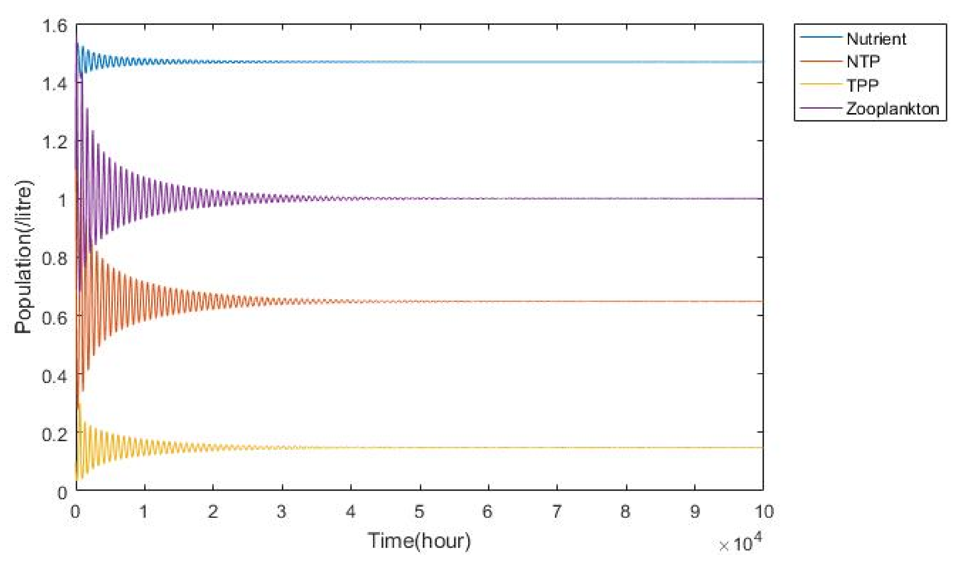
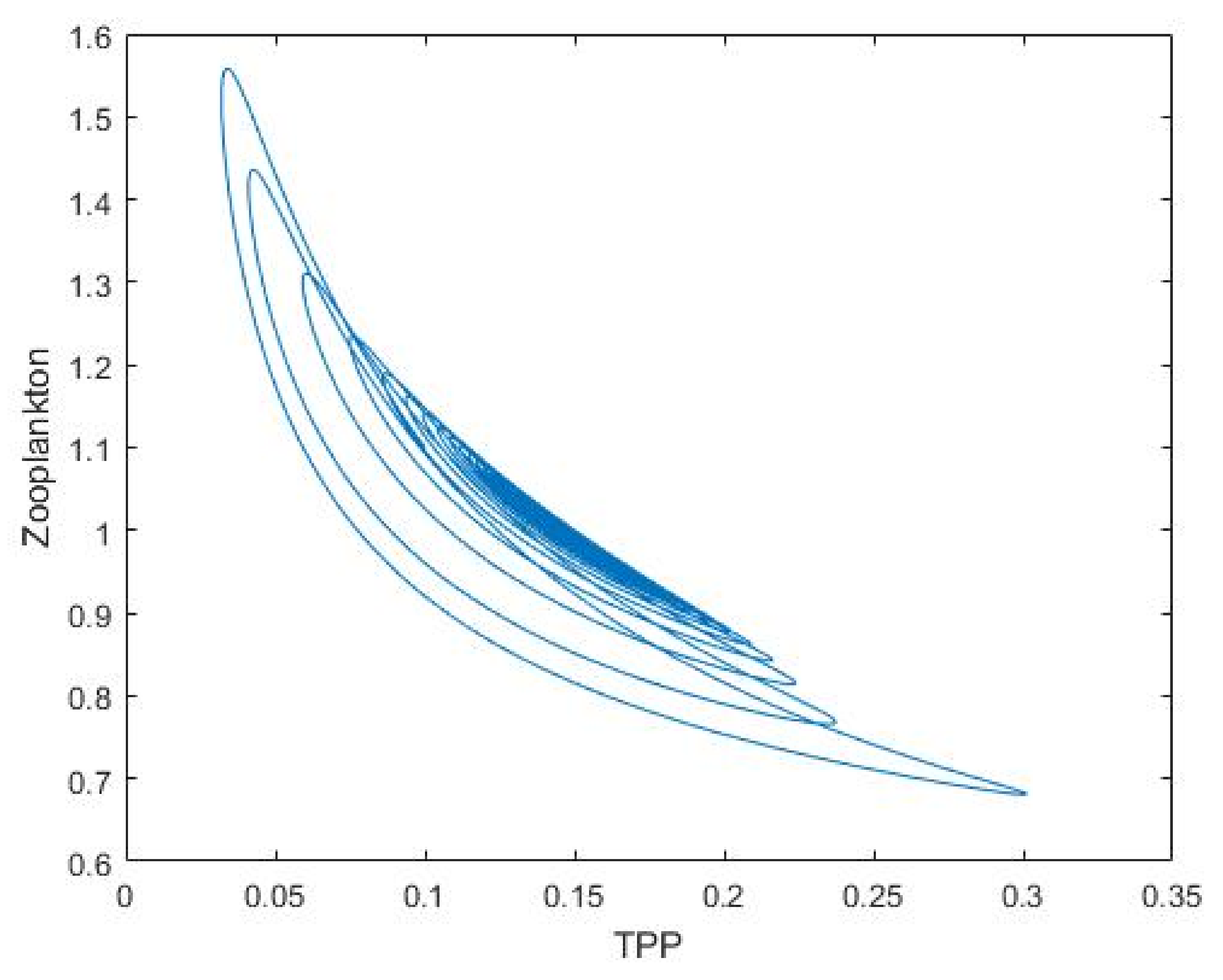
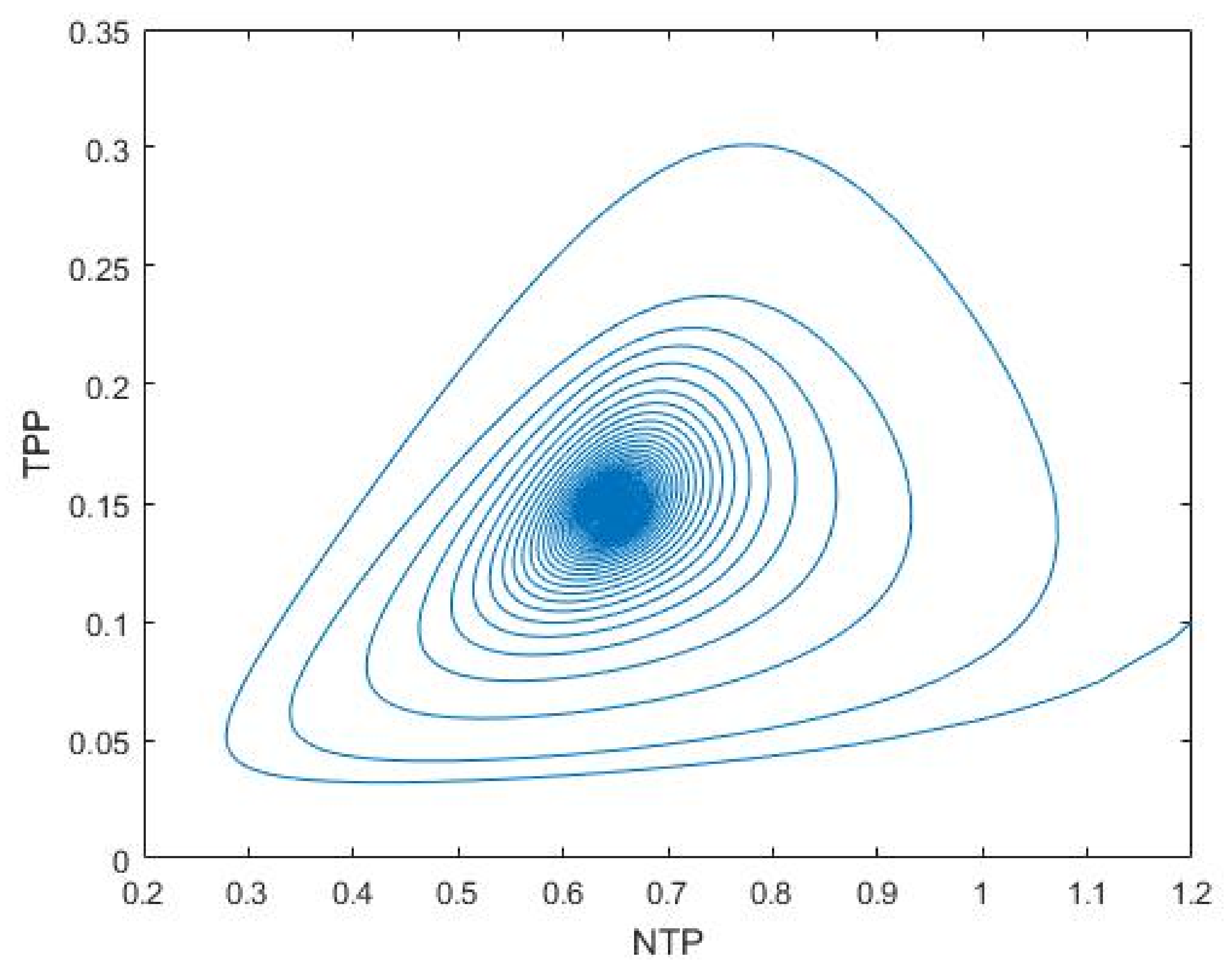
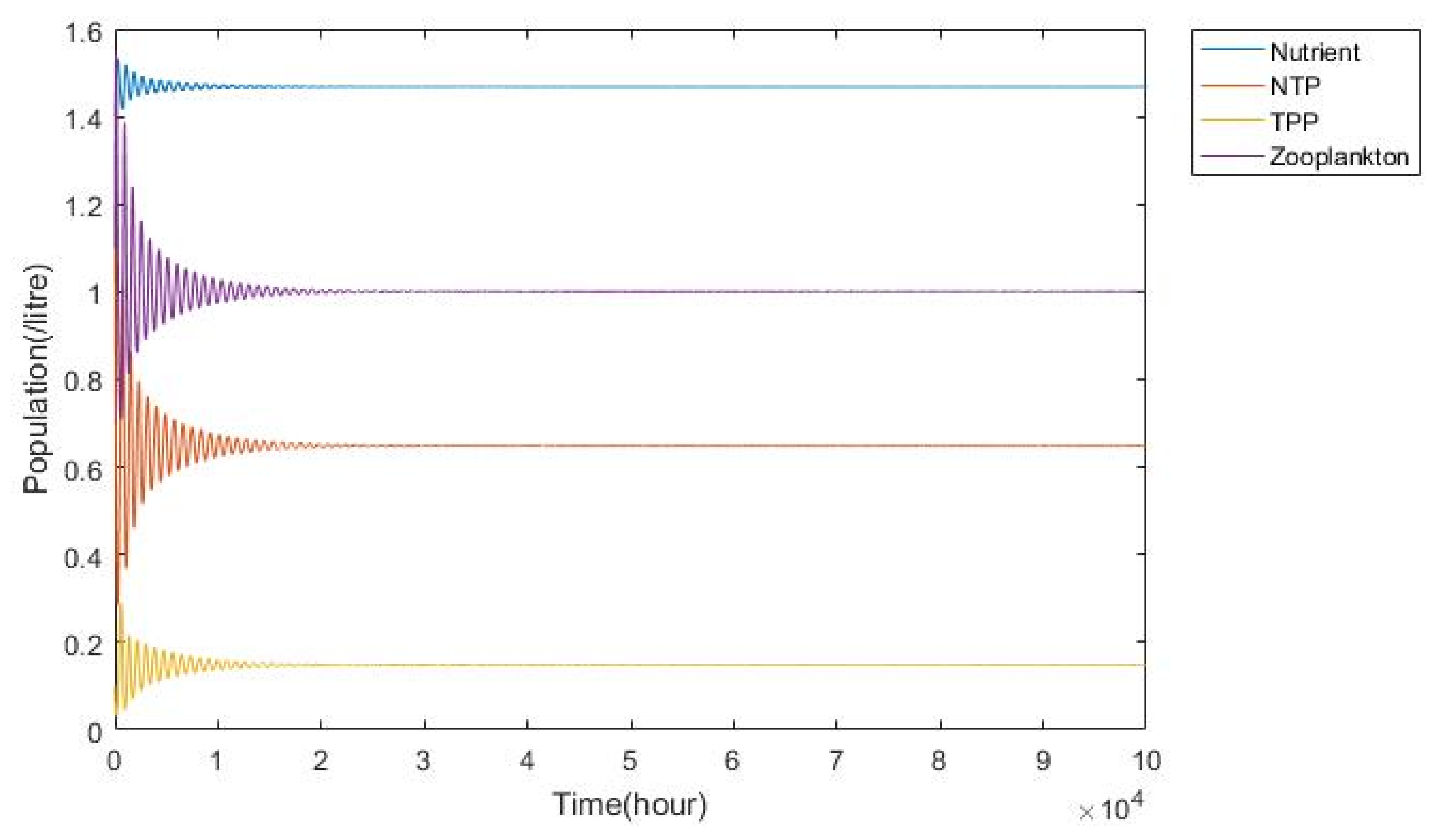
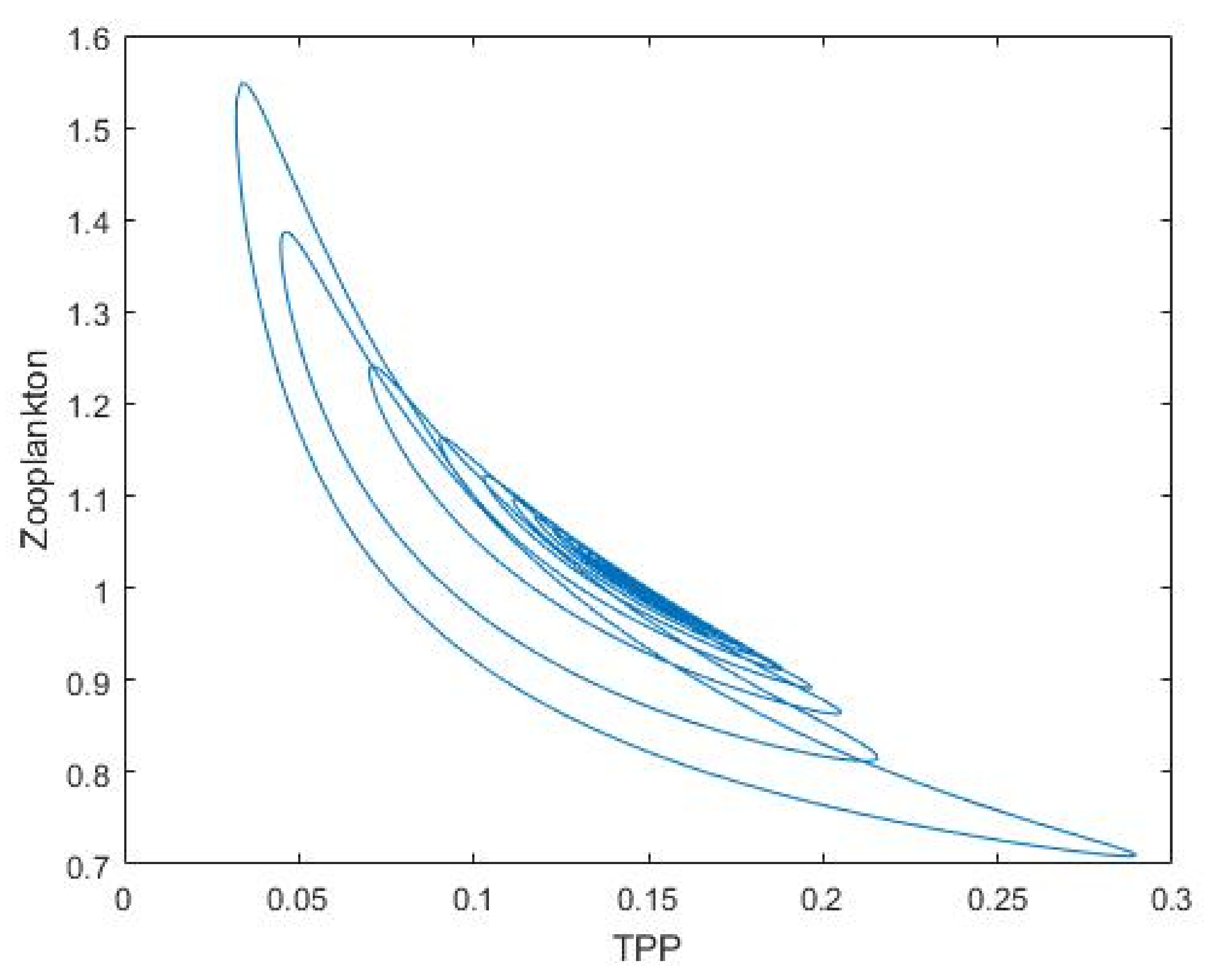
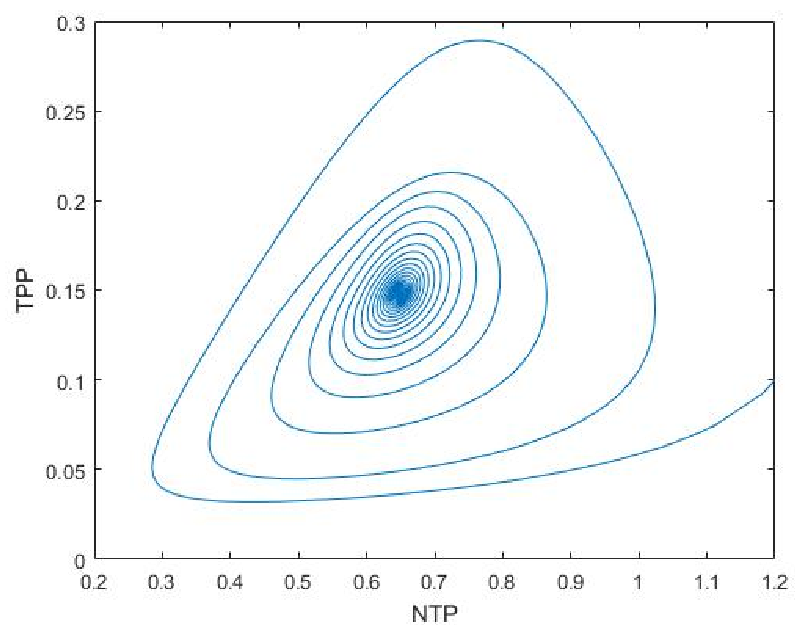
3.1. Nutrient–Phytoplankton–Zooplankton Interaction Model

A set of parameter values from the literature [17] was used to substantiate the analytical results obtained through numerical simulation (see

Table 1. Parameter values used in the numerical simulation (Nutrient–Phytoplankton–Zooplankton Interaction Model).

Parameters	Symbols	Values
Dilution rate of nutrient	D	0.3 (h${}^{-1}$)
Constant input of nutrient concentration	$N_0$	1.58 (h${}^{-1}$)
Nutrient uptake rate for the NTP	${\alpha }_1$	0.03 (mL · h${}^{-1}$)
Nutrient uptake rate for the TPP	${\alpha }_2$	0.022 (mL·h${}^{-1}$)
Conversion rate of NTP	${\theta }_1$	0.02 (mL·h${}^{-1}$)
Conversion rate of TPP	${\theta }_2$	0.02 (mL·h${}^{-1}$)
Natural death rate of NTP	$m_1$	0.006 (h${}^{-1}$)
Natural death rate of TPP	$m_2$	0.006 (h${}^{-1}$)
Natural death rate of zooplankton	$m_3$	0.005 (h${}^{-1}$)
Competition coefficient	$e_1$	0.02 (mL·h${}^{-1}$)
Competition coefficient	$e_2$	0.02 (mL·h${}^{-1}$)
Predation rate of NTP	${\beta }_1$	0.02 (mL·h${}^{-1}$)
Predation rate of TPP	${\beta }_2$	0.01 (mL·h${}^{-1}$)
Conversion rate for NTP	${\gamma }_1$	0.01 (mL·h${}^{-1}$)
Death rate due to consumption of TPP	${\gamma }_2$	0.008 (mL·h${}^{-1}$)
Dilution rate of NTP	$D_1$	0.0004 (h${}^{-1}$)
Dilution rate of TPP	$D_2$	0.0004 (h${}^{-1}$)
Dilution rate of zooplankton	$D_3$	0.0003 (h${}^{-1}$)

). $\tau$ is considered a bifurcation parameter.

From the numerical simulations, it was found that, for $E^{*}(1.4653,0.6618,0.1647,0.9806)$, the system is unstable for $\tau =0$, which is without delay as in Figure 1. The assumption for the system without delay means that the produced toxin is an instantaneous process neglecting the maturity of the TPP population. Therefore, the absence of time lag in the system illustrates that HAB phenomena will occur faster and thus makes the system unstable. Figure 2 depicts the equilibrium between TPP and zooplankton populations loses its stability for $\tau =0<{\tau }_0$. This shows that an prey–predator interaction exists between TPP and zooplankton population. TPP do not secrete out the toxic substance into the environment but it will harm zooplankton if it is consumed when the toxin produced is at its peak. Meanwhile, Figure 3 shows that the equilibrium between NTP and TPP populations loses its stability for the non-delay system. The NTP and TPP populations interact during the interspecies competition for food hunting.

From the analytical findings, the value of the delay parameter of system (2) for the stability behaviour changes when ${\tau }_0=22.6841$. This finding is well supported by experimental research [3,11] where, in the batch culture of Pyrodinium bahamense in one month, the peak of the cell content is on the 22nd day. The toxin content rapidly peaks during the early exponential phase and rapidly declines prior to the onset of the plateau phase. This explains the reason behind the switching behaviour which occurred once in this research. We also remark that $\tau$ represents the time lag for the maturity of the TPP population for producing toxin.

Therefore, as $\tau$ passes through the critical value of $\tau ={\tau }_0=22.6841$, the interior equilibrium point gains its stability and a Hopf bifurcation occurs as shown in Figure 4. It can be seen that the system switches from an unstable to stable system. Due to the time needed for the maturity of the TPP population, the system becomes locally stable since the HAB takes time to occur. Figure 5 and Figure 6 illustrate the asymptotical stability of the equilibrium between the TPP with the zooplankton population and the NTP with the TPP populations, respectively. It was found that a stable Hopf-bifurcating periodic solution occurred in both figures.

Then, the interior equilibrium point remains locally asymptotically stable whenever the value of $\tau =30>{\tau }_0$ increases, as shown in Figure 7. It can be seen that when the value $\tau$ is longer than ${\tau }_0$, the unstable system becomes stable. A longer time lag describes that the TPP needs a longer time to mature and liberate toxic chemicals. Hence, the system becomes stable where, in this context, the HAB does not occur during the time lag because no toxic chemicals are released that could harm the marine ecosystem. Figure 8 and Figure 9 depict the asymptotical stability of the equilibrium between TPP with the zooplankton populations and NTP with TPP populations for the solution of system (2) for $\tau =30>{\tau }_0$.

Figure 10 illustrates the simulation results of system (2) with $\tau =20<{\tau }_0$. The periodic solution occurs and the interior equilibrium point loses its stability as $\tau$ has a smaller value than the critical value ${\tau }_0$. The time lag in this model represents the time taken for the TPP population to mature and produce toxin. Therefore, a shorter time lag results in an unstable system because TPP takes a shorter time to mature enough to produce toxin. This will promote the HAB to occur. Figure 11 and Figure 12 show that the equilibrium loses its stability between TPP with zooplankton and NTP with TPP for $\tau <{\tau }_0$.

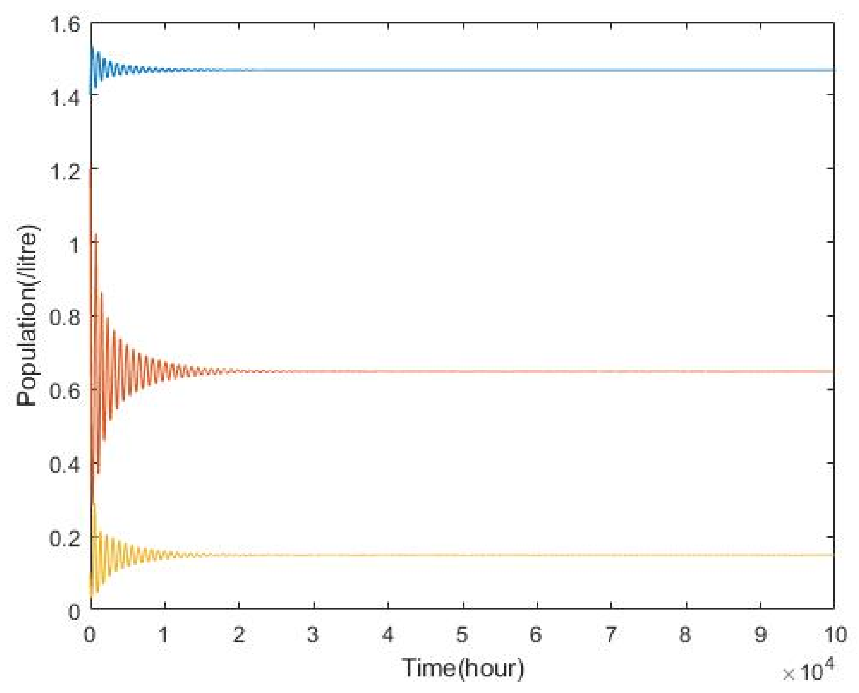
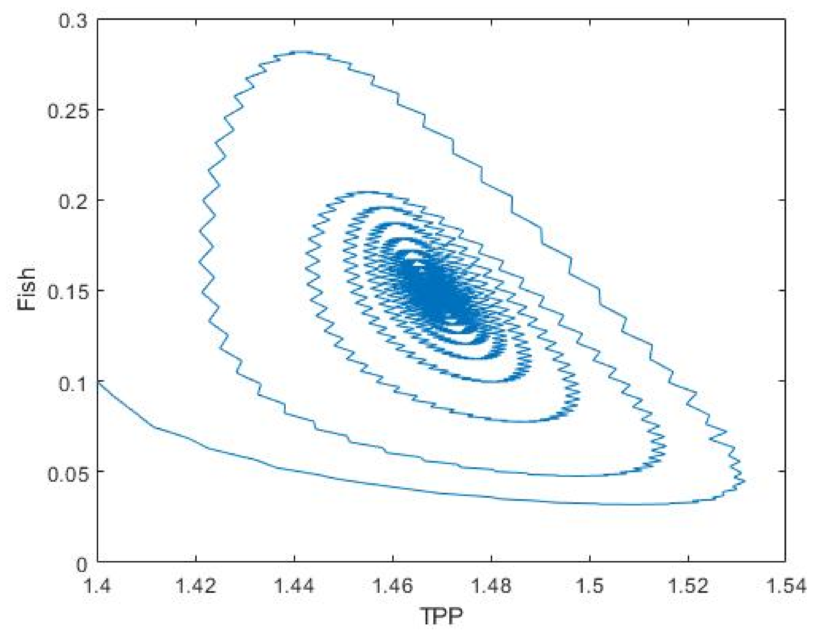
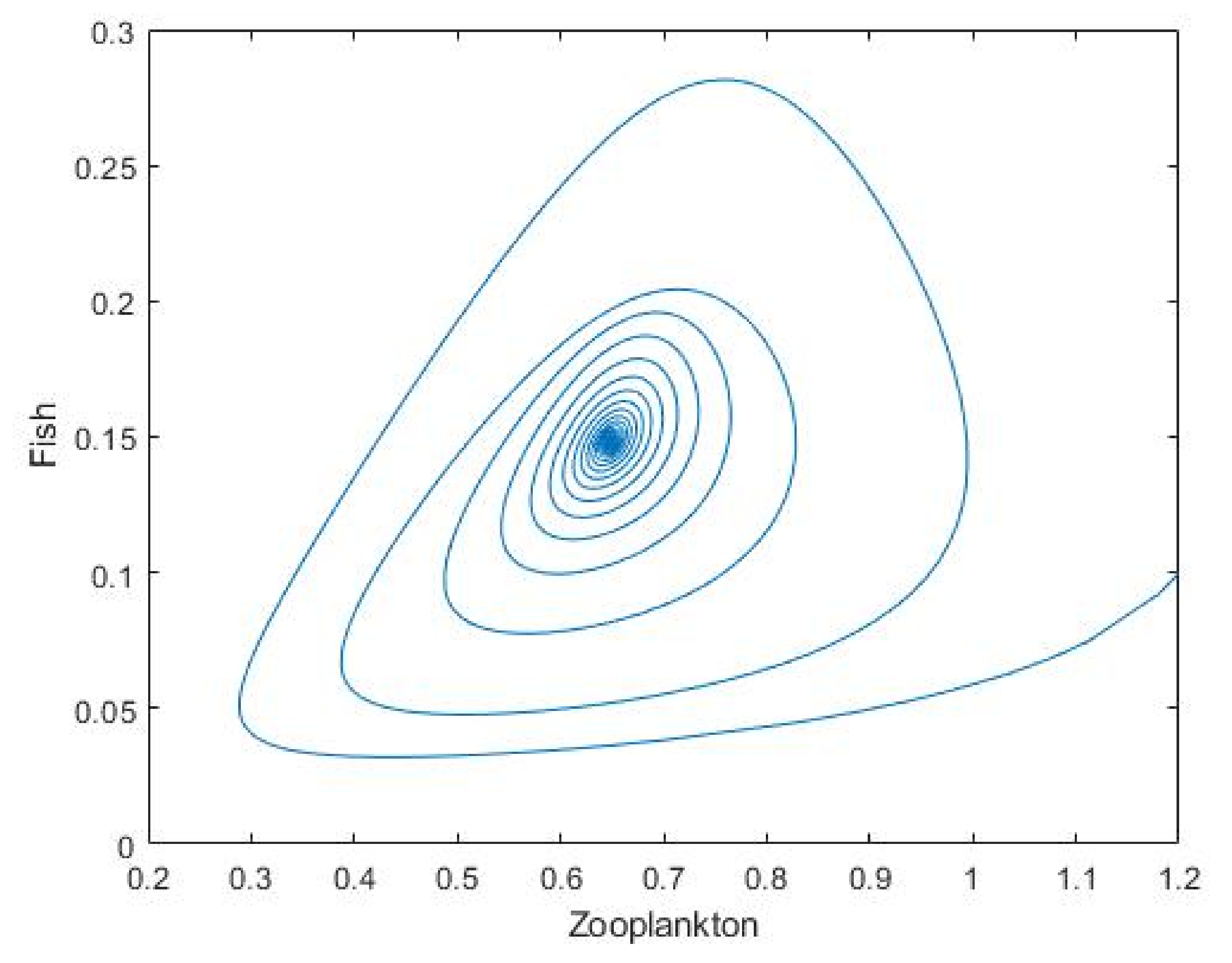
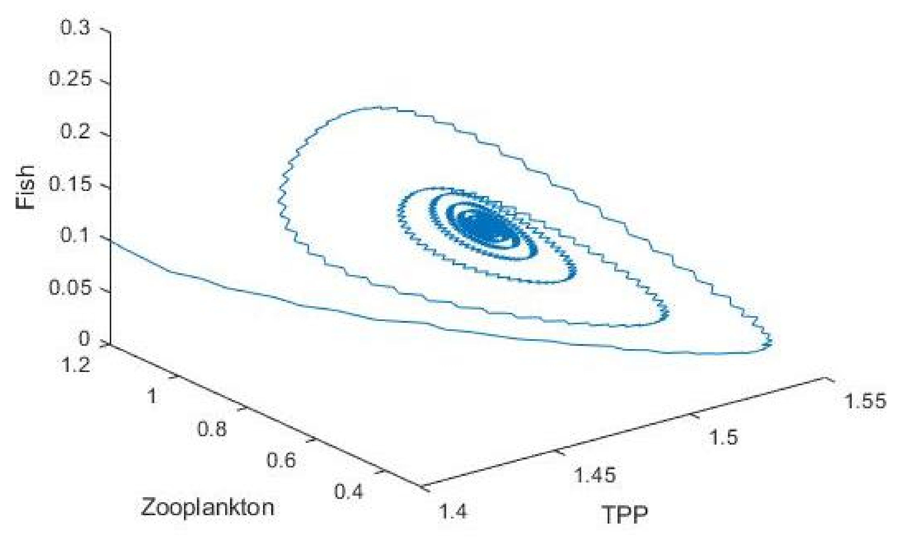
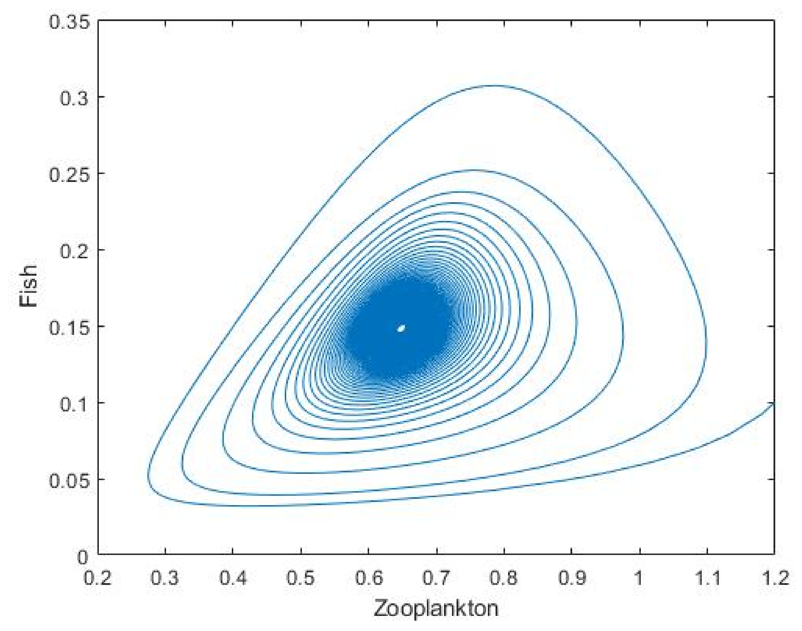
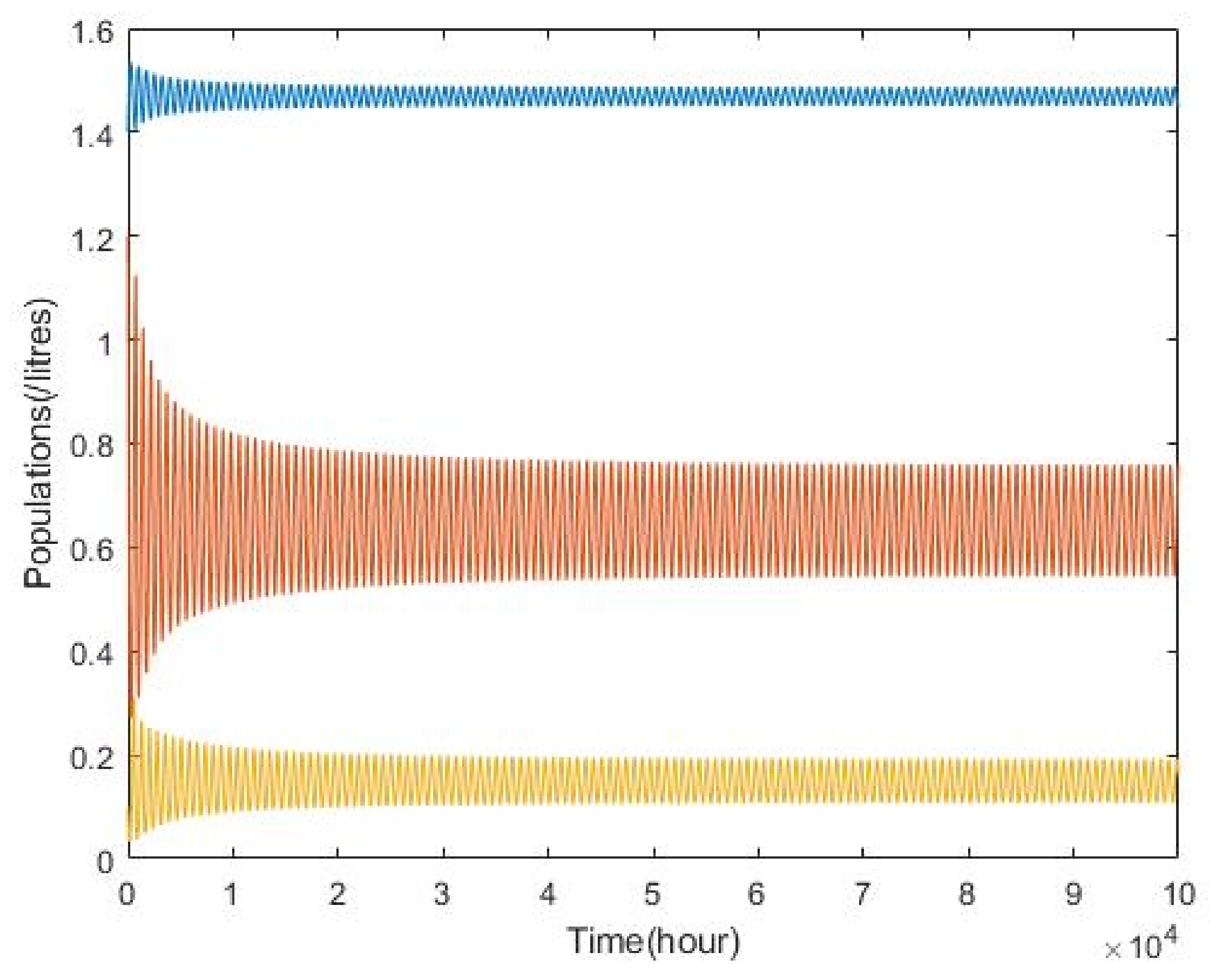
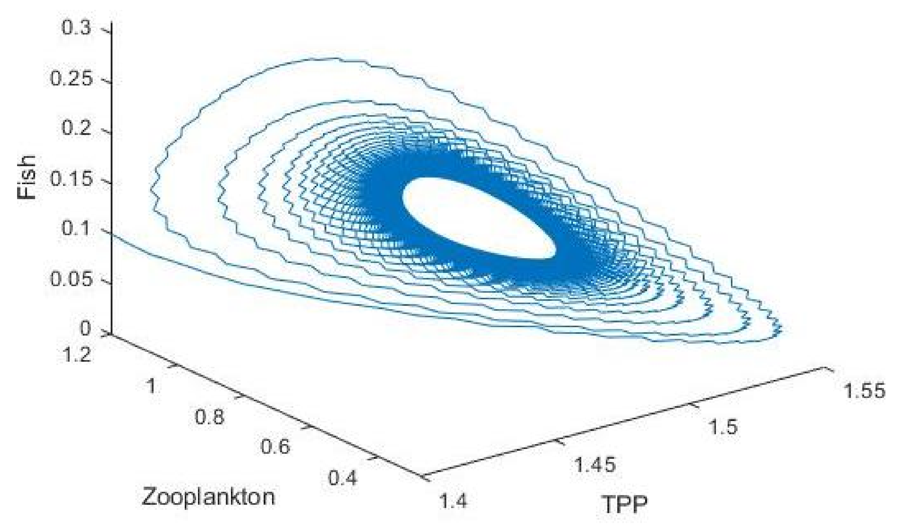
3.2. Plankton–Zooplankton–Fish Interaction Model

From the numerical simulations, it was found that, for $E^{*}(6.6731,3.36538,3.51923)$, the system is stable for $\tau =0$, which means that there is no delay as in Figure 13. The parameter values used in the numerical simulation are as shown in

Table 2. Parameter values used in the numerical simulation (Plankton–Zooplankton–Fish Interaction Model).

Parameters	Symbols	Values
Intrinsic growth rate	r	0.7 (mL·h${}^{-1}$)
Constant input of nutrient concentration	K	28 (h${}^{-1}$)
Mortality rate of zooplankton	$d_1$	0.23 (h${}^{-1}$)
Mortality rate of fish	$d_2$	0.15 (h${}^{-1}$)
Predation rate of zooplankton	$c_1$	0.65 (mL·h${}^{-1}$)
Predation rate of fish	$c_2$	0.45 (mL·h${}^{-1}$)
Birth rate of zooplankton	$e_1$	0.9 (mL·h${}^{-1}$)
Birth rate of fish	$e_2$	0.99 (mL·h${}^{-1}$)
Coefficient of toxicity	f	0.1 (h${}^{-1}$)

.

The asymptotical stability between TPP with fish, zooplankton with fish and among all populations for $\tau =0$ is as shown in Figure 14, Figure 15 and Figure 16. When the system is described as stable it means that fish kills occur in the water while the system is unstable when there no fish kills occur. This is because the objective of this model is to describe the fish kills due to HAB events. Meanwhile, the delay in this model indicates the time lag required for the fish to die after consuming the toxicated zooplankton. The values of $\tau$ are as in

Table 3. $\tau$ values.

${\mathit{\tau }}_{\mathit{j}}^{+}$	${\mathit{\tau }}_{\mathit{j}}^{-}$
${\tau }_0^{+}=1.37941$	${\tau }_0^{-}=5.39314$
${\tau }_1^{+}=6.98104$	${\tau }_1^{-}=12.53884$
${\tau }_2^{+}=12.58266$	${\tau }_2^{-}=19.6845$

.

From Figure 17, it can be seen that when the value of $\tau ={\tau }_0^{+}=1.37941$, the system becomes periodic and switches from a stable system to an unstable system and Hopf bifurcation occurs. This shows that the induced delay in this system affects the stability of the system. The equilibrium losing its stability between the TPP with fish, zooplankton with fish and among all populations are shown in Figure 18, Figure 19 and Figure 20.

However, Figure 21 illustrates that the system again switches to a stable system when the value of $\tau ={\tau }_0^{-}=5.39314$. Thus, ${\tau }_0^{-}$ is the second bifurcation node in this system where the system changes from an unstable system to a stable system. The asymptotical stability between TPP with fish, zooplankton with fish and among all populations are as shown in Figure 22, Figure 23 and Figure 24.

Meanwhile, Figure 25 shows that the system becomes unstable again when the value of $\tau ={\tau }_1^{+}=6.98104$. Therefore, this is the third bifurcation node in this system where the system switches from being a stable to unstable system. It can be seen that the system oscillates throughout the period. Equilibrium between the TPP with fish, zooplankton with fish and among all populations loses its stability as shown in Figure 26, Figure 27 and Figure 28.

However, the system remains unchanged when $\tau ={\tau }_1^{-}=12.53884$, as shown in Figure 29. Thus, there is no Hopf bifurcation since there is no switching. The equilibrium between TPP with fish, zooplankton with fish and among all populations loses its stability for ${\tau }_1^{-}$ are shown as in Figure 30, Figure 31 and Figure 32.

Figure 33 illustrates the direction of Hopf while Figure 34 shows the stability information of System (16). It can be seen that for $\tau =0$, which is without delay, the system is stable. However, the system switches to an unstable system for the first critical value of time delay which is $\tau ={\tau }_0^{+}=1.37941$. The system is asymptotically stable for $\tau <1.37941$. Then, the system again switches to a stable system for the second critical value of the time delay, $\tau ={\tau }_0^{-}=5.39314$. The system loses its stability when $\tau >5.39314$ which is less than the third critical value $\tau >6.98104$. However, the system remains unstable for $\tau >6.98104$ which is less than the fourth critical value $\tau =12.53884$.

4. Discussion

In this research, the interactions between the nutrient, TPP population, NTP population, and zooplankton population were investigated to describe the occurrence of HAB events. The time delay is incorporated into this system to show that TPP species need to achieve their maturity before producing toxin. From the results, it can be seen that the unstable model becomes stable when delay is induced into the system. Whenever the time delay is equal to the critical value—which is ${\tau }_0=22.6841$—the system achieves its stability. The value obtained is well supported by experimental findings [3,11] where in the batch culture of Pyrodinium bahamense, in a month, on the 22nd day, the toxin content is at its most. The toxin content rapidly peaks during the exponential phase and rapidly decline prior to the onset of a plateau phase.

The toxin released by the TPP population has had many detrimental consequences on marine creature, aquaculture sector, tourism, etc. In this research, the effect of toxin on fish populations is discussed where the interaction between TPP species, zooplankton and fish populations is well described. From the model, fish are affected by the toxin when they consumed toxicated zooplankton, which consumed the TPP population. However, the death of a fish population is not an instantaneous process but is mediated by some time lag. Therefore, delay in incorporated into this model to study the effect of delay into this system.

It can be seen that, for $\tau =0$, which is without delay, the system is stable. However, the system switches to an unstable system for the first critical value of time delay which is $\tau ={\tau }_0^{+}=1.37941$. The system is asymptotically stable for $\tau <1.37941$. Then, the system again switches to a stable system for the second critical value of time delay, $\tau ={\tau }_0^{-}=5.39314$. The system loses back its stability when $\tau >5.39314$ which is less than the third critical value $\tau >6.98104$. However, the system remains unstable for $\tau >6.98104$ but less than the fourth critical value $\tau =12.53884$. Therefore, it can be concluded that there are two nodes of Hopf bifurcation which change the system from a stable system to an unstable system and switch back to a stable system and then remain unchanged. In an ecological sense, these results revealed that under certain parametric conditions, the delay of fish death can bring instability as well as stability in the planktonic food chain.

5. Conclusions

This study presented a mathematical model that describes the process of HAB with the presence of discrete delay. The inclusion of discrete delay is important to show that the production of toxin is not an instantaneous process where TPP species need to achieve their maturity before being able to produce toxin in their body. However, the produced toxin does not secrete out into the environment but is kept inside the cell body. P.bahamense becomes harmful to shellfish because shellfish act as a filter feeder and will filter the water going inside them. Thus, when there is massive bloom of P.bahamense, they get stuck in stomach of shellfish during filtration. The toxin does not harm the shellfish but it is harmful to human health whenever it is consumed. Moreover, when there is massive bloom, the decreased content of dissolved oxygen (DO) in the water kills fish because they can barely breathe to receive oxygen. Dinoflagellates have a rigid cell wall that also contains silica and they have two tiny whip-like structures known as flagellae to propel them through the water. Due to this rigid cell wall, it is hard to break but will accumulate in the fish gills and make it hard to breath. In some cases, when the cell wall touches the fish gills, it could explode and the toxin content released out of the cell. This toxin content is harmful to human health if it is consumed.

A delay model of plankton interaction is developed in which the time lag is incorporated for the maturity of TPP species to produce toxin. The stability behaviour of the system around the feasible steady states was investigated. The findings show that inducing discrete delay into the model has a stabilizing effect on the system. This result contradicts previous research wherein almost all of the previous research claimed that delay would stabilize their model system. Therefore, the delay can switch the system from unstable to stable or vice versa [21]. Our findings bring an ecological significance to the marine ecosystem, that is, if the time taken for the TPP to mature is longer, then the system is stable since no production of toxic chemicals could result from the occurrence of HAB. This research indicates that inducing discrete delay causes a stabilization effect in the system and shows the effect of dilution rate, nutrient concentration, and interspecies competition towards the model. This also demonstrates and gives information about the occurrence of HAB for a better understanding.

Furthermore, this study also presented a model of a plankton–fish–zooplankton interaction model which consist of three variables which are the TPP, zooplankton, and fish populations. In this model, the TPP population is being predated by the zooplankton population which in turn serves as food for the predator fish population. The time delay was incorporated into this model to show that the mortality of fish species due to the consumption of toxic zooplankton is not an instantaneous process but is mediated by some time lag. This model helps to understand and describe the effect of toxin liberation by the TPP population towards fish population where fish will die. This may harm the aquaculture sector where massive fish kills during HAB occurrence have occurred in Tanjung Kupang, Johor [10].

Therefore, this research gives knowledge and understanding of how HAB events occur due to Pyrodinium bahamense sp. and what factors are involved. Additionally, the second model describes the effect of HAB on the fish population in which it causes fish mortality. Hence, monitoring and awareness programs should be conducted to educate the public about the effects of HAB occurrence in order to minimize the loss.

References

1. Daily, S.C. Available online: http://sinchew-i.com (accessed on 23 January 2005).
2. Zingone, A.; Enevoldsen, O.H. The diversity of Harmful algal blooms: A challenge for science and management. Ocean Coast. Manag. 2000, 43, 725–748. [Google Scholar] [CrossRef]
3. Usup, G.; Ahmad, A.; Matsuoka, K.; Lim, P.T.; Leaw, C.P. Biology, ecology and bloom dynamics of the toxic marine dinoflagellate Pyrodinium bahamense. Harmful Algae 2012, 14, 301–312. [Google Scholar] [CrossRef]
4. Roy, R.N. Red tide and outbreak of paralytic shellfish poisoning in Sabah. Med J. Malays. 1977, 31, 247–251. [Google Scholar]
5. Suleiman, M.; Jelip, J.; Rundi, C.; Chua, T.H. Case report: Paralytic shellfish poisoning in Sabah, Malaysia. Am. J. Trop. Med. Hyg. 2017, 97, 1731–1736. [Google Scholar] [CrossRef] [PubMed]
6. Jipanin, S.J.; Muhamad-Shaleh, S.R.; Lim, P.T.; Leaw, C.P.; Mustapha, S. The Monitoring of Harmful Algae Blooms in Sabah, Malaysia. J. Phys. Conf. Ser. 2019, 1358, 012014. [Google Scholar] [CrossRef]
7. Arzul, G.; Seguel, M.; Guzman, L.; Denn, E.E. Comparison of allelopathic properties in threetoxic alexandrium species. J. Exp. Mar. Biol. Ecol. 1999, 232, 285–295. [Google Scholar] [CrossRef]
8. Hallam, T.; Clark, C.; Jordan, G. Effects of toxicants on populations: A qualitative approach. II. First order kinetics. J. Theor. Biol. 1983, 18, 25–37. [Google Scholar] [CrossRef] [PubMed]
9. Chakraborty, K.; Das, K. Modeling and analysis of a two-zooplankton one-phytoplankton system in the presence of toxicity. Appl. Math. Model. 2015, 39, 1241–1265. [Google Scholar] [CrossRef]
10. Teen, L.P.; Pin, L.C.; Gires, U. Harmful algal blooms in Malaysian waters. Sains Malays. 2012, 41, 1509–1515. [Google Scholar]
11. Usup, G.; Ahmad, A.; Ismail, N. Pyrodinium bahamense var. compressum red tides studies in Sabah, Malaysia. In Biology, Epidemiology and Management of Pyrodinium Red Tides. Manila: ICLARM Conference Proceedings; Hallegraeff, G.M., Maclean, J.L., Eds.; ICLARM: Bandar Seri Begawan, Brunei, 1989; pp. 97–110. [Google Scholar]
12. Rehim, M.; Zhang, Z.; Muhammadhaji, A. Mathematical Analysis of a Nutrient–Plankton System with Delay. SpringerPlus 2016, 5, 1055. [Google Scholar] [CrossRef] [PubMed]
13. Rehim, M.; Imran, M. Dynamical analysis of a delay model of phytoplankton-zooplankton interaction. Appl. Math. Model. 2012, 36, 638–647. [Google Scholar] [CrossRef]
14. Ma, Z. Mathematical Modelling and Study of Population Ecology; Anhui Education Publishing House: Hefei, China, 1996. [Google Scholar]
15. Holling, C.S. Some characteristics of simple types of predation and parasitism. Can. Entomol. 1959, 91, 385–398. [Google Scholar] [CrossRef]
16. Das, T.; Mukherjee, R.N.; Chaudhuri, K.S. Harvesting of a prey–predator fishery in the presence of toxicity. Appl. Math. Model. 2009, 33, 2282–2292. [Google Scholar] [CrossRef]
17. Bairagi, N.; Pal, S.; Chatterjee, S.; Chattopadhyay, J. Nutrient, non-toxic phytoplankton, toxic phytoplankton and zooplankton interaction in an open marine system. In Aspects of Mathematical Modelling; Birkhäuser: Basel, Switzerland, 2008; pp. 41–63. [Google Scholar]
18. Holmes, M.J.; Teo, S.L. Toxic marine dinoflagellates in Singapore waters that cause seafood poisonings. Clin. Exp. Pharmacol. Physiol. 2002, 29, 829–836. [Google Scholar] [CrossRef] [PubMed]
19. Ruan, S.; Wei, J. On the zeros of transcendental functions with applications to stability of delay differential equations with two delays. Dyn. Contin. Discret. Impuls. Syst. Ser. A 2003, 10, 863–874. [Google Scholar]
20. Li, M.Y.; Shu, H. Multiple stable periodic oscillations in a mathematical model of CTL response to HTLV-I infection. Bull. Math. Biol. 2011, 73, 1774–1793. [Google Scholar] [CrossRef] [PubMed]
21. Sipahi, R.; Niculescu, S.I.; Abdallah, C.T.; Michiels, W.; Gu, K. Stability and stabilization of systems with time delay. IEEE Control Syst. 2011, 31, 38–65. [Google Scholar]
Figure 1. Simulation results of System (2) with τ = 0 < τ 0 .
Mathematics 10 02836 g001
Figure 2. Equilibrium between the TPP and zooplankton populations loses its stability for τ = 0 < τ 0 .
Mathematics 10 02836 g002
Figure 3. Equilibrium between the NTP and TPP populations loses its stability for τ = 0 < τ 0 .
Mathematics 10 02836 g003
Figure 4. Simulation results of System (2) with τ = τ 0 = 22.6841 .
Mathematics 10 02836 g004
Figure 5. The asymptotical stability of equilibrium the between TPP and zooplankton populations for τ = τ 0 = 22.6841 .
Mathematics 10 02836 g005
Figure 6. The asymptotical stability of the equilibrium between NTP and TPP populations for τ = τ 0 = 22.6841 .
Mathematics 10 02836 g006
Figure 7. Simulation results of System (2) with τ = 30 > τ 0 .
Mathematics 10 02836 g007
Figure 8. The asymptotical stability of the equilibrium between the TPP and zooplankton populations for τ = 30 > τ 0 .
Mathematics 10 02836 g008
Figure 9. The asymptotical stability of the equilibrium between the NTP and TPP populations for τ = 30 > τ 0 .
Mathematics 10 02836 g009
Figure 10. Simulation results of System (2) with τ < τ 0 .
Mathematics 10 02836 g010
Figure 11. Equilibrium between the TPP and zooplankton populations loses its stability for τ < τ 0 .
Mathematics 10 02836 g011
Figure 12. Equilibrium between the NTP and TPP populations loses its stability for τ < τ 0 .
Mathematics 10 02836 g012
Figure 13. Simulation results of System (16) for τ = 0 .
Mathematics 10 02836 g013
Figure 14. The asymptotical stability between the TPP and fish populations for τ = 0 .
Mathematics 10 02836 g014
Figure 15. The asymptotical stability between the zooplankton and fish populations for τ = 0 .
Mathematics 10 02836 g015
Figure 16. The asymptotical stability of all populations for τ = 0 .
Mathematics 10 02836 g016
Figure 17. Simulation results of System (16) for τ = τ 0 + .
Mathematics 10 02836 g017
Figure 18. Equilibrium between the TPP and fish populations loses its stability for τ = τ 0 + .
Mathematics 10 02836 g018
Figure 19. Equilibrium between the zooplankton and fish populations loses its stability for τ = τ 0 + .
Mathematics 10 02836 g019
Figure 20. Equilibrium of all populations loses its stability for τ = τ 0 + .
Mathematics 10 02836 g020
Figure 21. Simulation results of System (16) for τ = τ 0 .
Mathematics 10 02836 g021
Figure 22. The asymptotical stability between the TPP and fish populations for τ = τ 0 .
Mathematics 10 02836 g022
Figure 23. The asymptotical stability between the zooplankton and fish populations for τ = τ 0 .
Mathematics 10 02836 g023
Figure 24. The asymptotical stability of all populations for τ = τ 0 .
Mathematics 10 02836 g024
Figure 25. Simulation results of System (16) for τ = τ 1 + .
Mathematics 10 02836 g025
Figure 26. Equilibrium between the TPP and fish populations loses its stability for τ = τ 1 + .
Mathematics 10 02836 g026
Figure 27. Equilibrium between the zooplankton and fish populations loses its stability for τ = τ 1 + .
Mathematics 10 02836 g027
Figure 28. Equilibrium of all populations loses its stability for τ = τ 1 + .
Mathematics 10 02836 g028
Figure 29. Simulation results of System (16) for τ = τ 1 .
Mathematics 10 02836 g029
Figure 30. Equilibrium between the TPP and fish populations loses its stability for τ = τ 1 .
Mathematics 10 02836 g030
Figure 31. Equilibrium between the zooplankton and fish populations loses its stability for τ = τ 1 .
Mathematics 10 02836 g031
Figure 32. Equilibrium of all populations loses its stability for τ = τ 1 .
Mathematics 10 02836 g032
Figure 33. Direction of Hopf.
Mathematics 10 02836 g033
Figure 34. Stability information of System (16).
Mathematics 10 02836 g034