Predictability of Population Fluctuations

Abstract

Population dynamics is affected by environmental fluctuations (such as climate variations), which have a characteristic correlation time. Strikingly, the time scale of predictability can be larger for the population dynamics than for the underlying environmental fluctuations. Here, we present a general mechanism leading to this increase in predictability. We considered colored environmental fluctuation acting on a population close to equilibrium. In this framework, we derived the temporal auto and cross-correlation functions for the environmental and population fluctuations. We found a general correlation time hierarchy led by the environmental-population correlation time, closely followed by the population autocorrelation time. The increased predictability of the population fluctuations arises as an increase in its autocorrelation and cross-correlation times. These increases are enhanced by the slow damping of the population fluctuations, which has an integrative effect on the impact of correlated environmental fluctuations. Therefore, population fluctuation predictability is enhanced when the damping time of the population fluctuation is larger than the environmental fluctuations. This general mechanism can be quite frequent in nature, and it largely increases the perspectives of making reliable predictions of population fluctuations.

1. Introduction

Population dynamics is frequently affected by the randomness of the environmental fluctuations requiring the use of stochastic dynamics equations [1,2]. Environmental fluctuations have different sources including variability in resources needed by a population (e.g., food) [3]; unpredictability in weather or climate [4,5]; and natural disasters [6], which are usually considered extreme cases of environmental fluctuations [7]. Environmental fluctuations can alter the dynamics of a population, significantly impacting population fluctuations and their predictability [8], and even causing the extinction of otherwise stable populations [6,9,10]. Random environmental fluctuations can have an appreciable time correlation, requiring models with colored (temporally correlated) noise instead of white noise. Accurate prediction of the population dynamics requires using appropriate colored noise (i.e., with the correct correlation time function) to simulate the environmental fluctuations [11,12]. The color (or temporal correlation) of the environmental fluctuations has been shown to have relevant consequences for population dynamics and the population extinction risk [13,14,15,16,17]. The impact of colored noise on the dynamics has also been experimentally observed [11,18,19].

The environmental variability is especially critical in some species. For example, ectotherms are particularly sensitive to changes in temperature [20,21]. Ectotherms suffer important changes in growth [22] and development [23] depending on the circumstances given by the environment, and a study of the underlying mechanism describing the general effect of environmental variability can help to understand ectotherms’ dynamics.

Here we are interested in using stochastic population dynamics models to obtain further insight into the predictability of the population fluctuations. It has been reported that the predictability of the population fluctuations can be larger than the underlying environmental fluctuations [11,24]. In particular, primary production fluctuations have been found to be predictable at larger time scales than the underlying sea surface temperature anomalies (environmental fluctuations) [25]. In the context of the study of the impact of El Niño teleconnections on the European climate variability, it was found that the predictability of the crop yield was higher than that of the underlying atmospheric variables affecting crop yield [26]. Analogous results have been found for the predictability of Malaria in Africa [27]. Similarly, higher predictability has been found for the Pacific fisheries anomalies than for the underlying Pacific sea surface temperatures (SSTs) when exploiting the Atlantic-Pacific teleconnection [28].

Here, we aim to apply stochastic population dynamics with colored environmental noise to understand population fluctuation predictability and its relations with environmental fluctuation predictability. In terms of temporal correlations, we aim to understand how the dynamics transform the temporal correlations of the environmental fluctuations into temporal correlations of the population fluctuations.

In Section 2, we present the population dynamics model (for small fluctuations around equilibrium) driven by colored environmental noise. In Section 3, we compute and compare the auto and cross-correlation functions between the environmental fluctuations and the population fluctuations. We compute their maxima and characteristic times, establishing their hierarchies, which provide insight into the propagation of the amplitude and temporal correlation of the fluctuations. Finally, the results are discussed in Section 4.

2. The Model: One Species with Temporally Correlated Noise

To study how temporal autocorrelated noise affects a single species, we begin by defining the differential equation that rules the evolution of fluctuations of a species around the equilibrium. For a population with size $N\left(t\right)$ (dimensionless) at a certain time $t$, evolving close to the equilibrium value $N_{eq}$ of the population dynamics, we define the population fluctuations as $\epsilon \left(t\right)=\frac{N\left(t\right)-N_{eq}}{N_{eq}}$, which are dimensionless. (When we assume small fluctuations, the effective equilibrium population size can be estimated with the average of the population size measured in a long enough time series). Close to equilibrium, this leads to the linear evolution equation

$$d\epsilon =-\frac{\epsilon }{T}dt+\lambda Adt$$

(1)

where $T$ is the characteristic time of return to equilibrium (units of time), and $\gamma =1/T$ is the rate of return to equilibrium (units of time⁻¹). $\lambda$ is a coupling constant with units of ([$A$]·time)⁻¹. The population is affected by environmental fluctuations $A$. Environmental fluctuations are random variations or anomalies in an environmental variable (such as temperature, humidity, or a resource needed by the population, and the units of $A$ depend on the kind of environmental fluctuations considered) which influence the evolution of the population. Here, we consider environmental fluctuations $A$ described by a positively-autocorrelated (red) noise defined as an Ornstein-Uhlenbeck process [29] such as

$$dA=-\frac{A}{\tau }dt+\frac{\sigma }{\tau }dW,$$

(2)

where $\tau$ is the characteristic correlation time of the noise (units of time), $\sigma$ its amplitude (Units of [$A$]·time^1/2), and $dW$ the differential increment of a normalized Wiener process (i.e., $\xi =dW/dt$ is a normalized Gaussian white noise). $<dW\left(t\right)dW\left(t+t^{\prime }\right)>=c_{dWdW}\left(t^{\prime }\right)=0$ for $t\prime \ne$0 and $c_{dWdW}\left(t^{\prime }\right)=dt$ for $t\prime =0$, with $<>$ the expectation value. All the variables used in this model are described in Table 1, as well as their units.

Table 1. Variables used with its description and units.

Variables	Description
$N\left(t\right)$	Population size at a given time t. Dimensionless.
$\epsilon \left(t\right)$	$\mathrm{Population}\mathrm{density}\mathrm{fluctuations}\mathrm{around}\mathrm{equilibrium}\epsilon \left(t\right)=\frac{N\left(t\right)}{N_{\left(eq\right)}}-1$. Dimensionless.
$A\left(t\right)$	$\mathrm{Temporally}\mathrm{autocorrelated}\mathrm{environmental}\mathrm{fluctuations}\mathrm{at}\mathrm{a}\mathrm{given}\mathrm{time}t.\mathrm{Units}\left[A\right]$ depend on the kind of environmental fluctuations considered (e.g., temperature or humidity)
$\tau$	Characteristic correlation time of the environmental fluctuations. Units of time.
$T$	Characteristic time of return to equilibrium of the population. Units of time.
$\gamma =1/T$	$\mathrm{Rate}\mathrm{of}\mathrm{return}\mathrm{to}\mathrm{equilibrium}.\mathrm{For}\mathrm{the}\mathrm{logistic}\mathrm{equation}\mathrm{and}\mathrm{small}\mathrm{fluctuations},\mathrm{it}\mathrm{is}\mathrm{equal}\mathrm{to}\mathrm{the}\mathrm{growth}\mathrm{rate}r$. Units of time−1.
$\alpha =T/\tau =1/\left(\gamma \tau \right)$	$\mathrm{Ratio}\mathrm{between}\mathrm{the}\mathrm{characteristic}\mathrm{damping}\mathrm{time}\mathrm{of}\mathrm{the}\mathrm{population}\mathrm{fluctuations}T$$\mathrm{and}\mathrm{the}\mathrm{correlation}\mathrm{time}\mathrm{of}\mathrm{the}\mathrm{environmental}\mathrm{fluctuations}\tau$. Dimensionless.
$\sigma$	$\mathrm{Amplitude}\mathrm{of}\mathrm{the}\mathrm{noise}.\mathrm{Units}\mathrm{of}\left[A\right]$·time1/2.
$\lambda$	$\mathrm{The}\mathrm{coupling}\mathrm{constant}\mathrm{giving}\mathrm{the}\mathrm{impact}\mathrm{of}\mathrm{the}\mathrm{environmental}\mathrm{fluctuations}A$$\mathrm{on}\mathrm{the}\mathrm{population}\mathrm{dynamics}\epsilon$. $\mathrm{Units}\mathrm{of}(\left[A\right]$·time)−1.

Figure 1 shows a typical evolution for the environmental noise $A$ and for the population fluctuation $\epsilon$. Population fluctuations are compared for a lower (red) and a higher (green) damped population dynamics. The plot illustrates that higher damped population fluctuations present a smaller amplitude of population fluctuations. It also shows that peaks in environmental fluctuations $A$ appear delayed and smoothed in the population fluctuations. This pattern anticipates the relevant and delayed temporal cross-correlations between the environmental and population fluctuations that we find in the next section.

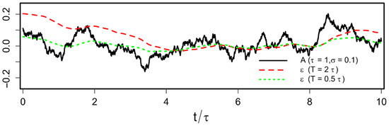
Figure 1. Evolution for the environmental fluctuations A (solid black line); and the population fluctuations for $T=2 \tau$ ($\Rightarrow \gamma =0.5/\tau$ ) (red dashed line), and $T=0.5 \tau$ ($\Rightarrow \gamma =2/\tau$ ) (green pointed line) for $\sigma =0.1$, $\lambda =1$ and $\tau =1$. Population fluctuations peak a short time after environmental fluctuations peak, indicating a delayed correlation between environmental and population fluctuations.

3. Temporal Autocorrelations and Cross-Correlations

Once we have seen the behavior of the evolution before, our target is to calculate temporal correlations for a single species in the presence of temporally autocorrelated noise. We want to calculate environmental (noise) autocorrelation, species autocorrelation, and environmental-species correlation, as well as a correlation time.

The correlation between two magnitudes $X$ and $Y$ in two instants separated by a delay $t\prime$ is given by the correlation function

$$c_{XY}\left(t^{\prime }\right)=<X\left(t\right)Y\left(t+t^{\prime }\right)>,$$

(3)

where $<>$ means expected value. This correlation indicates how good is $X\left(t\right)$ as a predictor of $Y\left(t+t^{\prime }\right)$. Therefore, to understand the predictability of the population fluctuations, we have computed the correlations functions of the environmental fluctuations $A$ and of the population fluctuations $\epsilon$. See Appendix A for the detail of the computations. The correlation functions are

$$c_{AA}\left(t^{\prime }\right)=\frac{{\sigma }^2}{2\tau }{e}^{-\left|t^{\prime }\right|/\tau }$$

(4)

$$c_{\epsilon \epsilon }\left(t^{\prime }\right)=\{\begin{array}{c}\frac{{\lambda }^2{\sigma }^2\tau }{2}\frac{{\alpha }^2}{1-{\alpha }^2}\left(e^{-\left|t^{\prime }\right|/\tau }-\alpha e^{-\left|t^{\prime }\right|/T}\right), T\ne \tau \\ \frac{{\lambda }^2{\sigma }^2\tau }{4}\left(1+\left|t^{\prime }\right|/\tau \right)e^{-\left|t^{\prime }\right|/\tau }, T=\tau \end{array}$$

(5)

$$c_{A\epsilon }\left(t^{\prime }\right)=\{\begin{array}{c}\frac{\lambda {\sigma }^2}{2}\frac{\alpha }{1+\alpha }{e}^{t^{\prime }/\tau }, t^{\prime }\le 0\\ \frac{\lambda {\sigma }^2}{2}\frac{\alpha }{1-{\alpha }^2}\left(\left(1+\alpha \right)e^{-t^{\prime }/\tau }-2\alpha e^{-t^{\prime }/T}\right), t\prime >0 \mathrm{and} T\ne \tau \\ \frac{\lambda {\sigma }^2}{4}\left(1+2t^{\prime }/\tau \right)e^{-t^{\prime }/\tau }, t\prime >0 \mathrm{and} T=\tau \end{array}$$

(6)

$$c_{\epsilon A}\left(t^{\prime }\right)=c_{A\epsilon }\left(-t^{\prime }\right)$$

(7)

where $\alpha =T/\tau =1/\left(\gamma \tau \right)$ is the dimensionless ratio between the characteristic damping time of the population fluctuations $T$ and the correlation time of the environmental fluctuations $\tau$. We have represented these correlation functions in Figure 2A.

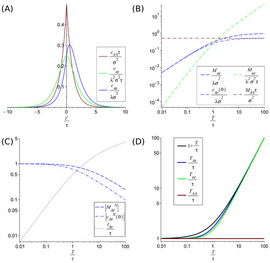
Figure 2. Correlation functions with their maximums and their values at t′ = 0 and correlation times. (A) represents the adimensionalized correlation functions $c_{\epsilon \epsilon }\left(t’\right)$ (green), $c_{AA}\left(t’\right)$ (red) and $c_{A\epsilon }\left(t’\right)$ (blue) adimensionalized for the case $\alpha =T/\tau =1$. (B) compares the adimensionalized maxima of the autocorrelations function $M_{AA}$ and $M_{\epsilon \epsilon }$ (which coincide with the value at $t^{\prime }=0$ of the respective autocorrelation) with the maxima of the adimensionalized crosscorrelation function $M_{A\epsilon }$ and its value at zero delay $c_{Aϵ}\left(0\right)$. Their normalized values, $M_{A\epsilon }^N=M_{A\epsilon }/\sqrt{c_{AA}\left(0\right)c_{\epsilon \epsilon }\left(0\right)}$ and $c_{A\epsilon }^N\left(0\right)=c_{A\epsilon }\left(0\right)/\sqrt{c_{AA}\left(0\right)c_{\epsilon \epsilon }\left(0\right)}$ are shown in (C), with the delay of the cross-correlation maximum $l_{A\epsilon }$. (D) compares the correlations times $T_{Aϵ}$, $T_{\epsilon \epsilon }$ and $T_{AA}$. These plots illustrate the hierarchies for temporal correlations and for the maxima of the correlations discussed in the main text. In particular, it shows that for low damping (large $\alpha =T/\tau$) the crosscorrelation time $T_{A\epsilon }$ increases, allowing longer-term predictions, despite the decrease in accuracy that can be seen from the decay of the normalized maximum of the crosscorrelation $M_{A\epsilon }^N$.

3.1. Maxima of the Correlation Functions

The autocorrelation function of the environmental fluctuations $c_{AA}\left(t^{\prime }\right)$ and the autocorrelation function of the species $c_{\epsilon \epsilon }\left(t^{\prime }\right)$, which are symmetric, have their maximum at the origin, $t^{\prime }=0$,

$$M_{AA}=c_{AA}\left(0\right)=\frac{{\sigma }^2}{2\tau }$$

(8)

$$M_{\epsilon \epsilon }=c_{\epsilon \epsilon }\left(0\right)=\frac{{\lambda }^2{\sigma }^2\tau }{2}\frac{{\alpha }^2}{1+\alpha }$$

(9)

The cross-correlation $c_{A\epsilon }\left(t^{\prime }\right)$, has a value at the origin of

$$c_{A\epsilon }\left(0\right)=\frac{\lambda {\sigma }^2}{2}\frac{\alpha }{1+\alpha }.$$

(10)

But the cross-correlation $c_{A\epsilon }\left(t^{\prime }\right)$ has a lagged maximum (a minimum for negative coupling $\lambda$), see Figure 2A, situated at a time displacement ($t^{\prime }=l_{A\epsilon })$

$$l_{A\epsilon }=\{\begin{array}{r}\tau \frac{\alpha }{1-\alpha }\ln \left(\frac{2}{1+\alpha }\right), T\ne \tau \\ \frac{\tau }{2}, T=\tau \end{array}$$

(11)

This lag means that the population is more affected by the fluctuation after a certain time instead of instantly. Because of the basic property of correlations $c_{XY}\left(t^{\prime }\right)=c_{YX}\left(-t^{\prime }\right)$, the correlation function $c_{A\epsilon }\left(t^{\prime }\right)$ has the maximum in $t^{\prime }=-l_{A\epsilon }$. This maximum is at $t’>0$ for any $\alpha =T/\tau >0$, and approaches the origin (smaller lag) as $T/\tau$ decreases. This dependence on $T/\tau$ causes the lag to tend to zero if the characteristic time of return to equilibrium of the population $T$ is very short.

The cross-correlation $c_{A\epsilon }\left(t^{\prime }\right)$ at this maximum located at $t^{\prime }=l_{Aϵ}$ has a value

$$M_{A\epsilon }=\{\begin{array}{r}\frac{\lambda {\mathsf{\sigma }}^2}{2} \alpha {\left(\frac{2}{1+\alpha }\right)}^{\frac{\alpha }{\alpha -1}}, T\ne \tau \\ \frac{\lambda {\sigma }^2}{2}{e}^{-1/2}, T=\tau \end{array}$$

(12)

It can be shown that the maximum correlation $M_{A\epsilon }$ at most doubles the correlation at the origin $c_{Aϵ}\left(0\right)$, i.e., $1\le \frac{M_{A\epsilon }}{c_{A\epsilon }\left(0\right)}\le 2$.

The maxima values can be adimensionalized and compared as in Figure 2B. This shows the following hierarchy

$$\begin{gathered} \frac{M_{\epsilon \epsilon }}{{\sigma }^2\tau }<\frac{M_{A\epsilon }}{\lambda {\sigma }^2}<\frac{M_{AA}\tau }{{\lambda }^2{\sigma }^2} \mathrm{for} T<\tau \\ \frac{M_{\epsilon \epsilon }}{{\sigma }^2\tau }\gtrsim \frac{M_{A\epsilon }}{\lambda {\sigma }^2}\gtrsim \frac{M_{AA}\tau }{{\lambda }^2{\sigma }^2} \mathrm{for} T\gtrsim \tau \end{gathered}$$

(13)

This hierarchy means that when the characteristic time scale of population fluctuations damping $T$ is greater than the environmental fluctuations correlation time $\tau ,$ the magnitude of the adimensionalized maxima increases as the fluctuation propagates (from the environment to the population). Conversely, when the population fluctuations dampen faster than the environmental fluctuations correlations time ($T<\tau$), the maxima decrease as the fluctuation propagates. Only in this later regime and when $T\ll \tau$ (i.e., on the constant environmental fluctuation limit) the normalized environment-population cross-correlation maximum reaches full correlation $M_{Aϵ}^N=1$ (but at zero delay, $l_{Aϵ}=0$). See Figure 2C. The normalized environment-population cross-correlation maximum and value at the origin are given by

$$M_{A\epsilon }^N=\frac{M_{A\epsilon }}{\sqrt{c_{AA}\left(0\right)c_{\epsilon \epsilon }\left(0\right)}}=\{\begin{array}{r}\mathrm{sign}\left(\lambda \right) \sqrt{2} {\left(\frac{2}{1+\alpha }\right)}^{\frac{1+\alpha }{2 \left(\alpha -1\right)}}, T\ne \tau \\ \mathrm{sign}\left(\lambda \right) \sqrt{2} e^{-1/2}, T=\tau \end{array}$$

(14)

$$c_{A\epsilon }^N\left(0\right)=\frac{c_{A\epsilon }\left(0\right)}{\sqrt{c_{AA}\left(0\right)c_{\epsilon \epsilon }\left(0\right)}}=\frac{\mathrm{sign}\left(\lambda \right)}{\sqrt{1+\alpha }}.$$

(15)

3.2. Temporal Correlations

The characteristic time of temporal correlations gives the time extension of the predictability. For simple exponential decays of the correlation, the correlation time is just given by the characteristic decay factor in the exponential. For more general cases, we define the correlation time as

$$T_{XY}=\frac{{{\displaystyle \int }}_0^{\infty }{t}^{\prime }\left|c_{XY}\left(t^{\prime }\right)\right|d{t}^{\prime }}{{{\displaystyle \int }}_0^{\infty }\left|c_{XY}\left(t^{\prime }\right)\right|d{t}^{\prime }}.$$

(16)

The absolute value allows incorporating the effects of negative correlations as predictors. For the autocorrelations and cross-correlations, we get

$$T_{AA}=T_{\epsilon A}=\tau$$

(17)

$$T_{\epsilon \epsilon }=\tau \left[1+\frac{{\alpha }^2}{1+\alpha }\right]=\tau +T\frac{1}{1+1/\alpha }$$

(18)

$$T_{A\epsilon }=\tau \left[1+\frac{2{\alpha }^2}{1+2\alpha }\right]=\tau +T\frac{1}{1+1/\left(2\alpha \right)}$$

(19)

In Figure 2D, these correlation times are plotted as functions of $\alpha =T/\tau$, the ratio between the damping time of the population fluctuations $T$ and the correlation time of the environmental fluctuations $\tau$. Figure 2D suggests a hierarchy of correlation times that can be proven from the previous expressions, i.e., Equations (17)–(19).

$$T_{AA}=T_{\epsilon A}=\tau <T_{\epsilon \epsilon }<T_{A\epsilon }<\tau +T$$

(20)

The difference between the last two is bounded by $0<\left(T_{A\epsilon }-T_{\epsilon \epsilon }\right)<\frac{\tau }{2}$.

This hierarchy of correlation times implies a longer correlation time, and therefore a larger scale of predictability, for population fluctuations than for environmental fluctuations.

4. Discussion

We aimed to understand the predictability of population fluctuations compared to environmental fluctuation predictability. To obtain an insight into the question, we computed the correlation functions of a population close to an equilibrium state in the presence of environmental colored noise. This computation allowed us to compute the correlation times and the maxima of the correlation functions, finding hierarchies for them, which gives general relations.

We found that the predictability of the population fluctuations is always higher than for the environmental fluctuations. Because of this, we have determined that the correlation time of the population fluctuations is always greater than the correlation time of the environmental fluctuations. The difference in correlation time increases with increased characteristic damping time of population fluctuations $T$. For example, for $T=10 \tau$ we have $T_{\epsilon \epsilon }=10.1 \tau$ and $T_{A\epsilon }=10.5 \tau$; we also have that the maximum of the population-environment cross-correlation is at $l_{A\epsilon }=1.9 \tau$ with a normalized correlation $M_{A\epsilon }^N=0.5$, showing a clear increase with respect to the correlation time for the environmental fluctuations $T_{AA}$. The underlying mechanism is analogous to the one described by Hasselmann for the integration of the fast weather components leading to the slow climate dynamics [30]. Our model stresses that the mechanism is general and time-scale independent. In practical cases times scales can range from days (for prey populations in agriculture) to years (for large species or ecosystems).

This study was inspired by our previous results on spatial population synchrony [31,32,33,34] and motivated by the findings that population fluctuations showed larger predictability than the underlying environmental variables. This was shown to happen for a wide range of systems: primary production in oceans [25], crop yield [26], malaria [27] and fisheries [28]. This higher predictability increases the prospects of predicting climatic variability effects on populations [26,27,28,35,36,37].

The determination of the effective equilibrium can be challenging in practical cases [24]. In general, the effective equilibrium is obtained from the time-average of the data in long-enough time series. However, sometimes the equilibrium can have seasonal oscillations or long-term trends. In this case, these variations in the equilibrium have to be taken into account, substracting them to obtain the correct fluctuations around equilibrium. Several model extensions are possible to obtain an insight into the scope of the results. The results have been obtained for a single-environmental variable acting on a single-species in the small fluctuation regime, which allows the linearization of the dynamical equations around the equilibrium. This model can be extended, including several interacting species and several environmental variables (which may also interact as wind stress and sea surface temperature). Another extension is including the division of species populations into distinct life stages, with some of them particularly affected by environmental fluctuations [38]. Our model considers small enough environmental fluctuations (which implies the population is close to equilibrium). This can be extended by studying larger environmental fluctuations in particularly relevant ecological models, which would clarify how the results in the present work are affected by the presence of nonlinearities.

The present study raises the question of how the propagation of fluctuations through the food webs impacts the predictability of the different species’ population fluctuations. This more profound understanding of the population predictability will help to design improved conservation policies, particularly useful for species especially sensitive to environmental variability (represented in our model with great couplings $\lambda$), such as ectotherms.

Appendix A.1. Wiener Process Temporal Autocorrelation

The temporal autocorrelation of the Wiener process (whose derivative gives the white noise) is known to be

$$c_{dWdW}\left(t^{\prime }\right)=\{\begin{array}{cc}dt,& \mathrm{for}{t}^{\prime }=0,\\ 0,& \mathrm{for}{\mathrm{t}}^{\prime }\ne 0.\end{array}$$

(A1)

Appendix A.2. Wiener—Colored-Noise Temporal Cross-Correlation

We now that $c_{dWA}\left(t^{\prime }\right)=<dW\left(t\right)A\left(t+t\prime \right)>$ is zero for $t^{\prime }\le 0$, as there is no fluctuation propagation to the past. Therefore, we just have to make the computation for positive time displacement.

We compute $c_{dWA}\left(t^{\prime }\right)=<dW\left(t\right)A\left(t+t\prime \right)>$ for $t^{\prime }=dt$, $t^{\prime }=2dt$, $t^{\prime }=3dt$, …

$$<dW\left(t\right)A\left(t+dt\right)>=<dW\left(t\right)\left(A\left(t\right)-\frac{A\left(t\right)}{\tau }dt+\frac{\sigma }{\tau }dW\left(t\right)\right)>=\frac{\sigma }{\tau } dt$$

$$<dW\left(t\right)A\left(t+2dt\right)>=<dW\left(t\right)\left(A\left(t+dt\right)-\frac{A\left(t+dt\right)}{\tau }dt+\frac{\sigma }{\tau }dW\left(t+dt\right)\right)>=\frac{\sigma }{\tau }\left(1-\frac{dt}{\tau }\right) dt$$

$$<dW\left(t\right)A\left(t+3dt\right)>=<dW\left(t\right)\left(A\left(t+2dt\right)-\frac{A\left(t+2dt\right)}{\tau }dt+\frac{\sigma }{\tau }dW\left(t+2dt\right)\right)>=\frac{\sigma }{\tau }{\left(1-\frac{dt}{\tau }\right)}^2 dt$$

These results allow us to get the general expression

$$c_{dWA}\left(ndt\right)=<dW\left(t\right)A\left(t+ndt\right)>=\frac{\sigma }{\tau }{\left(1-\frac{dt}{\tau }\right)}^{n-1} dt$$

In the large $n$ limit, we get the exponential expression

$$c_{dWA}\left(t^{\prime }\right)=\frac{\sigma }{\tau }{e}^{-t^{\prime }/\tau }dt \mathrm{if} t^{\prime }>0$$

Therefore, we have

$$c_{dWA}\left(t^{\prime }\right)=\{\begin{array}{c} 0 \mathrm{if} t^{\prime }\le 0\\ \frac{\sigma }{\tau }{e}^{-t^{\prime }/\tau } dt \mathrm{if} t^{\prime }>0\end{array}$$

(A2)

Appendix A.3. Wiener—Population Temporal Cross-Correlation

There is no propagation of the fluctuations to the past. Thus, $c_{dW\epsilon }\left(t^{\prime }\right)=<dW\left(t\right)\epsilon \left(t+t\prime \right)>$ is zero for $t^{\prime }\le 0$, and we only have to compute the correlation for positive time displacement.

The same procedure used for $c_{dWA}\left(t^{\prime }\right)$ allows obtaining $c_{dW\epsilon }\left(t^{\prime }\right)$

$$<dW\left(t\right)\epsilon \left(t+dt\right)>=<dW\left(t\right)·\left(\epsilon \left(t\right)-\gamma \epsilon \left(t\right)dt+\lambda A\left(t\right)dt\right)>=0$$

$$<dW\left(t\right)\epsilon \left(t+2dt\right)>=<dW\left(t\right)·\left(\epsilon \left(t+dt\right)-\gamma \epsilon \left(t+dt\right)dt+\lambda A\left(t+dt\right)dt\right)>=\frac{\lambda \sigma }{\tau }d{t}^2$$

$$<dW\left(t\right)\epsilon \left(t+3dt\right)>=<dW\left(t\right)·\left(\epsilon \left(t+2dt\right)-\gamma \epsilon \left(t+2dt\right)dt+\lambda A\left(t+2dt\right)dt\right)>=\frac{\lambda \sigma }{\tau }\left(1-\gamma dt\right)d{t}^2+\frac{\lambda \sigma }{\tau }\left(1-\frac{dt}{\tau }\right)d{t}^2$$

$$\begin{array}{r}<dW\left(t\right)\epsilon \left(t+4dt\right)>=<dW\left(t\right)·\left(\epsilon \left(t+3dt\right)-\gamma \epsilon \left(t+3dt\right)dt+\lambda A\left(t+3dt\right)dt\right)>\\ =\frac{\lambda \sigma }{\tau }{\left(1-\gamma dt\right)}^{2}d{t}^2+\frac{\lambda \sigma }{\tau }\left(1-\gamma dt\right)\left(1-\frac{dt}{\tau }\right)d{t}^2+\frac{\lambda \sigma }{\tau }{\left(1-\frac{dt}{\tau }\right)}^{2}d{t}^2\end{array}$$

$$<dW\left(t\right)\epsilon \left(t+ndt\right)>=\frac{d{t}^2}{\tau }\lambda \sigma {\displaystyle \sum }_{i=0}^{n-2}{\left(1-\gamma dt\right)}^{n-2-i}{\left(1-\frac{dt}{\tau }\right)}^i=\frac{\lambda \sigma }{\tau }d{t}^2{\left(1-\gamma dt\right)}^{n-2}{\displaystyle \sum }_{i=1}^{n-1}{\left(\frac{1-\frac{dt}{\tau }}{1-\gamma dt}\right)}^{i-1}$$

The later expression gives, when $\gamma \tau =1$

$$\frac{\lambda \sigma }{\tau }d{t}^2{\left(1-\gamma dt\right)}^{n-2}{\displaystyle \sum }_{i=1}^{n-1}1=\frac{\lambda \sigma }{\tau }d{t}^2{\left(1-\gamma dt\right)}^{n-2}·\left(n-1\right)\approx \frac{\lambda \sigma }{\tau }{t}^{\prime }{e}^{-\gamma t^{\prime }}dt=\frac{\lambda \sigma }{\tau }{t}^{\prime }{e}^{-t^{\prime }/\tau }dt,$$

while for $\gamma \tau \ne 1$

$$\begin{array}{l}\frac{\lambda \sigma }{\tau }d{t}^2{\left(1-\gamma dt\right)}^{n-2}{\displaystyle {\displaystyle \sum }_{i=1}^{n-1}}{\left(\frac{1-\frac{dt}{\tau }}{1-\gamma dt}\right)}^{i-1}=\frac{\lambda \sigma }{\tau }d{t}^2{\left(1-\gamma dt\right)}^{n-2}·\frac{1-{\left(\frac{1-\frac{dt}{\tau }}{1-\gamma dt}\right)}^{n-1}}{1-\frac{1-\frac{dt}{\tau }}{1-\gamma dt}}=\frac{\lambda \sigma dt}{1-\gamma \tau }\left({\left(1-\gamma dt\right)}^{n-1}-{\left(1-\frac{dt}{\tau }\right)}^{n-1}\right)\\ \hspace{1em}\hspace{1em}\hspace{1em}\hspace{1em}\hspace{1em}\hspace{1em}\hspace{1em}\approx \frac{\lambda \sigma }{1-\gamma \tau }\left(e^{-\gamma t^{\prime }}-e^{-t^{\prime }/\tau }\right)dt.\end{array}$$

(Note that in the limit $\gamma \tau \to 1,$ the results for $\gamma \tau =1$ are recovered, indicating the continuity of the solution on $\gamma \tau$.)

Therefore, we have the temporal correlation

$$c_{dW\epsilon }\left(t^{\prime }\right)=\{\begin{array}{c}0 \mathrm{if} t^{\prime }<0\\ \frac{\lambda \sigma }{1-\gamma \tau }\left(e^{-\gamma t^{\prime }}-e^{-t^{\prime }/\tau }\right)dt \mathrm{if} t^{\prime }>0 \mathrm{and} \gamma \tau \ne 1\\ \frac{\lambda \sigma }{\tau }{t}^{\prime }{e}^{-t^{\prime }/\tau }dt \mathrm{if} t^{\prime }>0 \mathrm{and} \gamma \tau =1\end{array}$$

(A3)

Appendix A.4. Colored-Noise Autocorrelations

The computation of this (and the following) temporal correlations relies on the time invariance of the dynamics, which leads to the stationarity of the asymptotic temporal correlations.

We begin calculating the temporal autocorrelation for the environmental autocorrelations, $c_{AA}\left(t^{\prime }\right)=<A\left(t\right)A\left(t+t^{\prime }\right)>$, whose stationary condition implies

$$\begin{gathered} <A\left(t\right)A\left(t+t^{\prime }\right)>=<\left(A\left(t\right)+dA\left(t\right)\right)·\left(A\left(t+t^{\prime }\right)+dA\left(t+t^{\prime }\right)\right)>= \\ <\left(A\left(t\right)-A\left(t\right)/\tau dt+\sigma /\tau dW\left(t\right)\right)·\left(A\left(t+t\prime \right)-A\left(t+t\prime \right)/\tau dt+\sigma /\tau dW\left(t+t\prime \right)\right)> \end{gathered}$$

Expanding up to the first order in $dt$ we get

$$\begin{gathered} <A\left(t\right)A\left(t+t^{\prime }\right)>=<A\left(t\right)A\left(t+t^{\prime }\right)>-\frac{2}{\tau }<A\left(t\right)A\left(t+t^{\prime }\right)>dt \\ +\frac{\sigma }{\tau }\left(1-\frac{dt}{\tau }\right)<A\left(t\right)dW\left(t+t^{\prime }\right)>+\frac{\sigma }{\tau }\left(1-\frac{dt}{\tau }\right)<dW\left(t\right)A\left(t+t^{\prime }\right)> \\ +\frac{{\sigma }^2}{{\tau }^2}<dW\left(t\right)dW\left(t+t^{\prime }\right)>, \end{gathered}$$

which gives the equation

$$\frac{2}{\tau }{c}_{AA}\left(t^{\prime }\right)dt=\frac{\sigma }{\tau }\left(1-\frac{dt}{\tau }\right)c_{AdW}\left(t^{\prime }\right)+\frac{\sigma }{\tau }\left(1-\frac{dt}{\tau }\right)c_{dWA}\left(t^{\prime }\right)+\frac{{\sigma }^2}{{\tau }^2}{c}_{dWdW}\left(t^{\prime }\right).$$

As we have shown that $c_{dWA}\sim dt$ and $c_{dWϵ}\sim dt$ [Equations (A2) and (A3)], which indicates that there are still terms of second order in the previous equation. Keeping only the first order terms in $dt$ and using $c_{AdW}\left(t^{\prime }\right)=c_{dWA}\left(-t^{\prime }\right)$, the equation becomes

$$c_{AA}\left(t^{\prime }\right)=\frac{\sigma }{2 dt} \left(c_{dWA}\left(t^{\prime }\right)+c_{dWA}\left(-t^{\prime }\right)\right)+\frac{{\sigma }^2}{2\tau }\frac{c_{dWdW}\left(t^{\prime }\right)}{dt}$$

This later equation gives $c_{AA}\left(t^{\prime }\right)$, in terms of the cross-correlations of the white noise with the colored noise and with the population fluctuations.

Substituting Equation (A2), we get environmental autocorrelation

$$c_{AA}\left(t^{\prime }\right)=\frac{{\sigma }^2}{2\tau }{e}^{-\left|t^{\prime }\right|/\tau }$$

(A4)

Appendix A.5. Colored-Noise—Population Cross-Correlation

We continue with the environment-species temporal cross-correlation $c_{A\epsilon }\left(t^{\prime }\right)=<A\left(t\right)\epsilon \left(t+t^{\prime }\right)>$, whose stationary condition gives

$$\begin{gathered} <A\left(t\right)\epsilon \left(t+t^{\prime }\right)>=<\left(A\left(t\right)+dA\left(t\right)\right)·\left(\epsilon \left(t+t^{\prime }\right)+d\epsilon \left(t+t^{\prime }\right)\right)>= \\ <\left(A\left(t\right)-A\left(t\right)/\tau dt+\sigma /\tau dW\left(t\right)\right)·\left(\epsilon \left(t+t\prime \right)-\gamma \epsilon \left(t+t\prime \right)dt+\lambda A\left(t+t\prime \right) dt\right)> \end{gathered}$$

Again, up to the first order in $dt$, we get

$$\begin{gathered} <A\left(t\right)\epsilon \left(t+t^{\prime }\right)>=<A\left(t\right)\epsilon \left(t+t^{\prime }\right)>-\left(\gamma +\frac{1}{\tau }\right)<A\left(t\right)\epsilon \left(t+t^{\prime }\right)>dt \\ +\frac{\sigma }{\tau }\left(1-\gamma dt\right)<dW\left(t\right)\epsilon \left(t+t^{\prime }\right)>+\lambda <A\left(t\right)A\left(t+t^{\prime }\right)>dt+\frac{\lambda \sigma }{\tau }<dW\left(t\right)A\left(t+t^{\prime }\right)>dt, \end{gathered}$$

resulting in the second relation,

$$-\left(\gamma +\frac{1}{\tau }\right)c_{A\epsilon }\left(t^{\prime }\right)dt+\frac{\sigma }{\tau }\left(1-\gamma dt\right)c_{dW\epsilon }\left(t^{\prime }\right)+\lambda c_{AA}\left(t^{\prime }\right)dt+\frac{\lambda \sigma }{\tau }{c}_{dWA}\left(t^{\prime }\right)dt=0.$$

Recalling again that $c_{dWA}\sim dt$ and $c_{dW\epsilon }\sim dt$, fewer terms are of the first order in $dt$, leading to

$$c_{A\epsilon }\left(t^{\prime }\right)=\frac{1}{\gamma +1/\tau } \left(\frac{\sigma }{\tau } \frac{c_{dW\epsilon }\left(t^{\prime }\right)}{dt}+\lambda c_{AA}\left(t^{\prime }\right)\right)$$

Substituting Equations (A3) and (A4), we can calculate the environmental-population fluctuations cross-correlation

$$c_{A\epsilon }\left(t^{\prime }\right)=\{\begin{array}{c}\frac{\lambda {\sigma }^2}{2\left(1+\gamma \tau \right)}{e}^{t^{\prime }/\tau }, t^{\prime }\le 0\\ \hfill \frac{\lambda {\sigma }^2}{2\left({\left(\gamma \tau \right)}^2-1\right)}\left(\left(1+\gamma \tau \right)e^{-t^{\prime }/\tau }-2e^{-\gamma t^{\prime }}\right), t^{\prime }>0 \mathrm{and} \gamma \tau \ne 1 \\ \hfill \frac{\lambda {\sigma }^2}{4\tau }\left(\tau +2t^{\prime }\right)e^{-t^{\prime }/\tau }, t^{\prime }>0 \mathrm{and} \gamma \tau =1\end{array}$$

(A5)

while $c_{\epsilon A}\left(t^{\prime }\right)=c_{A\epsilon }\left(-t^{\prime }\right)$.

Appendix A.6. Autocorrelations of the Population Fluctuations

We finally compute the temporal autocorrelation for the population fluctuations of the species $c_{\epsilon \epsilon }\left(t^{\prime }\right)=<\epsilon \left(t\right)\epsilon \left(t+t^{\prime }\right)>$, whose stationary condition implies

$$\begin{gathered} <\epsilon \left(t\right)\epsilon \left(t+t^{\prime }\right)>=<\left(\epsilon \left(t\right)+d\epsilon \left(t\right)\right)·\left(\epsilon \left(t+t^{\prime }\right)+d\epsilon \left(t+t^{\prime }\right)\right)>= \\ <\left(\epsilon \left(t\right)-\gamma \epsilon \left(t\right)dt+\lambda A\left(t\right) dt\right)·\left(\epsilon \left(t+t^{\prime }\right)-\gamma \epsilon \left(t+t^{\prime }\right)dt+\lambda A\left(t+t\prime \right) dt\right)>. \end{gathered}$$

Keeping terms up to first order in dt, we obtain the following expression:

$$\begin{gathered} <\epsilon \left(t\right)\epsilon \left(t+t^{\prime }\right)>=<\epsilon \left(t\right)\epsilon \left(t+t^{\prime }\right)>-2\gamma <\epsilon \left(t\right)\epsilon \left(t+t^{\prime }\right)>dt \\ +\lambda <\epsilon \left(t\right)A\left(t+t^{\prime }\right)>dt+\lambda <A\left(t\right)\epsilon \left(t+t^{\prime }\right)>dt \end{gathered}$$

In terms of correlations and using the relation $c_{XY}\left(t^{\prime }\right)=c_{YX}\left(-t^{\prime }\right)$, we have

$$c_{\epsilon \epsilon }\left(t^{\prime }\right)=\frac{\lambda }{2\gamma } \left(c_{A\epsilon }\left(t^{\prime }\right)+c_{A\epsilon }\left(-t^{\prime }\right)\right).$$

Substituting Equation (A5), we get for the population fluctuations autocorrelation

$$c_{\epsilon \epsilon }\left(t^{\prime }\right)=\{\begin{array}{r}\frac{{\lambda }^2{\sigma }^2\tau }{2\gamma \tau \left({\left(\gamma \tau \right)}^2-1\right)}\left(\gamma \tau e^{-\frac{\left|t^{\prime }\right|}{\tau }}-e^{-\gamma \left|t^{\prime }\right|}\right), \gamma \tau \ne 1\\ \frac{{\lambda }^2{\sigma }^2}{4}\left(\tau +\left|t^{\prime }\right|\right)e^{-\left|t^{\prime }\right|/\tau }, \gamma \tau =1\end{array}$$

(A6)

Appendix A.7. Maxima

The environmental noise autocorrelation $c_{AA}\left(t^{\prime }\right)$ and of the population fluctuations autocorrelation $c_{\epsilon \epsilon }\left(t^{\prime }\right)$ have their maximum at the origin $t^{\prime }=0$. The environment-population cross-correlation has a lagged maximum at a time $t^{\prime }=l_{A\epsilon }$ with

$$l_{A\epsilon }=\{\begin{array}{r}\frac{\ln \left(\frac{2\gamma \tau }{\gamma \tau +1}\right)}{\gamma \tau -1}\tau , \gamma \tau \ne 1\\ \frac{\tau }{2}, \gamma \tau =1\end{array}$$

(A7)

with a magnitude $M_{A\epsilon }=c_{A\epsilon }\left(l_{A\epsilon }\right)$ given by

$$M_{A\epsilon }=\{\begin{array}{r}\frac{\lambda {\sigma }^2{\left(\frac{2\gamma \tau }{1+\gamma \tau }\right)}^{\frac{1}{1-\gamma \tau }}}{2\gamma \tau }, \gamma \tau \ne 1\\ \frac{\lambda {\sigma }^2}{2}{e}^{-\frac{1}{2}}, \gamma \tau =1.\end{array}$$

(A8)

These expressions are also given in the main text in terms of $\alpha =\frac{T}{\tau }=\frac{1}{\gamma \tau }$, the ratio of the population relaxation time $T$ and the correlation time of environmental fluctuations $\tau$.

Appendix A.8. Correlation Times

The previous explicit expression for the time correlation function allows computing their respective correlation times

$$T_{AA}=\frac{{{\displaystyle \int }}_0^{\infty }{t}^{\prime }{c}_{AA}\left(t^{\prime }\right)d{t}^{\prime }}{{{\displaystyle \int }}_0^{\infty }{c}_{AA}\left(t^{\prime }\right)d{t}^{\prime }}=\frac{{{\displaystyle \int }}_0^{\infty }{t}^{\prime }\frac{{\sigma }^2}{2\tau }{e}^{-t^{\prime }/\tau }d{t}^{\prime }}{{{\displaystyle \int }}_0^{\infty }\frac{{\sigma }^2}{2\tau }{e}^{-t^{\prime }/\tau }d{t}^{\prime }}=\frac{{{\displaystyle \int }}_0^{\infty }{t}^{\prime }{e}^{-t^{\prime }/\tau }d{t}^{\prime }}{{{\displaystyle \int }}_0^{\infty }{e}^{-t^{\prime }/\tau }d{t}^{\prime }}=\tau ,$$

(A9)

$$T_{\epsilon A}=\tau ,$$

(A10)

$$T_{\epsilon \epsilon }=\tau \frac{{\left(\gamma \tau \right)}^2+\gamma \tau +1}{\gamma \tau \left(\gamma \tau +1\right)}=\tau \left[1+\frac{1}{\gamma \tau \left(\gamma \tau +1\right)}\right]=\tau \left[1+\frac{{\alpha }^2}{1+\alpha }\right]=\tau +T\frac{\alpha }{1+\alpha },$$

(A11)

$$T_{A\epsilon }=\tau \frac{{\left(\gamma \tau \right)}^2+2\gamma \tau +2}{\gamma \tau \left(\gamma \tau +2\right)}=\tau \left[1+\frac{2}{\gamma \tau \left(\gamma \tau +2\right)}\right]=\tau \left[1+\frac{2{\alpha }^2}{1+2\alpha }\right]=\tau +T\frac{2\alpha }{1+2\alpha },$$

(A12)

where $\alpha =\frac{T}{\tau }=\frac{1}{\gamma \tau }$ is the ratio of the population relaxation time $T$ and the correlation time of environmental fluctuations $\tau$.

References

- Gotelli, N.J. A Primer of Ecology, 4th ed.; Sinauer Associates: Sunderland, MA, USA, 2008. [Google Scholar]
- Lande, R.; Engen, S.; Saether, B.-E. Stochastic Population Dynamics in Ecology and Conservation. In Oxford Series in Ecology and Evolution; Oxford University Press: Oxford, UK, 2003. [Google Scholar] [CrossRef]
- Fujiwara, M.; Takada, T. Environmental Stochasticity. eLS 2017, 1–8. [Google Scholar] [CrossRef]
- Nowicki, P.; Bonelli, S.; Barbero, F.; Balletto, E. Relative Importance of Density-Dependent Regulation and Environmental Stochasticity for Butterfly Population Dynamics. Oecologia 2009, 161, 227–239. [Google Scholar] [CrossRef] [PubMed]
- Saltz, D.; Rubenstein, D.I.; White, G.C. The Impact of Increased Environmental Stochasticity Due to Climate Change on the Dynamics of Asiatic Wild Ass. Conserv. Biol. 2006, 20, 1402–1409. [Google Scholar] [CrossRef] [PubMed]
- Mangel, M.; Tier, C. Dynamics of Dynamics of Metapopulations with Demographic Stochasticity and Environmental Catastrophes. Theor. Popul. Biol. 1993, 44, 1–31. [Google Scholar] [CrossRef]
- Shaffer, M. Minimum Viable Populations: Coping with Uncertainty. In Viable Populations for Conservation; Cambridge University Press: Cambridge, UK, 1987; pp. 69–86. [Google Scholar] [CrossRef]
- Luis, A.D.; Douglass, R.J.; Mills, J.N.; Bjørnstad, O.N. Environmental Fluctuations Lead to Predictability in Sin Nombre Hantavirus Outbreaks. Ecology 2015, 96, 1691–1701. [Google Scholar] [CrossRef]
- Schreiber, S.J. Interactive Effects of Temporal Correlations, Spatial Heterogeneity and Dispersal on Population Persistence. Proc. R. Soc. B Biol. Sci. 2010, 277, 1907–1914. [Google Scholar] [CrossRef]
- Crespo-Miguel, R.; Jarillo, J.; Cao-García, F.J. Dispersal-induced resilience to stochastic environmental fluctuations in populations with Allee effect. Phys. Rev. E 2022, 105, 014413. [Google Scholar] [CrossRef]
- Petchey, O.L. Environmental Colour Affects Aspects of Single-Species Population Dynamics. Proc. R. Soc. B Boil. Sci. 2000, 267, 747–754. [Google Scholar] [CrossRef]
- Halley, J.M. Ecology, Evolution and 1f-Noise. Trends Ecol. Evol. 1996, 11, 33–37. [Google Scholar] [CrossRef]
- Ripa, J.; Lundberg, P. Noise Colour and the Risk of Population Extinctions. Proc. R. Soc. London 1996, 263, 1751–1753. [Google Scholar] [CrossRef]
- Heino, M.; Ripa, J.; Kaitala, V. Extinction Risk under Coloured Environmental Noise. Ecography 2000, 23, 177–184. [Google Scholar] [CrossRef]
- Greenman, J.V.; Benton, T.G. The Amplification of Environmental Noise in Population Models: Causes and Consequences. Am. Nat. 2003, 161, 225–239. [Google Scholar] [CrossRef] [PubMed]
- Kamenev, A.; Meerson, B.; Shklovskii, B. How Colored Environmental Noise Affects Population Extinction. Phys. Rev. Lett. 2008, 101, 268103. [Google Scholar] [CrossRef] [PubMed]
- Spanio, T.; Hidalgo, J.; A Muñoz, M. Impact of Environmental Colored Noise in Single-Species Population Dynamics. Phys. Rev. E 2017, 96, 042301. [Google Scholar] [CrossRef] [PubMed]
- Laakso, J.; Löytynoja, K.; Kaitala, V. Environmental Noise and Population Dynamics of the Ciliated Protozoa Tetrahymena Thermophila in Aquatic Microcosms. Oikos 2003, 102, 663–671. [Google Scholar] [CrossRef]
- Reuman, D.C.; Costantino, R.F.; Desharnais, R.A.; Cohen, J.E. Colour of Environmental Noise Affects the Nonlinear Dynamics of Cycling, Stage-Structured Populations. Ecol. Lett. 2008, 11, 820–830. [Google Scholar] [CrossRef] [PubMed]
- Zuo, W.; Moses, M.E.; West, G.B.; Hou, C.; Brown, J.H. A General Model for Effects of Temperature on Ectotherm Ontogenetic Growth and Development. Proc. R. Soc. B Boil. Sci. 2011, 279, 1840–1846. [Google Scholar] [CrossRef]
- Paaijmans, K.P.; Heinig, R.L.; Seliga, R.A.; Blanford, J.I.; Blanford, S.; Murdock, C.C.; Thomas, M.B. Temperature Variation Makes Ectotherms More Sensitive to Climate Change. Glob. Chang. Biol. 2013, 19, 2373–2380. [Google Scholar] [CrossRef]
- Atkinson, D. Temperature and Organism Size—A Biological Law for Ectotherms? Adv. Ecol. Res. 1994, 25, 1–58. [Google Scholar] [CrossRef]
- De Jong, G.; van der Have, T.M. Temperature Dependence of Development Rate, Growth Rate and Size: From Biophysics to Adaptation. In Phenotypic Plasticity of Insects: Mechanisms and Consequence; Science Publishers, Inc.: Plymouth, UK, 2009; pp. 461–526. [Google Scholar]
- Pimm, S.L.; Redfearn, A. The Variability of Population Densities. Nature 1988, 334, 613–614. [Google Scholar] [CrossRef]
- Séférian, R.; Bopp, L.; Gehlen, M.; Swingedouw, D.; Mignot, J.; Guilyardi, E.; Servonnat, J. Multiyear Predictability of Tropical Marine Productivity. Proc. Natl. Acad. Sci. USA 2014, 111, 11646–11651. [Google Scholar] [CrossRef] [PubMed]
- Capa-Morocho, M.; Rodríguez-Fonseca, B.; Ruiz-Ramos, M. Crop Yield as a Bioclimatic Index of El Niño Impact in Europe: Crop Forecast Implications. Agric. For. Meteorol. 2014, 198–199, 42–52. [Google Scholar] [CrossRef]
- Diouf, I.; Suárez-Moreno, R.; Rodríguez-Fonseca, B.; Caminade, C.; Wade, M.; Thiaw, W.M.; Deme, A.; Morse, A.P.; Ndione, J.-A.; Gaye, A.T.; et al. Oceanic Influence on Seasonal Malaria Incidence in West Africa. Weather Clim. Soc. 2022, 14, 287–302. [Google Scholar] [CrossRef]
- Gómara, I.; Rodríguez-Fonseca, B.; Mohino, E.; Losada, T.; Polo, I.; Coll, M. Skillful prediction of tropical Pacific fisheries provided by Atlantic Niños. Environ. Res. Lett. 2021, 16, 054066. [Google Scholar] [CrossRef]
- García-Ojalvo, J.; Sancho, J.M.; Ramírez-Piscina, L. Generation of spatiotemporal colored noise. Phys. Rev. A 1992, 46, 4670–4675. [Google Scholar] [CrossRef]
- Hasselmann, K. Stochastic Climate Models Part I. Theory. Theory. Tellus 1976, 28, 473–485. [Google Scholar] [CrossRef]
- Jarillo, J.; Saether, B.-E.; Engen, S.; Cao, F.J. Spatial Scales of Population Synchrony of Two Competing Species: Effects of Harvesting and Strength of Competition. Oikos 2018, 127, 1459–1470. [Google Scholar] [CrossRef]
- Jarillo, J.; Sæther, B.-E.; Engen, S.; Cao-García, F.J. Spatial Scales of Population Synchrony in Predator-Prey Systems. Am. Nat. 2020, 195, 216–230. [Google Scholar] [CrossRef]
- Lee, A.; Jarillo, J.; Peeters, B.; Hansen, B.; Cao-García, F.; Sæther, B.; Engen, S. Population Responses to Harvesting in Fluctuating Environments. Clim. Res. 2022, 86, 79–91. [Google Scholar] [CrossRef]
- Fernández-Grande, M.A.; Cao-García, F.J. Spatial Scales of Population Synchrony Generally Increases as Fluctuations Propagate in a Two Species Ecosystem. arXiv 2020, arXiv:2012.11043. Available online: https://arxiv.org/ftp/arxiv/papers/2012/2012.11043.pdf (accessed on 1 August 2022).
- Iizumi, T.; Luo, J.-J.; Challinor, A.; Sakurai, G.; Yokozawa, M.; Sakuma, H.; Brown, M.; Yamagata, T. Impacts of El Niño Southern Oscillation on the global yields of major crops. Nat. Commun. 2014, 5, 3712. [Google Scholar] [CrossRef] [PubMed]
- Watters, G.M.; Olson, R.J.; Francis, R.C.; Fiedler, P.C.; Polovina, J.J.; Reilly, S.B.; Aydin, K.Y.; Boggs, C.H.; E Essington, T.; Walters, C.J.; et al. Physical Forcing and the Dynamics of the Pelagic Ecosystem in the Eastern Tropical Pacific: Simulations with ENSO-Scale and Global-Warming Climate Drivers. Can. J. Fish. Aquat. Sci. 2003, 60, 1161–1175. [Google Scholar] [CrossRef][Green Version]
- Christensen, V.; Coll, M.; Buszowski, J.; Cheung, W.W.L.; Frölicher, T.; Steenbeek, J.; Stock, C.A.; Watson, R.; Walters, C.J. Oceanic Influence on Seasonal Malaria Incidence in West Africa. Glob. Ecol. Biogeogr. 2015, 24, 507–517. [Google Scholar] [CrossRef]
- Lowe, W.H.; Martin, T.E.; Skelly, D.K.; Woods, H.A. Metamorphosis in an Era of Increasing Climate Variability. Trends Ecol. Evol. 2021, 36, 360–375. [Google Scholar] [CrossRef] [PubMed]
Publisher’s Note: MDPI stays neutral with regard to jurisdictional claims in published maps and institutional affiliations. |
© 2022 by the authors. Licensee MDPI, Basel, Switzerland. This article is an open access article distributed under the terms and conditions of the Creative Commons Attribution (CC BY) license (https://creativecommons.org/licenses/by/4.0/).