Article

A Nonlinear Multigrid Method for the Parameter Identification Problem of Partial Differential Equations with Constraints

1
School of Mathematics and Statistics, Northeastern University at Qinhuangdao, Qinhuangdao 066000, China
2
School of Electrical and Electronic Engineering, Nanyang Technological University, Singapore 639798, Singapore
3
Eighth Geological Brigade of Hebei Bureau of Geology and Mineral Resources Exploration, Qinhuangdao 066000, China
*
Author to whom correspondence should be addressed.
Mathematics 2022, 10(16), 2938; https://doi.org/10.3390/math10162938
Submission received: 13 July 2022 / Revised: 7 August 2022 / Accepted: 12 August 2022 / Published: 15 August 2022
(This article belongs to the Special Issue Inverse Problems and Imaging: Theory and Applications)

Abstract

:
In this paper, we consider the parameter identification problem of partial differential equations with constraints. A nonlinear multigrid method is introduced to the process of parameter inversion. By keeping the objective functions on coarse grids consistent with those on fine grids, the proposed method reduces the dimensions of objective functions enormously and mitigates the risk of trapping in local minima effectively. Furthermore, constraints significantly improve the convergence ability of the method. We performed the numerical simulation based on the porosity identification of elastic wave equations in the fluid-saturated porous media, which suggests that the nonlinear multigrid method with constraints decreases the computational expenditure, suppresses the noise, and improves the inversion results.

1. Introduction

In science and engineering, the system of partial differential equations with unknown parameters, which cannot be measured directly, is often used to describe a physical model. An indispensable need for successfully modeling and optimizing the corresponding physical process is the accurate identification of unknown parameters. Normally, the values of these parameters are set at first on the base of laboratory experiments or literature data. Thereafter, comparing the results of the forward calculation of the system of partial differential equations (PDEs) with measurement data, the unknown parameters are determined by trial and error, such that the discrepancy is minimal.
Parameter identification inverse problem is widely applied in optical imaging [1,2], biomedical imaging [3,4], exploration seismology [5,6,7], groundwater flow modeling [8], industrial process monitoring [9,10], elasticity imaging [11,12], and acoustics imaging [13,14]. Owing to its nonlinearity and ill-posedness, such an inverse problem can hardly be solved explicitly. Recently, many authors focused on artificial intelligence algorithms, such as machine learning [15,16,17,18] and ensemble learning [19,20]. Moreover, there are traditional inversion algorithms such as gradient, Gauss–Newton, and full Newton methods [21,22,23,24], which are more often used on a fixed discretization grid. As long as there are more parameters needed to be estimated, the search space will increase and the computation efficiencies of these approaches will be lower. Motivated by the shortages of the above inversion methods, a nonlinear multigrid method was designed.
The multigrid method is an accurate and efficient method that has been successfully employed to solve forward and inverse problems [25,26]. When applied to inverse problems, the multigrid method can reduce the dimensions of objective functions enormously and mitigate the risk of trapping in local minima effectively by keeping the objective functions on coarse grids consistent with those on fine grids [27,28]. Inspired by the multigrid decomposition, Ye et al. [29] proposed a nonlinear multigrid optimization technique to reconstruct images in the field of optical diffusion tomography by computing the maximum a posteriori estimate. Marlevi et al. [30] utilized multigrid methods in tomographic image reconstruction from non-truncated projection data. Zhang et al. [31] studied an effective multigrid domain decomposition method in order to solve the minimization problem of the total variation. Zhang et al. [32] presented a multigrid correction scheme to obtain the solution to a new Steklov eigenvalue problem in inverse scattering. Edjlali et al. [33] applied the multigrid method to decrease the dimensions of the fluorescence tomographic imaging problem. A line search multigrid method was designed by Javaherian et al. [34] for photoacoustic tomography. Hu et al. [35] put forward a path covering adaptive algebraic multigrid method to solve linear systems of weighted graph Laplacians. The authors in [36,37,38] studied multigrid methods for the parameter identification problem of chemotaxis models inspired by Cancer-on-Chip experiments.
In comparison with using data only recorded on the surface of the studied object, the parameter inversion involving constraint data (such as the internal data of the object with a higher signal-to-noise ratio) might have lower noise levels and achieve better inversion quality. The parameter inversion with constraints has been applied in many areas including tectonophysics [39], geophysics [40,41], atmospheric research [42], remote sensing [43], and so on.
This article discusses the parameter identification problem of partial differential equations with constraints. Firstly, the problem was formulated as a constrained minimization problem, and then was converted to an unconstrained minimization problem by utilizing the penalty function method. Secondly, a V-cycle multigrid method with constraints (MGCS) was constructed for the parameter identification problem. Finally, the numerical simulation based on the porosity identification of elastic wave equations in the fluid-saturated porous media was carried out.
This article is organized in the following way. In Section 2, we briefly describe the constrained parameter inversion problem of partial differential equations. In Section 3, the details of MGCS are investigated. Section 4 is devoted to the numerical simulation performed for the porosity inversion of elastic wave equations in the fluid-saturated porous media. In Section 5, we present our conclusions and perspectives for future work.

2. Inversion Model

Consider a system of a partial differential equation
L ( p ( x ) , t ) u ( x , t ) = 0 , x Ω , 0 < t < T , E u ( x , 0 ) = φ ( x ) , x Ω , B u ( x , t ) = ϕ ( x , t ) , x Ω , 0 < t < T ,
where x = ( x 1 , x 2 , , x n ) is the space variable, t is the time variable, Ω R n is a bounded domain, Ω is the boundary of Ω , u ( x , t ) is a sufficiently smooth function defined on Ω × ( 0 , T ) . L, E, and B are, respectively, differential, initial condition, and boundary condition operators. u ( x , t ) can be determined with the known p ( x ) ; such a problem is denoted as a forward problem.
While the parameter p ( x ) is unknown, the process of identifying the unknown parameter p ( x ) from some observed data u o b s ( x b , t ) ( b = 1 , 2 , , B ) , which can be viewed as an optimization problem, is called the parameter identification inverse problem.
Firstly, solution u ( x , t ) of Equation (1) nonlinearly depends on p ( x ) , so a nonlinear operator equation can be defined as follows:
A ( p ( x ) ) = u ( x b , t ) ,
then, the parameter p ( x ) can be identified from the observed data u o b s ( x b , t ) by minimizing the discrepancy between the computed and observed data:
min A ( p ( x ) ) u o b s ( x b , t ) 2 .
In practical applications, the identified parameter and observed data in the problems are generally in discrete forms: for example, let
P = ( p 1 , p 2 , , p S ) , U o b s = ( u o b s ( x 1 , t ) , u o b s ( x 2 , t ) , , u o b s ( x B , t ) ) ,
denote the discrete forms of p ( x ) and u o b s ( x b , t ) , respectively.
To achieve better inversion quality, the constraint data (such as the internal data of the object with a higher signal-to-noise ratio) can be utilized. Denote the admissible set containing the constraint data p ^ i 1 , p ^ i 2 , , p ^ i J :
Φ = { P : p i j = p ^ i j , j = 1 , 2 , , J } ,
where 1 i 1 < i 2 < < i J S . Therefore, the parameter inversion with constraints is transformed into:
min P Φ A ( P ) U o b s 2 .
Assume
P ^ = ( p ^ i 1 , p ^ i 2 , , p ^ i J ) , D P = ( p i 1 , p i 2 , , p i J ) ,
where D is an extraction operator, such that D P P ^ = 0 by choice of P Φ . Hence, an output least squares problem without constraints is obtained:
min { A ( P ) U o b s 2 + μ 1 D P P ^ 2 } ,
where μ 1 denotes the constraint parameter, which can manage the constraint strength. In the specific inversion process, it is necessary to design a large enough μ 1 to ensure that the solution of Equation (5) is close to that of Equation (4).
Because of the ill-posedness of the inverse problem, the regularization technique has to be adopted to compute a stable approximation of the minimum, which leads to the associated least squares problem:
min H ( P ) = { A ( P ) U o b s 2 + μ 1 D P P ^ 2 + μ 2 P 2 } ,
where μ 2 denotes the regularization parameter, and the regularization term μ 2 P 2 is incorporated to enhance stability or provide priori information or both.

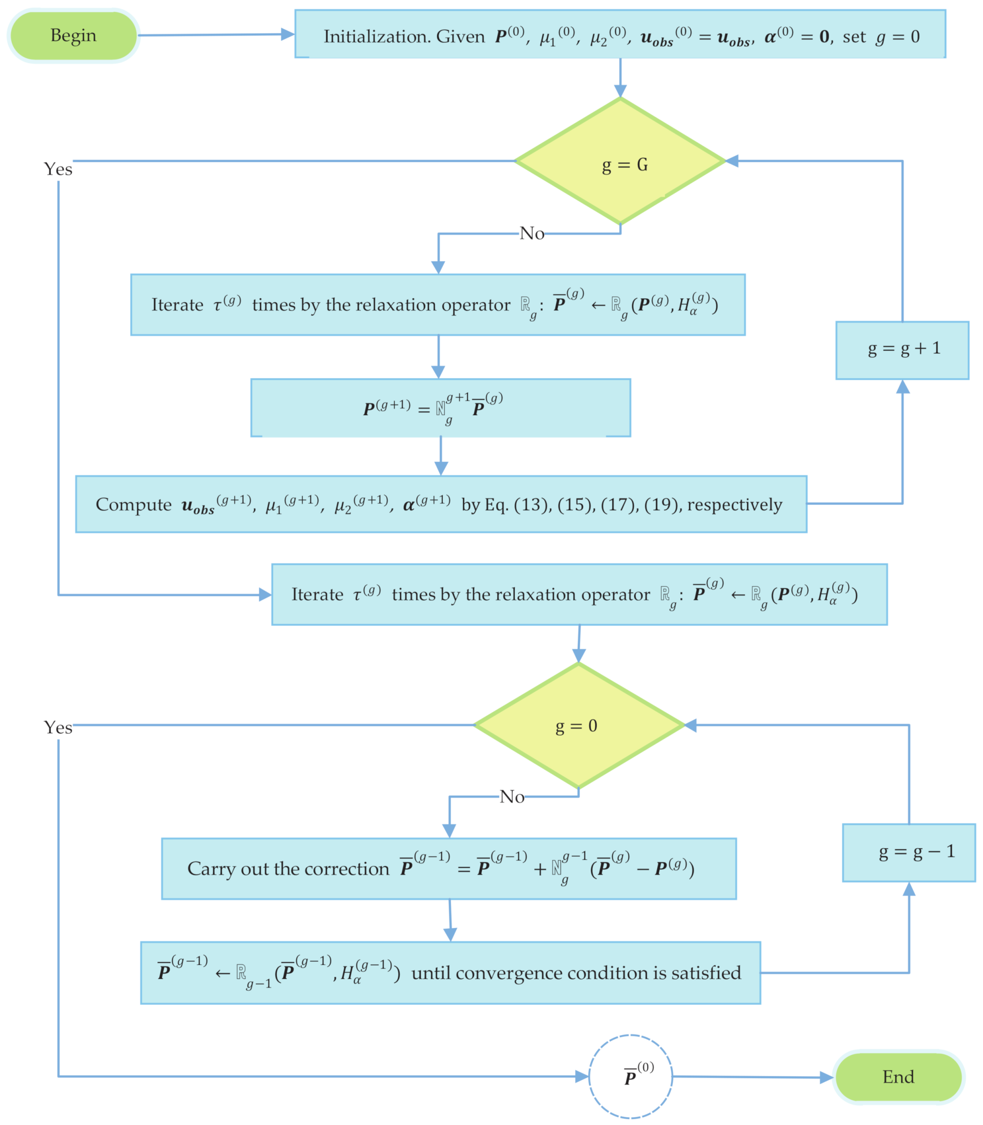
3. Multigrid Method with Constraints

As the primary component of the multigrid, a hierarchy of discretization grids is required:
{ Π g } , g = 0 , 1 , , G ,
where Π 0 is the finest grid, and Π g is attained with the discrete step size of Π 0 multiplied by 2 g . The objective functional is discretized on grid Π g :
H ( g ) ( P ( g ) ) = A ( g ) ( P ( g ) ) U o b s ( g ) 2 + μ 1 ( g ) D ( g ) P ( g ) P ^ ( g ) 2 + μ 2 ( g ) P ( g ) 2 ,
which has fewer local minima and lower dimensions on a coarser grid, to mitigate the risks of trapping in local minima and huge computations.
For the sake of propagating information between coarse and fine grids, we define the restriction and prolongation operators as
N g g + 1 : Π g Π g + 1 , g = 0 , 1 , , G 1 , N g + 1 g : Π g + 1 Π g , g = 0 , 1 , , G 1 .
For the sake of the parameter update on each fixed grid, we define the relaxation operators as
R g ( P ( g ) , H ( g ) ) ,
where P ( g ) is the initial value, H ( g ) is the objective function, and R g can be chosen as any iterative method, such as the regularized Gauss–Newton method [44], Levenberg–Marquardt method [45], and the Landweber method [46].
The coarser resolution approximation P ( g + 1 ) on grid Π g + 1 can be calculated by restricting the current approximation P ( g ) on grid Π g :
P ( g + 1 ) = N g g + 1 P ( g ) .
To improve P ( g ) , some τ ( g + 1 ) times iterations of the relaxation operator are performed with the initial value P ( g + 1 ) on the coarser grid Π g + 1 , and the result P ¯ ( g + 1 ) is denoted by
P ¯ ( g + 1 ) R g ( P ( g + 1 ) , H ( g + 1 ) ) ,
which is used to correct the finer grid approximation:
P ¯ ( g ) = P ( g ) + N g + 1 g ( P ¯ ( g + 1 ) N g g + 1 P ( g ) ) .
Although we expect that these operations lead to a more precise approximation, i.e., H ( g ) ( P ¯ ( g ) ) H ( g ) ( P ( g ) ) , it is hard to be tenable due to the possible inconsistent objective functionals. Therefore, some additional conditions are imposed to assure the monotonous convergence of MGCS.
Firstly, we add a correction term α ( g ) P ( g ) to the objective functionals to adjust their gradients:
H α ( g ) ( P ( g ) ) = H ( g ) ( P ( g ) ) α ( g ) P ( g ) = A ( g ) ( P ( g ) ) U o b s ( g ) 2 + μ 1 ( g ) D ( g ) P ( g ) P ^ ( g ) 2 + μ 2 ( g ) P ( g ) 2 α ( g ) P ( g ) ,
where α ( g ) is a row vector, and it is noteworthy that α ( 0 ) = 0 , so that H α ( 0 ) ( P ( 0 ) ) = H ( 0 ) ( P ( 0 ) ) .
Secondly, we restrict the initial discrepancy between the computed and observed data to be equal on the coarse and fine grids:
A ( g + 1 ) ( N g g + 1 P ( g ) ) U o b s ( g + 1 ) = A ( g ) ( P ( g ) ) U o b s ( g ) ,
then U o b s ( g + 1 ) is obtained from
U o b s ( g + 1 ) = U o b s ( g ) A ( g ) ( P ( g ) ) A ( g + 1 ) ( N g g + 1 P ( g ) ) ,
where the square bracket term compensates for the forward model mismatch on different grids.
Thirdly, we enforce the equal restriction on the constraint terms:
μ 1 ( g + 1 ) D ( g + 1 ) N g g + 1 P ( g ) P ^ ( g + 1 ) 2 = μ 1 ( g ) D ( g ) P ( g ) P ^ ( g ) 2 ,
which leads to the expression of μ 1 ( g + 1 )
μ 1 ( g + 1 ) = D ( g ) P ( g ) P ^ ( g ) 2 D ( g + 1 ) N g g + 1 P ( g ) P ^ ( g + 1 ) 2 μ 1 ( g ) ,
and again, on the regularization terms:
μ 2 ( g + 1 ) N g g + 1 P ( g ) 2 = μ 2 ( g ) P ( g ) 2 ,
which leads to the expression of μ 2 ( g + 1 )
μ 2 ( g + 1 ) = P ( g ) 2 N g g + 1 P ( g ) 2 μ 2 ( g ) .
Finally, the gradients of the fine and coarse grid objective functionals with the equal restriction is carried on so that the necessary condition of convergence of MGCS is satisfied:
H α ( g + 1 ) ( N g g + 1 P ( g ) ) = H α ( g ) ( P ( g ) ) N g + 1 g ,
with which one has
α ( g + 1 ) = H ( g + 1 ) ( N g g + 1 P ( g ) ) H α ( g ) ( P ( g ) ) N g + 1 g .
Note that, the right multiplication prolongation operator N g + 1 g works as the restriction operator.
A V-cycle MGCS can be developed with a recursive substitution—that another two-grid method is adopted instead of the iteration method on the coarser grid of the two-grid method. Figure 1 shows the flowchart.
To describe the V-cycle multigrid process, which is the significant recursion in an iteration procedure of our proposed method, a four-level grid with different spacing is used as an example in Figure 2. The iteration from the finest grid (0) to the coarsest grids (3) and then back to the finest grid (0) requires a recursive calling to Equations (8)–(10).

4. An Application

4.1. Mathematical Model

The performance of MGCS can be properly illustrated, with specific application to the porosity identification problem of elastic wave equations in the fluid-saturated porous media:
2 x κ u x x + z κ u x z + κ u z x + x λ u x x + λ u z z + x γ M w x x + γ M w z z = θ 2 u x t 2 + ρ f 2 w x t 2 f 1 , x κ u x z + κ u z x + 2 z κ u z z + z λ u x x + λ u z z + z γ M w x x + γ M w z z = θ 2 u z t 2 + ρ f 2 w z t 2 f 2 , x γ M u x x + γ M u z z + M w x x + M w z z = ρ f 2 u x t 2 + ϑ 2 w x t 2 f 1 , z γ M u x x + γ M u z z + M w x x + M w z z = ρ f 2 u z t 2 + ϑ 2 w z t 2 f 2 ,
with homogeneous initial conditions and homogeneous Neumann boundary conditions, where ( u x , u z ) , ( w x , w z ) are the solid-frame displacement and the fluid displacement relative to the solid-frame, respectively, and the considered domain Ω = [ 0 , L ] × [ 0 , H ] . Additionally,
γ = 1 B s B g , M = B g 2 D g B s , D g = B g 1 + p ( x , z ) B g B f 1 , θ = p ( x , z ) ρ f + 1 p ( x , z ) ρ s , ϑ = ρ f p ( x , z ) ,
where κ is the fluid viscosity, λ is the Lam e ´ coefficient, γ is the tortuosity, θ is the bulk density, ϑ is the mass density, ρ f is the pore fluid density, ρ s is the solid grain density, B s , B g , B f are, respectively, the bulk moduli of the skeletal frame, grain, and pore fluid, and p ( x , z ) is the porosity parameter to be identified. Porosity is a property that is associated with the subsurface media, so retrieving the porosity function can help explore the underground structure.
In practical applications, such as geophysical prospecting, the observed data are available at the earth’s surface (i.e., z = 0 ). Therefore, when Equation (20) is discretized by the finite difference method with spatial step lengths h x = L m x , h z = H m z , and time step length h t = T m t , we can obtain a vector-valued expression of the nonlinear operator Equation (2):
A ( P ) = U ,
where
P = ( p 0 , 0 , p 0 , 1 , , p 0 , m z , p 1 , 0 , p 1 , 1 , , p 1 , m z , , p m x , 0 , p m x , 1 , , p m x , m z ) , U = ( u x , 1 , 0 1 , u x , 2 , 0 1 , u x , m x 1 , 0 1 , u x , 1 , 0 2 , u x , 2 , 0 2 , u x , m x 1 , 0 2 , u x , 1 , 0 m t , u x , 2 , 0 m t , u x , m x 1 , 0 m t ) ,
and
p i , j = p ( i h x , j h z ) , u x , i , j k = u x ( i h x , j h z , k h t ) .
Let the observed data are arranged in the same way as U and form a vector expression U o b s , then this porosity parameter identification problem turns into
min A ( P ) U o b s 2 .
To achieve better inversion quality, the constraint data (porosity from the well logs of a well located at point i 0 in x) are introduced:
P ^ = ( p ^ i 0 , 0 , p ^ i 0 , 1 , , p ^ i 0 , m z ) .
Thus, the porosity parameter identification problem with the constraint can be written as
min { A ( P ) U o b s 2 + μ 1 D P P ^ 2 } ,
where
D = 0 0 0 1 0 0 0 0 0 0 0 0 0 1 0 0 0 0 0 0 0 0 0 1 0 0 0 ( m z + 1 ) × ( ( m x + 1 ) × ( m z + 1 ) )
such that
D P = ( p i 0 , 0 , p i 0 , 1 , , p i 0 , m z ) .

4.2. Simulation Test

There are some numerical simulation experiments presented to test MGCS and show its advantages, in contrast with the multigrid method without constraints (MG) and the fixed-grid method with constraints (FGCS). We choose
h x = 10 m , h z = 10 m , h t = 0.001 s , L = 400 m , H = 400 m , i 0 = 21 , μ 1 ( 0 ) = 10 3 , μ 2 ( 0 ) = 10 3 ,
to instantiate the above problem, with the source function and remaining involved parameters as in our previous paper [47].
Figure 3 presents the true porosity model used for our simulations. This model has two anomalous bodies in a homogeneous medium. The corresponding inversion results by MGCS and MG under four different Gauss noise levels of 30, 25, 20, and 15 dB are listed in Figure 4 and Figure 5, respectively. The color patterns on the charts mean the values of porosity as shown in the color box. In order to better compare the three methods (MGCS, MG, and FGCS) we give some detailed computational results (CPU execution times and relative errors of inversion results) in Table 1 and Table 2.
As seen from Table 1, under four different Gauss noise levels, the average CPU execution time of MGCS is 564.513 s, apparently lower than those of the two other methods. It is worth mentioning that the CPU execution times required for FGCS are almost double those of MGCS and MG, which means that the multigrid improves the calculation speed significantly. As 15 dB Gaussian noise is added, FGCS misses the global minimum, As 20 and 15 dB Gaussian noises are added, MG misses the global minimum. Therefore, it can be shown that MGCS is successful in mitigating the risk of trapping in local minima.
Table 2 demonstrates us that MGCS can achieve smaller relative errors of inversion results than MG and FGCS. With 20 dB of Gaussian noise added, the inversion results by MGCS and FGCS are satisfactory; however, MG cannot provide an acceptable inversion result. With 15 dB of Gaussian noise added, the inversion result by MGCS is still satisfactory; however, neither FGCS nor MG can provide an acceptable inversion result. This indicates that MGCS has a strong ability to suppress the noise. The reason for this is that MGCS combines the property of overcoming the disturbance of local minima of the multigrid method with the advantage of a high signal-to-noise ratio of the constraint data.

5. Conclusions

This study aimed to develop algorithms based on multigrid methods to solve the parameter identification inverse problem of partial differential equations with constraints. Firstly, in order to suppress the noise and achieve better inversion quality, the constraint data of lower noise levels were introduced to the parameter identification problems of PDEs. Secondly, we constructed a nonlinear multigrid method that improved the calculation speed and mitigated the risk of trapping in local minima. To evaluate the performance of this new method, we presented an application of that to the porosity identification of elastic wave equations in the fluid-saturated porous media. In summary, the advantages of the multigrid method with constraints are:
  • It is fast, accurate, and noise-resistant;
  • It is faster and less likely to fall into local minima compared to the multigrid method without constraints and fixed-grid method with constraints;
  • It has stronger anti-noise ability, higher precision, and better stability than the multigrid method without constraints and fixed-grid method with constraints.
The nonlinear multigrid method considered in this paper is mainly based on space discretization. The time domain multigrid method needs to be studied further. Constructing different multigrid methods will be an interesting part of future work.

Author Contributions

Conceptualization, T.L. and Y.Z.; methodology, T.L. and Y.Z.; software, T.L. and J.Y.; validation, T.L. and J.Y.; formal analysis, T.L. and J.Y.; investigation, T.L. and J.Y.; resources, Y.Y. and Y.Q.; data curation, T.L.; writing—original draft preparation, T.L., J.Y. and Y.Z.; writing—review and editing, T.L., J.Y. and Y.Z.; visualization, T.L.; supervision, Y.Z.; project administration, T.L., C.L. and Y.Q.; funding acquisition, T.L., C.L. and Y.Q. All authors have read and agreed to the published version of the manuscript.

Funding

This research was funded by the Natural Science Foundation of Hebei Province, China (A2020501007) and the Fundamental Research Funds for the Central Universities (N2123015).

Institutional Review Board Statement

Not applicable.

Informed Consent Statement

Not applicable.

Data Availability Statement

Not applicable.

Conflicts of Interest

The authors declare no conflict of interest.

References

  1. Zhu, L.; Soldevila, F.; Moretti, C.; d’Arco, A.; Boniface, A.; Shao, X.; de Aguiar, H.B.; Gigan, S. Large field-of-view non-invasive imaging through scattering layers using fluctuating random illumination. Nat. Commun. 2022, 13, 1447. [Google Scholar] [CrossRef] [PubMed]
  2. Boniface, A.; Dong, J.; Gigan, S. Non-invasive focusing and imaging in scattering media with a fluorescence-based transmission matrix. Nat. Commun. 2020, 11, 6154. [Google Scholar] [CrossRef] [PubMed]
  3. Göppel, S.; Frikel, J.; Haltmeier, M. Feature Reconstruction from Incomplete Tomographic Data without Detour. Mathematics 2022, 10, 1318. [Google Scholar] [CrossRef]
  4. Siddique, S.; Chow, J.C.L. Application of nanomaterials in biomedical imaging and cancer therapy. Nanomaterials 2020, 10, 1700. [Google Scholar] [CrossRef]
  5. Tromp, J. Seismic wavefield imaging of Earth’s interior across scales. Nat. Rev. Earth Environ. 2020, 1, 40–53. [Google Scholar] [CrossRef]
  6. Bringout, G.; Erb, W.; Frikel, J. A new 3D model for magnetic particle imaging using realistic magnetic field topologies for algebraic reconstruction. Inverse Probl. 2020, 36, 124002. [Google Scholar] [CrossRef]
  7. Yan, B.; Chen, B.; Harp, D.R.; Jia, W.; Pawar, R.J. A robust deep learning workflow to predict multiphase flow behavior during geological CO2 sequestration injection and Post-Injection periods. J. Hydrol. 2022, 607, 127542. [Google Scholar] [CrossRef]
  8. Kadeethum, T.; O’Malley, D.; Fuhg, J.N.; Choi, Y.; Lee, J.; Viswanathan, H.S.; Bouklas, N. A framework for data-driven solution and parameter estimation of PDEs using conditional generative adversarial networks. Nat. Comput. Sci. 2021, 1, 819–829. [Google Scholar] [CrossRef]
  9. Rymarczyk, T.; Niderla, K.; Kozłowski, E.; Król, K.; Wyrwisz, J.M.; Skrzypek-Ahmed, S.; Gołąbek, P. Logistic regression with wave preprocessing to solve inverse problem in industrial tomography for technological process control. Energies 2021, 14, 8116. [Google Scholar] [CrossRef]
  10. Rymarczyk, T.; Kozłowski, E.; Kłosowski, G. Electrical impedance tomography in 3D flood embankments testing–elastic net approach. Trans. Inst. Meas. Control 2020, 42, 680–690. [Google Scholar] [CrossRef]
  11. Jadamba, B.; Khan, A.A.; Richards, M.; Sama, M.; Tammer, C. Analyzing the role of the Inf-Sup condition for parameter identification in saddle point problems with application in elasticity imaging. Optimization 2020, 69, 2577–2610. [Google Scholar] [CrossRef]
  12. Jadamba, B.; Khan, A.A.; Richards, M.; Sama, M. A convex inversion framework for identifying parameters in saddle point problems with applications to inverse incompressible elasticity. Inverse Probl. 2020, 36, 074003. [Google Scholar] [CrossRef]
  13. Adeli, E.; Rosić, B.; Matthies, H.G.; Reinstädler, S.; Dinkler, D. Comparison of Bayesian methods on parameter identification for a viscoplastic model with damage. Metals 2020, 10, 876. [Google Scholar] [CrossRef]
  14. Frikel, J.; Haltmeier, M. Efficient regularization with wavelet sparsity constraints in photoacoustic tomography. Inverse Probl. 2018, 34, 024006. [Google Scholar] [CrossRef]
  15. Rymarczyk, T.; Król, K.; Kozłowski, E.; Wołowiec, T.; Cholewa-Wiktor, M.; Bednarczuk, P. Application of electrical tomography imaging using machine learning methods for the monitoring of flood embankments leaks. Energies 2021, 14, 8081. [Google Scholar] [CrossRef]
  16. Rymarczyk, T.; Kłosowski, G.; Hoła, A.; Sikora, J.; Wołowiec, T.; Tchórzewski, P.; Skowron, S. Comparison of machine learning methods in electrical tomography for detecting moisture in building walls. Energies 2021, 14, 2777. [Google Scholar] [CrossRef]
  17. Rymarczyk, T.; Kłosowski, G.; Hoła, A.; Hoła, J.; Sikora, J.; Tchórzewski, P.; Skowron, Ł. Historical buildings dampness analysis using electrical tomography and machine learning algorithms. Energies 2021, 14, 1307. [Google Scholar] [CrossRef]
  18. Rymarczyk, T.; Kozłowski, E.; Kłosowski, G.; Niderla, K. Logistic regression for machine learning in process tomography. Sensors 2019, 19, 3400. [Google Scholar] [CrossRef]
  19. Rymarczyk, T.; Kłosowski, G. Identification of moisture inside walls in buildings using machine learning and ensemble methods. Int. J. Appl. Electrom. 2022, 69, 375–388. [Google Scholar] [CrossRef]
  20. Kłosowski, G.; Rymarczyk, T. Ensemble learning for monitoring process in electrical impedance tomography. Int. J. Appl. Electrom. 2022, 69, 169–178. [Google Scholar] [CrossRef]
  21. Markl, M.; Alley, M.T.; Pelc, N.J. Balanced phase-contrast steady-state free precession (PC-SSFP): A novel technique for velocity encoding by gradient inversion. Magn. Reson. Imaging 2003, 49, 945–952. [Google Scholar] [CrossRef] [PubMed]
  22. Liu, T. A wavelet multiscale-homotopy method for the parameter identification problem of partial differential equations. Comput. Math. Appl. 2016, 71, 1519–1523. [Google Scholar] [CrossRef]
  23. Schweiger, M.; Arridge, S.R.; Nissilä, I. Gauss-Newton method for image reconstruction in diffuse optical tomography. Phys. Med. Biol. 2005, 50, 2365. [Google Scholar] [CrossRef] [PubMed]
  24. Pan, W.; Innanen, K.A.; Margrave, G.F.; Fehler, M.C.; Fang, X.; Li, J. Estimation of elastic constants for HTI media using Gauss-Newton and full-Newton multiparameter full-waveform inversion. Geophysics 2016, 81, R275–R291. [Google Scholar] [CrossRef]
  25. Lee, C.; Jeong, D.; Yang, J.; Kim, J. Nonlinear multigrid implementation for the two-dimensional Cahn-Hilliard equation. Mathematics 2020, 8, 97. [Google Scholar] [CrossRef]
  26. Liu, T. A multigrid-homotopy method for nonlinear inverse problems. Comput. Math. Appl. 2020, 79, 1706–1717. [Google Scholar] [CrossRef]
  27. Oh, S.; Milstein, A.B.; Bouman, C.A.; Webb, K.J. A general framework for nonlinear multigrid inversion. IEEE Trans. Image Process. 2005, 14, 125–140. [Google Scholar]
  28. Liu, T. Parameter estimation with the multigrid-homotopy method for a nonlinear diffusion equation. J. Comput. Appl. Math. 2022, 413, 114393. [Google Scholar] [CrossRef]
  29. Ye, J.C.; Bouman, C.A.; Webb, K.J.; Millane, R.P. Nonlinear multigrid algorithms for Bayesian optical diffusion tomography. IEEE Trans. Image Process. 2001, 10, 909–922. [Google Scholar]
  30. Marlevi, D.; Kohr, H.; Buurlage, J.; Gao, B.; Batenburg, K.J.; Colarieti-Tosti, M. Multigrid reconstruction in tomographic imaging. IEEE Trans. Radiat. Plasma 2020, 4, 300–310. [Google Scholar] [CrossRef]
  31. Zhang, Z.; Li, X.; Duan, Y.; Yin, K.; Tai, X.C. An efficient multi-grid method for TV minimization problems. Inverse Probl. Imag. 2021, 15, 1199–1221. [Google Scholar] [CrossRef]
  32. Zhang, Y.; Bi, H.; Yang, Y. A multigrid correction scheme for a new Steklov eigenvalue problem in inverse scattering. Int. J. Comput. Math. 2020, 97, 1412–1430. [Google Scholar] [CrossRef]
  33. Edjlali, E.; Bérubé-Lauzière, Y. Lq-Lp optimization for multigrid fluorescence tomography of small animals using simplified spherical harmonics. J. Quant. Spectrosc. Ra. 2018, 205, 163–173. [Google Scholar] [CrossRef]
  34. Javaherian, A.; Holman, S. A multi-grid iterative method for photoacoustic tomography. IEEE Trans. Med. Imaging 2017, 36, 696–706. [Google Scholar] [CrossRef] [PubMed]
  35. Hu, X.; Lin, J.; Zikatanov, L.T. An adaptive multigrid method based on path cover. SIAM J. Sci. Comput. 2019, 41, 220–241. [Google Scholar] [CrossRef]
  36. Braun, E.C.; Bretti, G.; Natalini, R. Parameter estimation techniques for a chemotaxis model inspired by Cancer-on-Chip (COC) experiments. Int. J. Nonlin. Mech. 2022, 140, 103895. [Google Scholar] [CrossRef]
  37. Braun, E.C.; Bretti, G.; Natalini, R. Mass-preserving approximation of a chemotaxis multi-domain transmission model for microfluidic chips. Mathematics 2021, 9, 688. [Google Scholar] [CrossRef]
  38. Bretti, G.; De Ninno, A.; Natalini, R.; Peri, D.; Roselli, N. Estimation algorithm for a hybrid PDEODE model inspired by immunocompetent Cancer-on-Chip experiment. Axioms 2021, 10, 243. [Google Scholar] [CrossRef]
  39. Christiansen, R.; Morosini, A.; Enriquez, E.; Muñoz, B.; Klinger, F.L.; Martinez, M.P.; Suárez, A.O.; Kostadinoff, J. 3D litho-constrained inversion model of southern Sierra Grande de San Luis: New insights into the Famatinian tectonic setting. Tectonophysics 2019, 756, 1–24. [Google Scholar] [CrossRef]
  40. Aragao, O.; Sava, P. Elastic full-waveform inversion with probabilistic petrophysical model constraints. Geophysics 2020, 85, 101–111. [Google Scholar] [CrossRef]
  41. Mahmoodi, O.; Smith, R.S.; Spicer, B. Using constrained inversion of gravity and magnetic field to produce a 3D litho-prediction model. Geophys. Prospect. 2017, 65, 1662–1679. [Google Scholar] [CrossRef]
  42. Gao, L.; Sadeghi, M.; Ebtehaj, A. Microwave retrievals of soil moisture and vegetation optical depth with improved resolution using a combined constrained inversion algorithm: Application for SMAP satellite. Remote Sens. Environ. 2020, 239, 111662. [Google Scholar] [CrossRef]
  43. Ebtehaj, A.; Bras, R.L. A physically constrained inversion for high-resolution passive microwave retrieval of soil moisture and vegetation water content in L-band. Remote Sens. Environ. 2019, 233, 111346. [Google Scholar] [CrossRef]
  44. Abubakar, A.; Habashy, T.M.; Pan, G.D.; Li, M. Application of the multiplicative regularized Gauss-Newton algorithm for three-dimensional microwave imaging. IEEE Trans. Antenn. Propag. 2012, 60, 2431–2441. [Google Scholar] [CrossRef]
  45. Yan, Z.; Zhong, S.; Lin, L.; Cui, Z. Adaptive Levenberg-Marquardt algorithm: A new optimization strategy for Levenberg-Marquardt neural networks. Mathematics 2021, 9, 2176. [Google Scholar] [CrossRef]
  46. Zhang, R.; Li, F.; Luo, X. Multiscale compression algorithm for solving nonlinear ill-posed integral equations via Landweber iteration. Mathematics 2020, 8, 221. [Google Scholar] [CrossRef]
  47. Liu, T. Porosity reconstruction based on Biot elastic model of porous media by homotopy perturbation method. Chaos Solitons Fractals 2022, 158, 112007. [Google Scholar] [CrossRef]
Figure 1. The flowchart of MGCS.
Mathematics 10 02938 g001
Figure 2. The V-cycle multigrid iteration process.
Mathematics 10 02938 g002
Figure 3. The true model.
Mathematics 10 02938 g003
Figure 4. The inversion results by MGCS with different noise levels; (ad) are the identified porosity images with 30, 25, 20, and 15 dB Gaussian noises, respectively.
Mathematics 10 02938 g004
Figure 5. The inversion results by MG with different noise levels; (a,b) are the identified porosity images with 30 and 25 dB Gaussian noises, respectively.
Mathematics 10 02938 g005
Table 1. The CPU execution times (seconds) by three different methods.
Noise LevelMGCSMGFGCS
30 dB531.191633.2751038.302
25 dB586.140623.0601002.997
20 dB571.452×1071.707
15 dB569.270××
Table 2. The relative errors of inversion results from three different methods.
Noise LevelMGCSMGFGCS
30 dB0.02130.06350.0373
25 dB0.02970.08130.0415
20 dB0.0331×0.0493
15 dB0.0593××
Publisher’s Note: MDPI stays neutral with regard to jurisdictional claims in published maps and institutional affiliations.

