An Interval-Simplex Approach to Determine Technological Parameters from Experimental Data

Abstract

Statistical equations are widely used to describe the laws of various chemical technological processes. The values of constants and parameters included in these equations are determined by various methods. Methods that can determine the values of equation parameters using a limited amount of experimental data are of particular practical interest. In this manuscript, we propose a method to obtain simplex-interval equations. The proposed approach can be effectively used to control the values of technological process parameters. In this paper, we consider examples of chemical kinetics equation transformations and heterogeneous processes of solid particle dissolution. In addition, we describes mathematical model transformations, including equations for functions of the residence time distribution (RTD) of apparatus particles, the distribution of particles by size, etc. Finally, we apply the proposed approach to an example involving modeling of the calcination of coke in a tubular rotary kiln.

1. Introduction

Fundamental analytical dependencies are necessary to determine performance indicators of technological processes. Adequate mathematical models can be created by considering the peculiarities of chemical reactions and mass transfer course. In engineering practice, differential equations of various orders are used to create mathematical models. The numerical solution of such equations is difficult in most cases. Therefore, when a direct solution is impossible, equations and their boundary conditions are analyzed in order to formulate approximate solutions in the form of a similarity criteria general function. Similarity criteria are usually derived either by analyzing differential equations, describing the process under study and their boundary conditions, or using the dimensional analysis method.

The method of dimensional analysis is supplemented by expert assessment to increase the reliability of obtained characteristics of complex processes in engineering design practice [1,2,3]. The disadvantages of these methods ultimately lead to attainment of approximate equations describing the process, limiting their applicability in engineering calculation practice [4].

In connection with the approximate nature of the criterion equations obtained by this method, the development of a method for transforming equations into a criterial form is of practical and theoretical interest. Therefore, in this article, we propose a new approach using the simplex method.

The efficiency of chemical and metallurgical apparatus depends not only on the technological mode but also on design features, which determine the final result [5,6]. To determine the optimal design and dimensions of an apparatus, it is necessary to take into consideration the chemical reactions rates, heat and mass transfer, and the hydrodynamic mode or flow behavior of the apparatus.

Optimization methods, such as artificial neural networks [7,8,9], the simplex method [10,11,12,13], and genetic algorithms [14,15,16], as well as various combinations thereof [17,18], provide effective means of determining the optimal values of process parameters, leading to optimal conditions. Such methods differ in terms of the height of the determined optimum, the number of experiments, and the required time.

Batch, semi-periodic, and continuous reactors are commonly used in modern industrial chains. Continuous reactors are most effective due to superior unit productivity and continuous automated operation and control ability. Batch units are usually used only in industries with small reaction phase flows. The economic efficiency of the latter mostly depends on appropriate configuration of technological reactor and process parameter values [3,13,15,19,20].

Residence time distribution modeling is used for various chemical engineering processes, for example, to describe the full cycle of a continuous production line or the complex behavior of a single unit in a technological chain. Mathematical models of multiple connected ideal or non-ideal reactors with a known analytical RTD are used in major cases. The most common types are continuous stirred tank reactors (CSTRs) and plug flow reactors (PFRs). However, these reactor types are too idealized for correct modeling of the behavior of real processes. Therefore, a combination of various models takes into account the characteristics of fluid flow, including effects such as dead zones, non-ideal back mixing, and bypassing effects. Furthermore, the determination of combined model parameters is complicated. Non-linear programming methods are used for such task. The proposed approach of RTD modeling is used, for example, in the development of chemical reactions, metallurgy, pharmaceuticals, water purification processes, etc. [21,22,23,24].

The main factors influencing any type of apparatus operation include:

(1)

Thermodynamic factors: constants of chemical and phase equilibrium. This group of factors determines the reaction direction and technological parameters and affects the rate and selectivity of the entire process [25];

(2)

Kinetic factors: rate constants and activation energies of the main and side reactions, as well as the reaction’s true and apparent orders [4,25];

(3)

Mass transfer factors: mass transfer coefficients of initial and intermediate substances and final reaction products [6,26];

(4)

Heat exchange factors: heat transfer coefficients within phases and between the medium and heat exchange devices, as well as the external heat exchange surface size [15];

(5)

Hydrodynamic factors: interface characteristics and mixing in continuous and dispersed phases [3,25].

The last factor in the above list plays the main role, as the hydrodynamic environment decisively affects the heat rate and mass transfer processes, as well as the chemical process rate [4,26].

The operation of technological equipment is characterized by close connections between productivity, quality, and production cost. The latter depends on the optimal time of the raw material’s actual stay in the apparatus. With an unjustified delay of raw materials in the apparatus, the equipment’s overall performance decreases, production cost increases, and in some cases, the product quality can also decrease [26,27]. Although an unjustified reduction in RTD increases the overall performance of the equipment, it reduces the efficiency of the raw processing material, leading to a deterioration in product quality.

To determine the mathematical model parameters for a continuous reactor, it is first necessary to consider the RTD of the material in the apparatus, which will ultimately improve the economic efficiency of the process under consideration. Information about RTD in the apparatus enables evaluation of the efficiency of the apparatus itself, which determines the proportion of the apparatus volume occupied by particles within a given time interval [28,29,30].

Various methods have been applied to analyze complex systems of differential equations, describing the phenomenon or process under study. The methods used with respect to similarity theory are of the most practical interest. As an example, consider the possibility of using simplex-interval methods for equations of chemical kinetics; heterogeneous processes of dissolution of solid particles; and transformations of mathematical models, including equations for the RTD functions of particles in an apparatus, equations for particles size distribution, etc. [31,32,33,34,35]. The interval method affords simplex-interval equations. It can be effectively used to control the values of technological and chemical process parameters [36,37,38].

In this paper, we consider the use of the simplex-interval method to convert statistical equations of varying complexity into a convenient form for practical engineering calculations. To that end, it is necessary to determine the values of constants and parameters included in these equations. In the future, such a method could enable the development of an automatic control system using model-predictive controllers in a dynamic mode [39,40].

2. Materials and Methods

According to the simplex-interval method, statistical equations describing the kinetics of chemical and metallurgical processes can be converted to a dimensionless form through similarity simplices corresponding to several values of $y_i$ and $x_i$ selected on the experimental curve $y_i=\phi \left(x_i\right)$ describing the investigated process. For example, any two values of the functions $y_i$ and $y_{i+1}$ corresponding to two values of the arguments $x_i$ and $x_{i+1}$ determined from an experimental curve can be expressed as [41]:

(1)

For the value of the argument $x_i,x_i=\phi \left(y_i\right)$; and

(2)

For the value of the argument $x_{i+1},x_{i+1}=\phi \left(y_{i+1}\right)$.

For the interval considered above, $\Delta x=x_{i+1}-x_i$, the form of the functional dependence $\Delta x, S_x, X_a, X_g$ and others can be determined from $y_i$ and $y_{i+1}$, where $\Delta x$ is the value of the interval used to calculate the parameters of the equation; $X_a$ and $X_g$ are the arithmetic mean and geometric mean of $x_i$ and $x_{i+1}$, respectively; and $S_x$ is the similarity simplex.

The equation system solution affords a simplex-interval dependence that describes the investigated technological process laws.

The simplex-interval equation can also be obtained using the following interval characteristics: $\Delta y$, $S_y$,$y_a=\left(y_{i+1}·y_i\right)/2$ and $y_g=\sqrt{y_{i+1}·y_i}$, as determined for the interval of variation of the value $\Delta y=y_i-y_{i+1}$. To determine the characteristics $∆y/∆x=f\left(x_i;x_{i+1}\right)$ and $∆y·∆x=f\left(x_i;x_{i+1}\right)$, it is necessary to identify expressions that afford a generalized description.

The proposed simplex-interval method makes it possible to determine the values of the parameters of the equations using a limited number of experimental points (for example, with two or three values of $x_i$ corresponding to two or three values of $y_i$), provided that

For the interval $\Delta x$, the form of the functional dependence $\Delta x=\phi \left(y\right)$ and similarity simplex $S_y=\phi \left(y\right)$ can be expressed as:

$$\Delta x=x_{i+1}-x_i={\varphi }_1\left(y;y_{i+1}\right),$$

(1)

$$S_y=x_{i+1}/x_i={\varphi }_2\left(y_i;y_{i+1}\right),$$

(2)

The joint solution of Equations (1) and (2) affords a simplex-criteria dependence describing the laws of the process under study. The possibility of applying the simplex-interval method to transform equations describing metallurgical and chemical process laws is illustrated by the examples in presented in the Results section.

3. Results

3.1. Simplex-Interval Method Examples

For a reaction of zero order, the laws of which are described by the kinetic equation (n = 0):

$$\frac{c}{c_0}=1-k_0\frac{\tau }{c_0},$$

(3)

where $c_0$ and c are the concentration of the target component at time τ = 0 and τ, respectively; and $k_0$ is the specific reaction rate of the zero order.

We define the interval characteristics as $\Delta \tau$ and $\Delta c$. The simplex-criteria equation for the case under consideration will have the form

$$-\frac{\Delta c}{\Delta \tau }=k_0,$$

(4)

For a first order reaction (n = 1)

$$\frac{c}{c_0}=exp(-k_1\tau ),$$

(5)

where k₁—the first-order reaction rate.

The values of the interval characteristics $\Delta \tau , \Delta c,S_{\tau }, \mathrm{and} S_c$ for any two points lying on the kinetic curve can be determined by the following formulae:

$$\Delta \tau =\left(1/k_1\right)ln{S}_c^{-1},$$

(6)

where is the similarity simplex for concentration matter.

And

$$\Delta c=c_0\left(S_c^{\frac{S_{\tau }}{S_{\tau }-1}}-S_c^{\frac{1}{S_{\tau }-1}}\right),$$

(7)

where $S_{\tau }$ is similarity simplex for time.

Combining dependences (6) and (7) result in:

$$-\frac{\Delta c}{\Delta \tau }=k_1{c}_0\left(S_c^{\frac{S_{\tau }}{S_{\tau }-1}}-S_c^{1/\left(S_{\tau }-1\right)}\right){/lnS}_c,$$

(8)

For a second-order reaction (n = 2)

$$\frac{c}{c_0}=\frac{1}{1+c_0{k}_1\tau },$$

(9)

where k₂ is the second-order reaction rate.

Similarly, the values of the interval characteristics are related by the following dependencies:

$$\Delta \tau =\left(\frac{1}{k_2{c}_0}\right)\frac{\left(1-S_c\right)(S_{\tau }-1)}{S_c{S}_{\tau }-1},$$

(10)

and

$$\Delta c=c_0\left(\frac{\left(S_c{S}_{\tau }-1\right)(S_{\tau }-1)}{S_c(S_{\tau }-1)}\right),$$

(11)

The ratio $\Delta c/\Delta \tau$ in this case is determined by:

$$-\frac{\Delta c}{\Delta \tau }=k_2{C}_0^2\frac{{(S_c{S}_{\tau }-1)}^2}{S_c{(S_{\tau }-1)}^2},$$

(12)

In the general case, for reactions of order (n > 1)

$$\frac{c}{c_0}={\left(\frac{1}{1+\left(n-1\right)k_n{c}_0^{n-1}\tau }\right)}^{1/\left(n-1\right)},$$

(13)

where n is the reaction order, and $k_n$ is the n-th-order reaction rate, which can be represented as:

$$\Delta \tau =\left[1/\left(n-1\right)k_n{c}_0^{n-1}\right]\frac{\left(1-S_c^{n-1}\right)\left(S_{\tau }-1\right)}{S_{\tau }{S}_c^{n-1}-1},$$

(14)

and

$$\Delta c=c_0\frac{{(S_{\tau }{S}_c^{n-1}-1)}^{1/\left(n-1\right)}\left(S_c-1\right)}{{(S_{\tau }-1)}^{1/\left(n-1\right)}{S}_c},$$

(15)

Accordingly, Δc/Δτ is determined by the following equation:

$$-\frac{\Delta c}{\Delta \tau }=\left(n-1\right)k_n{c}_0^n\frac{{(S_{\tau }{S}_c^{n-1}-1)}^{n/\left(n-1\right)}\left(1-S_c\right)}{{(S_{\tau }-1)}^{n/\left(n-1\right)}\left(1-S_c^{n-1}\right)S_c},$$

(16)

In expressions (4), (12), and (16), the values of the constants are equal to $k_0=M_0$, $k_1{c}_0=M_1$, and $\left(n-1\right)k_n{c}_0^n=M_n$, respectively, where $M_0$, $M_1$…$M_n$ are the modules of reactions of the n-th order.

The introduced simplex-interval dependences can be used to determine the value of the initial concentration of the target component ($c_0$), as well as to calculate the values of the reaction rates ($k_n$).

To determine the value of $C_0$ and the order of a reaction (n), it is more convenient to use Equation (14), which, for any two intervals ($\Delta {\tau }_i$ and $\Delta {\tau }_j$), can be written as:

$$n=1+\frac{1}{{lnS}_c}ln\left[\frac{S_{\Delta \tau }\left(S_{{\tau }_i}-1\right)-\left(S_{{\tau }_j}-1\right)}{S_{\Delta \tau }{S}_{{\tau }_j}\left(S_{{\tau }_i}-1\right)-S_{{\tau }_j}\left(S_{{\tau }_j}-1\right)}\right],$$

(17)

where $S_{\Delta \tau }$ is the simplicity of time similarity for two intervals ($\Delta {\tau }_i$ and $\Delta {\tau }_j$).

According to analysis of dependences (4), (12), and (16), it can be argued that they can be easily transformed into dependences traditionally used to describe the laws of the kinetics of chemical reactions, provided that ${\tau }_i=0, C_i=0 и \tau ={\tau }_{i+1}$, $C=C_{i+1}.$

The value of the parameter n can be determined using the following equation:

$$-\frac{dc}{d\tau }=k_n{c}^n,$$

(18)

which can be represented in simplex form using the following logarithmic transformation:

$$ln{\mathrm{S}}_c=ln\left(k_n\Delta \tau \right)+\left(n-1\right)lnc,$$

(19)

Another method can be used to calculate the parameter n, involving the combination of dependencies (14) and (15):

$$\left(n-1\right)k_n\Delta \tau \Delta C^{n-1}=\left(1-S_c^{n-1}\right){\left(\frac{S_c-1}{S_c}\right)}^{n-1},$$

(20)

If $\Delta {\tau }_i\ne \Delta {\tau }_j$ $\Delta c_i\ne \Delta c_j$ and $S_{c_i}\ne S_{c_j}$:

$$n=1+\frac{ln{S}_{∆\tau }}{ln{S}_{∆c}},$$

(21)

The concentration value ($c_0$) can be determined by the following equation:

$$c_0=\frac{{\Delta \mathit{cS}}_c{\left(S_{\tau }-1\right)}^{1/\left(n-1\right)}}{\left(S_c-1\right){\left(S_{\tau }{S}_c^{n-1}-1\right)}^{1/\left(n-1\right)}},$$

(22)

The specific reaction rate ($k_n$) can be calculated using dependence (14).

The equation describing the laws of kinetics of the heterogeneous process of dissolution of solid particles

$$\frac{c_i}{c_0}={\left(1-T_i\right)}^n={\left(1-{\tau }_i/{\tau }_0\right)}^n,$$

(23)

where $T_i={\tau }_i/{\tau }_0$ is the relative time equal to the ratio of the absolute time (${\tau }_i$) to the time of complete (or conditionally complete) completion of the process (${\tau }_0$); and $c_0$ and $c_i$ are the content of the extracted component at time instants τ = 0 and ${\tau }_i$, respectively.

The simplex-criteria equation is expressed as:

$$\frac{{\tau }_0}{\Delta \tau }=\frac{S_{\tau }-S_c^{1/n}}{\left(1-S_c^{1/n}\right)\left(S_{\tau }-1\right)},$$

(24)

$$\frac{\Delta c}{c_0}=\frac{\left(S_c-1\right){\left(1-S_{\tau }\right)}^n}{{\left(S_c^{1/n}-S\right)}^n},$$

(25)

The value of ∆c/∆τ is determined by the following formula:

$$\frac{\Delta c}{\Delta \tau }=\frac{c_0}{{\tau }_0}\hspace{0.17em}\frac{\left(S_{\tau }-1\right){\left(1-S_c\right)}^{n-1}}{\left(1-S_c^{1/n}\right){\left(S_c^{1/n}-S_{\tau }\right)}^{n-1}},$$

(26)

3.2. Mathematical Modeling Examples

3.2.1. CSTR Model

In this section, we describe the mathematical modeling of mass transfer processes. The model is presented using simplex-criteria equations describing the patterns of fluid flow in a tubular reactor.

We use the CSTR model to describe mass transfer in a tubular reactor. The main parameter of the CSTR in-series model (tanks-in-series model) is the number of reactors (N). Various approaches are used to determine the optimal value of reactor number and other mathematical model parameters. The practical application of existing calculation methods is usually associated with a large number of computational operations and the difficulty of determining the distribution functions of the complete profile. Particular difficulties are associated with the study of industrial apparatus with a high reaction volume and a low volumetric flow rate [42,43].

For a circulating flow reactor (CSTR with back mixing), part of the flow is withdrawn outside the reactor or part of it before being put back and mixed with the incoming stream at the inlet of the reactor or in some of its zones. A suitable industrial example of such behavior is tube furnaces for calcination of feedstock, particularly for coke calcination [35]. Therefore, in the general case, if there is a complex fluid and solid flows in the investigated tubular reactor, due to mixing zones, perfect flows, dead zones, bypass, etc., Equation (19) takes the following form to calculate the concentration of a substance in the reactor:

$$ln\left({\displaystyle \prod }_1^j{S}_C^a\right)=C{\displaystyle \sum }_1^{j}H{o}_j$$

(27)

where $S_c$ is the concentration similarity simplex ($c_{i-1}/c_i$), j is the number of elementary streams in the device, $H_0=∆\tau /\overline{\tau }=∆\tau Q/V_0$ is the homochronicity number, C is the constant, and a is the exponent.

For the CSTR in-series model, Equation (27) can be written as:

$$ln{S}_c{S}_{\tau }^{1-N}=Ho,$$

(28)

where N is the number of reactors.

For any two considered time instants, τ_i and τ_i+1 can be written as:

$$ln{S}_c=H_0+\left(N-1\right)ln{S}_{\tau },$$

(29)

To determine the number of reactors in the case of a tubular rotary kiln for coke calcination, we will use the data processing results obtained during the experiment. A tubular rotary kiln consists of three zones, serving as an example of the CSTR in-series model (Figure 1) parameter determination method described in [43].

The indicator concentration at the outlet of the reactors cascade for various periods of time is introduced in

Table 1. Indicator concentration in the CSTR in series for various time intervals.

Parameter, τ, s	0	10	20	30	40	50	60	70	80	90	100	110	120	130	140
τ/τ	0	0.2	0.4	0.6	0.8	1.0	1.2	1.4	1.6	1.8	2.0	2.2	2.4	2.6	2.8
lnS	—	0.693	0.405	0.288	0.223	0.176	0.154	0.134	0.118	0.105	0.094	0.088	0.070	0.074	0.069
Ci (N = 1)	1.000	0.219	0.676	0.649	0.449	0.0368	0.301	0.247	0.202	0.165	0.135	0.111	0.091	0.074	0.061
lnSC	1.222	1.222	1.222	1.222	1.222	1.222	1.222	1.222	1.222	1.221	1.223	1.222	1.222	1.222	1.222
Ci (N = 2)	0	0.164	0.268	0.329	0.360	0.368	0.361	0.345	0.323	0.298	0.224	0.274	0.218	0.193	0.170
lnSC	—	−0.471	−0.205	−0.088	−0.020	+0.020	+0.048	+0.067	+0.086	+0.095	+0.104	+0.113	+0.122	+0.122	0.137
Ci (N = 3)	0	0.016	0.054	0.099	0.144	0.184	0.217	0.242	0.258	0.268	0.271	0.268	0.261	0.251	0.238
lnSC	—	−1.184	−0.612	−0.375	−0.246	−0.165	−0.067	−0.037	−0.037	−0.011	+0.010	+0.030	+0.040	+0.049	0.050

.

We use the equation to process the experimental data (29). The experimental data are represented on the logarithmic scale, $ln{S}_c=\phi \left(ln{S}_{\tau }\right)$. The number of reactors is determined by the tangent of the slope of the straight lines (Figure 2) according to the following equation: $N=1+tg\alpha$ or $N=\left(ln{S}_c-H_0\right)/ln{S}_{\tau }+1$. As a result, we obtain N = 1 for the first straight line, N = 2 for the second straight line, and N = 3 for the third straight line. Therefore, such a cascade model can be calculated using the proposed approach.

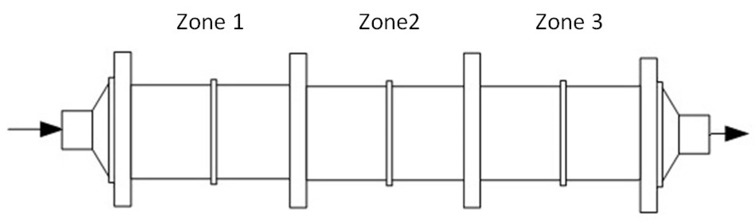
3.2.2. Dispersion Model

A dispersion (diffusion) model is used for to model non-ideal plug-flow reactors and is written in the form of a dimensionless partial differential equation [44]. The main parameter of the dispersion model is the value of the Bodenstein number (Bo). The Bodenstein number, as well as the average particle residence time ($\overline{\tau }$) is usually determined based on the calculation of the probability characteristics of the distribution curve or other methods [45,46,47,48]. The Bodenstein number (Bo) and the Peclet number (Pe) are sometimes used interchangeably in this context, although the numbers have a slightly different meaning [44].

We transform equations of the diffusion model into the criterial form using dependences (1) and (2). The PFR model is used in the simplest case for the tubular reactor, affording $C/{∆}_{\tau }=-\omega ln{S}_C/∆x$; then, $ln{S}_C=1$, where $\omega$ is the flow rate. Similarly, for a one-parameter diffusion model of a tubular reactor:

$$ln{S}_C=\frac{2\omega ∆x}{D_L}=2B{o}_L$$

(30)

For a two-parameter diffusion model:

$$ln{S}_C=\frac{\left(2B{o}_A-ln{S}_A\right)B{o}_L}{B{o}_L+B{o}_A}$$

(31)

where $B{o}_A$ is the Bodenstein number for the case of axial mixing, and $B{o}_L$ is the Bodenstein number for longitudinal mixing.

When $B{o}_L\gg B{o}_R$, Equation (30) takes the form of dependence (31).

To reduce the time required for an experiment to determine the shape of the curve of the distribution function and verify the adequacy of the investigated reactor with the complex model, it is necessary to obtain the values of $\overline{\tau }$, the average residence time, using the time-similarity simplex from (28).

$$ln{S}_c{S}_{\tau }^T=Bo·T^2{{\displaystyle \sum }}_1^2{H}_{0x},$$

(32)

where $T={\tau }_L/\overline{\tau }$ is a constant, ${\tau }_L$ is the flow time along the axis of the tubular reactor, $\overline{\tau }$ is the average residence time, $H_{01}=∆\tau Q/V_0$ is homochronicity number for a flow with perfect mixing, and $H_{02}=∆\tau Q{V}_0/V^2$/V is the homochronicity number for a flow with a dead zone.

For a one-parameter diffusion model of a tubular apparatus, $T=0.5$.

$$ln{S}_n{S}_{\tau }^{0,5}=Bo·{0.5}^{2}Ho-\frac{{(S_r-1)}^2}{Ho{S}_{\tau }},$$

(33)

$$ln{S}_c{S}_{\tau }^{0,5}=\frac{Bo∆\tau }{4\overline{\tau }}\left(1-\frac{{\overline{\tau }}^2}{{\tau }_i ·{\tau }_{i+1}}\right),$$

(34)

or

$$ln{S}_c{S}_{\tau }^{0,5}=A-B\left(\frac{1}{{\tau }_i ·{\tau }_{i+1}}\right)$$

(35)

where A and B are constant value, and $A=\frac{Bo∆\tau }{4\overline{\tau }}, B=\frac{Bo∆\tau }{4}·\overline{\tau }$.

The experimental data on the RTD of coke particles in a tubular rotary kiln in the corresponding coordinate system lie on a straight line. To find the values of $\overline{\tau }$ and Bo, the constants A and B are determined; then, the calculations are carried out according to the following formulae: $\overline{\tau }=\sqrt{B/A}$, $Bo=4\sqrt{A·B}/∆\tau$.

As an example, Figure 3 shows the results of processing the experimental data given in [49]. Experimental data on the RTD of particles in the apparatus are obtained under the condition of a tracer impulse added at the inlet. The RTD of the process can be observed as a tracer concentration profile at the outlet. The data obtained during the experiment should lie on a straight line in the appropriate coordinate system. As shown in Figure 3, the experimental points for two cases are close to a straight line. Their scatter is obviously associated with errors that occurred when determining the indicator concentration at the beginning and end of the experiment, when its value decreased significantly. The difference between the calculated values of the parameters from the data given in [35,49] is less than 2%.

4. Conclusions

Analyzing the simplex-interval equations above, we can conclude that the proposed method can be used to determine the parameters of various technological processes. The type of curves obtained depends on the nature of the kinetic process and the mathematical equation type used to describe it. The considered equations allow for calculation on different intervals. As a result, they can describe both differential and integral dependencies. The simplex-interval method provides calculations of process parameters using a limited number of experimental points. Therefore, simplex-interval dependencies can be widely used in engineering calculations to effectively monitor the progress of an investigated process.

In addition to solving the various problems considered in the present manuscript, the simplices and similarity criteria can be used to carry out a more detailed study of various chemical and metallurgical apparatus operational features with a complex flow structure. Thus, in this work, a new approach is proposed for calculating the operational parameters of various models wherein reactions of the n-th order take place. This approach can represent calculations with the direct use of experimental data without a preliminary determination of the parameters of the kinetic model or the distribution function. The proposed method can be extended to cascade reactors that can be described by a complex tanks-in-series model, particularly when the reaction order differs from the stoichiometric order.

Another topic of interest is that the extension of mathematical models obtained on the basis of the simplex method can serve as the basis for the development of model-predictive controllers.

References

1. Carlson, R.; Carlson, J.E. Design and Optimization in Organic Synthesis: Second Revised and Enlarged Edition; Elsevier Science: Amsterdam, The Netherlands, 2005; ISBN 9780080455273. [Google Scholar]
2. Bonvin, D.; Georgakis, C.; Pantelides, C.C.; Barolo, M.; Grover, M.A.; Rodrigues, D.; Schneider, R.; Dochain, D. Linking Models and Experiments. Ind. Eng. Chem. Res. 2016, 55, 6891–6903. [Google Scholar] [CrossRef]
3. Li, S. Reaction Engineering. In Handbook of Heterogeneous Catalysis; Wiley: Hoboken, NJ, USA, 2017; pp. 1–664. [Google Scholar] [CrossRef]
4. Carr, R.W. Modeling of Chemical Reactions. In Comprehensive Chemical Kinetics; Elsevier: Amsterdam, The Netherlands, 2007; p. 297. [Google Scholar]
5. Bueno, M.P.; Kojovic, T.; Powell, M.S.; Shi, F. Multi-Component AG/SAG Mill Model. Miner. Eng. 2013, 43–44, 12–21. [Google Scholar] [CrossRef]
6. Cameron, I.; Gani, R. Product and Process Modelling; Elsevier: Amsterdam, The Netherlands, 2011; p. 571. [Google Scholar] [CrossRef]
7. Quaglio, M.; Roberts, L.; bin Jaapar, M.S.; Fraga, E.S.; Dua, V.; Galvanin, F. An Artificial Neural Network Approach to Recognise Kinetic Models from Experimental Data. Comput. Chem. Eng. 2020, 135, 106759. [Google Scholar] [CrossRef]
8. Zhang, L.; Li, L.; Wang, S.; Zhu, B. Optimization of LPDC Process Parameters Using the Combination of Artificial Neural Network and Genetic Algorithm Method. J. Mater. Eng. Perform. 2012, 21, 492–499. [Google Scholar] [CrossRef]
9. Chi, C.; Janiga, G.; Thévenin, D. On-the-Fly Artificial Neural Network for Chemical Kinetics in Direct Numerical Simulations of Premixed Combustion. Combust. Flame 2021, 226, 467–477. [Google Scholar] [CrossRef]
10. Nelder, J.A.; Mead, R. A Simplex Method for Function Minimization. Comput. J. 1965, 7, 308–313. [Google Scholar] [CrossRef]
11. Morgan, S.L.; Deming, S.N. Simplex Optimization of Analytical Chemical Methods. Anal. Chem. 1974, 46, 1170–1181. [Google Scholar] [CrossRef]
12. Olsson, D.M.; Nelson, L.S. The Nelder-Mead Simplex Procedure for Function Minimization. Technometrics 1975, 17, 45–51. [Google Scholar] [CrossRef]
13. Spendley, W.; Hext, G.R.; Himsworth, F.R. Sequential Application of Simplex Designs in Optimisation and Evolutionary Operation. Technometrics 1962, 4, 441. [Google Scholar] [CrossRef]
14. Li, H.; Nalim, R.; Haldi, P.A. Thermal-Economic Optimization of a Distributed Multi-Generation Energy System—A Case Study of Beijing. Appl. Therm. Eng. 2006, 26, 709–719. [Google Scholar] [CrossRef]
15. Hu, H.; Zhu, Y.; Peng, H.; Ding, G.; Sun, S. Effect of Tube Diameter on Pressure Drop Characteristics of Refrigerant-Oil Mixture Flow Boiling inside Metal-Foam Filled Tubes. Appl. Therm. Eng. 2013, 61, 433–443. [Google Scholar] [CrossRef]
16. Wang, J.J.; Jing, Y.Y.; Zhang, C.F. Optimization of Capacity and Operation for CCHP System by Genetic Algorithm. Appl. Energy 2010, 87, 1325–1335. [Google Scholar] [CrossRef]
17. Fan, S.K.S.; Liang, Y.C.; Zahara, E. A Genetic Algorithm and a Particle Swarm Optimizer Hybridized with Nelder–Mead Simplex Search. Comput. Ind. Eng. 2006, 50, 401–425. [Google Scholar] [CrossRef]
18. Lin, H.; Yamashita, K. Hybrid Simplex Genetic Algorithm for Blind Equalization Using RBF Networks. Math. Comput. Simul. 2002, 59, 293–304. [Google Scholar] [CrossRef]
19. Li, S.; Xin, F.; Li, L. Fluidized Bed Reactor. In Reaction Engineering; Elsevier: Amsterdam, The Netherlands, 2017; pp. 369–403. [Google Scholar]
20. Burton, K.W.C.; Nickless, G. Optimisation via Simplex. Part I. Background, Definitions and a Simple Application. Chemom. Intell. Lab. Syst. 1987, 1, 135–149. [Google Scholar] [CrossRef]
21. Liotta, F.; Chatellier, P.; Esposito, G.; Fabbricino, M.; Van Hullebusch, E.D.; Lens, P.N.L. Hydrodynamic Mathematical Modelling of Aerobic Plug Flow and Nonideal Flow Reactors: A Critical and Historical Review. Crit. Rev. Environ. Sci. Technol. 2014, 44, 2642–2673. [Google Scholar] [CrossRef]
22. Toson, P.; Doshi, P.; Jajcevic, D. Explicit Residence Time Distribution of a Generalised Cascade of Continuous Stirred Tank Reactors for a Description of Short Recirculation Time (Bypassing). Processes 2019, 7, 615. [Google Scholar] [CrossRef]
23. Gorzalski, A.S.; Harrington, G.W.; Coronell, O. Modeling Water Treatment Reactor Hydraulics Using Reactor Networks. J. Am. Water Work. Assoc. 2018, 110, 13–29. [Google Scholar] [CrossRef]
24. Sheoran, M.; Chandra, A.; Bhunia, H.; Bajpai, P.K.; Pant, H.J. Residence time distribution studies using radiotracers in chemical industry—A review. Chem. Eng. Commun. 2018, 205, 739–758. [Google Scholar] [CrossRef]
25. Vyazovkin, S.V.; Goryachko, V.I.; Lesnikovich, A.I. An Approach to the Solution of the Inverse Kinetic Problem in the Case of Complex Processes. Part III. Parallel Independent Reactions. Thermochim. Acta 1992, 197, 41–51. [Google Scholar] [CrossRef]
26. Braun, R.L.; Burnham, A.K. Analysis of Chemical Reaction Kinetics Using a Distribution of Activation Energies and Simpler Models. Energy Fuels 1987, 1, 153–161. [Google Scholar] [CrossRef]
27. Levin, V.I. Optimization in terms of interval uncertainty: The determinization method. Autom. Control. Comput. Sci. 2012, 46, 157–163. [Google Scholar] [CrossRef]
28. Gorlanov, E.S.; Brichkin, V.N. Polyakov Electrolytic production of aluminium: Review. part 1. conventional areas of development. Tsvetnye Met. 2020, 2, 36–41. [Google Scholar] [CrossRef]
29. Savchenkov, S.A.; Bazhin, V.Y.; Brichkin, V.N.; Povarov, V.G.; Ugolkov, V.L.; Kasymova, D.R. Synthesis of magnesium-zinc-yttrium master alloy. Lett. Mater. 2019, 9, 339–343. [Google Scholar] [CrossRef]
30. Savchenkov, S.A.; Bazhin, V.Y.; Brichkin, V.N.; Kosov, Y.I.; Ugolkov, V.L. Production Features of Magnesium-Neodymium Master Alloy Synthesis. Metallurgist 2019, 63, 394–402. [Google Scholar] [CrossRef]
31. Cleary, P.W.; Monaghan, J.J. Conduction Modelling Using Smoothed Particle Hydrodynamics. J. Comput. Phys. 1999, 148, 227–264. [Google Scholar] [CrossRef]
32. Kondrasheva, N.K.; Rudko, V.A.; Ancheyta, J. Thermogravimetric Determination of the Kinetics of Petroleum Needle Coke Formation by Decantoil Thermolysis. ACS Omega 2020, 5, 29570–29576. [Google Scholar] [CrossRef]
33. Beloglazov, I.N.; Beloglazov, N.K. The Simplex Method to Describe Hydrometallurgical Processes. Miner. Process. Extr. Metall. Rev. 1995, 15, 139. [Google Scholar] [CrossRef]
34. Smol’nikov, A.D.; Sharikov, Y.V. Simulation of the Aluminum Electrolysis Process in a High-Current Electrolytic Cell in Modern Software. Metallurgist 2020, 63, 1313–1320. [Google Scholar] [CrossRef]
35. Sharikov, F.Y.; Sharikov, Y.V.; Krylov, K.A. Selection of key parameters for green coke calcination in a tubular rotary kiln to produce anode petcoke. ARPN J. Eng. Appl. Sci. 2020, 15, 2904–2912. [Google Scholar]
36. Cheremisina, O.V.; Cheremisina, E.A.; Ponomareva, M.A.; Fedorov, A.T. Sorption of rare earth coordination compounds. J. Min. Inst. 2020, 244, 474–481. [Google Scholar] [CrossRef]
37. Cheremisina, E.; Cheremisina, O.; Ponomareva, M.; Bolotov, V.; Fedorov, A. Kinetic Features of the Hydrogen Sulfide Sorption on the Ferro-Manganese Material. Metals 2021, 11, 90. [Google Scholar] [CrossRef]
38. Kondrasheva, N.K.; Rudko, V.A.; Nazarenko, M.Y.; Gabdulkhakov, R.R. Influence of parameters of delayed asphalt coking process on yield and quality of liquid and solid-phase products. J. Min. Inst. 2020, 241, 97. [Google Scholar] [CrossRef]
39. Rehrl, J.; Kruisz, J.; Sacher, S.; Khinast, J.; Horn, M. Optimized continuous pharmaceutical manufacturing via model-predictive control. Int. J. Pharm. 2016, 510, 100–115. [Google Scholar] [CrossRef] [PubMed]
40. Tsai, H.-H.; Fuh, C.-C.; Ho, J.-R.; Lin, C.-K. Design of Optimal Controllers for Unknown Dynamic Systems through the Nelder–Mead Simplex Method. Mathematics 2021, 9, 2013. [Google Scholar] [CrossRef]
41. Visuthirattanamanee, R.; Sinapiromsaran, K.; Boonperm, A. Self-Regulating Artificial-Free Linear Programming Solver Using a Jump and Simplex Method. Mathematics 2020, 8, 356. [Google Scholar] [CrossRef]
42. Gutierrez, C.G.C.C.; Dias, E.F.T.S.; Gut, J.A.W. Residence time distribution in holding tubes using generalized convection model and numerical convolution for non-ideal tracer detection. J. Food Eng. 2010, 98, 248–256. [Google Scholar] [CrossRef]
43. Islamov, S.R.; Bondarenko, A.V.; Mardashov, D.V. Substantiation of a Well Killing Technology for Fractured Carbonate Reservoirs. In Youth Technical Sessions Proceedings; CRC Press: Boca Raton, FL, USA, 2019; pp. 256–264. [Google Scholar] [CrossRef]
44. Levenspiel, O.; Smith, W.K. Notes on the diffusion-type model for the longitudinal mixing of fluids in flow. Chem. Eng. Sci. 1957, 6, 227–235. [Google Scholar] [CrossRef]
45. Dittrich, E.; Klincsik, M. Analysis of conservative tracer measurement results using the Frechet distribution at planted horizontal subsurface flow constructed wetlands filled with coarse gravel and showing the effect of clogging processes. Environ. Sci. Pollut. Res. 2015, 22, 17104–17122. [Google Scholar] [CrossRef]
46. Braga, B.M.; Tavares, R.P. Description of a New Tundish Model for Treating RTD Data and Discussion of the Communication “New Insight into Combined Model and Revised Model for RTD Curves in a Multi-strand Tundish” by Lei. Met. Mater. Trans. A 2018, 49, 2128–2132. [Google Scholar] [CrossRef]
47. Dryer, F.L.; Haas, F.M.; Santner, J.; Farouk, T.I.; Chaos, M. Interpreting chemical kinetics from complex reaction–advection–diffusion systems: Modeling of flow reactors and related experiments. Prog. Energy Combust. Sci. 2014, 44, 19–39. [Google Scholar] [CrossRef]
48. Shestakov, A.K.; Sadykov, R.M.; Petrov, P.A. Multifunctional crust breaker for automatic alumina feeding system of aluminum reduction cell. E3S Web Conf. 2021, 266, 09002. [Google Scholar] [CrossRef]
49. Sharikov, Y.V.; Sharikov, F.Y.; Krylov, K.A. Mathematical Model of Optimum Control for Petroleum Coke Production in a Rotary Tube Kiln. Theor. Found. Chem. Eng. 2021, 55, 711–719. [Google Scholar] [CrossRef]
Figure 1. CSTR in-series model for a tubular rotary kiln.
Mathematics 10 02959 g001
Figure 2. The dependence of lnSc = φ(lnSτ) for a cascade of perfect mixing reactors.
Mathematics 10 02959 g002
Figure 3. The dependence of l n S c = φ ( 1 / τ i   · τ i + 1 ) for the dispersion model for two experimental data points (a,b).
Mathematics 10 02959 g003