Day-Ahead Scheduling of On-Load Tap Changer Transformer and Switched Capacitors by Multi-Pareto Optimality

Abstract

In this study, a multi-objective optimization method is proposed to solve day-ahead voltage control problems in distribution systems. The main purpose is to determine the optimal schedule for on-load tap changer (OLTC) settings at the sub-station and switched capacitors (SC) based on day-ahead load forecasting. The optimization criteria presented in this study include: (1) minimizing the voltage deviations at the main transformer bus, and (2) minimizing the total power loss. In the proposed method, the Pareto front and Manhattan distance are combined as indices to assess and select the best solution. Multi-Pareto optimality is used to improve the performance of the proposed scheduling strategy. In this study, the network components were modeled by the DIgSILENT Power Factory 15.2, while the multi-objective optimization algorithm was implemented on the MATLAB 2016a software package. Additionally, the effects of different distributed generation (DG) grid-connected points and operation scenarios on voltage control scheduling were examined. The efficiency and performance of the proposed method were verified using an IEEE 33 BUS test system. Compared with the local voltage level (LVL) and reactive power device control (RPDC) methods, the proposed method delivered percentage reductions in (1) voltage deviations at all buses, (2) voltage variations, (3) total system power loss, and (4) difference in values of up to 160.93%, 31.16%, 10.35%, and 434.34%, respectively.

1. Introduction

1.1. Background

In recent years, owing to the rise in environmental awareness and the growing challenges of global energy supply, governments are actively developing policies worldwide for power generation from renewable energy sources. The installed capacity of renewable energy increased rapidly, with solar and wind energy infrastructure constituting a majority of the total capacity. The Renewables 2020 Global Status Report indicates that the installed capacity of renewable energy increased by more than 200 GW, with solar energy accounting for the largest proportion. Compared to 2018, the global investment funds for renewable energy in 2019 grew by 2%. Since 2009, funds invested in wind power surpassed those invested in solar power. Information reports show that renewable energy plays an important role in power generation, and thus cannot be ignored. Renewable energy infrastructure is still being developed. Renewable Capacity Statistics 2021 indicates that the total installed capacity of global solar energy generation reached 713 GW in 2020, which is nearly ten times higher than that in 2011 (73 GW) [1]. The total installed capacity of global wind power generation reached 733 GW, which is three times higher than that in 2011. The report also pointed out that the installed capacity of global renewable energy increased from 25.1% in 2011 to 36.6% in 2020 [1].

Generally, in radial distribution systems, power is transmitted from the upstream power generation side to the downstream load side. Owing to long-range power transmissions and high R/X ratios, the voltage level at the load end fluctuates or decreases. However, with a proper control strategy, installations of distributed generations (DGs) may prove to mitigate the voltage issues to a satisfying level. In contrast, integrating a large number of DGs and distributed energy resources (DERs) into the grid may lead to various directions of power flow, and thus cause changes in voltage spread [2].

Voltage regulation became crucial for the secure and safe operation of a power system. Traditionally, on-load tap changer (OLTC) transformers or switched capacitors (SCs) are often used in voltage control systems [3]. The most common control structure is the decentralized control system, which handles the local voltages and local information. The implementation of such a control system is easy, as well as cost-effective. Another popular control structure handles the entire system and is known as the centralized control system [4]. The entire system information is used to stabilize the voltage profile. However, it fails to adapt to the increasing number of DGs. Recently, another approach for a hybrid control structure is implemented, which takes up the advantages of both systems [5]. However, implementation of such a system is expensive and complex. Several other methods, including local voltage level (LVL), line drop compensation (LDC), step voltage regulators, and reactive power device control (RPDC) are used for voltage control of the feeders, as discussed in the literature review section. However, the integration of DG into the power grid and the increase in power generation using renewable energy sources resulted in additional voltage control problems.

1.2. Aim and Contribution

Based on the above studies, it is seen that scheduling problems are difficult to solve effectively. In this study, a search strategy multi-objective MOPSO method combined with multi-Pareto fronts is proposed to determine the optimal schedule for switching operations for OLTC transformers and SCs over a day, as well as to minimize the voltage deviations of all feeders and total power loss. The proposed method was verified using the IEEE 33 bus system in the presence of a DG. The proposed method was compared with similar optimization algorithms, such as genetic algorithm (GA), PSO, binary ant colony (BAC), and similar voltage control methods, such as LVL and RPDC. In this study, the network components were modeled using DIgSILENT Power Factory 15.2, while the multi-objective optimization algorithm was implemented using MATLAB 2016a. The data exchange process was carried out by using two buffer files, as shown in Figure 1.

1.3. Paper Organization

The remainder of this paper is organized into six sections as follows: Section 2 discusses the related studies; Section 3 formulates the problem and explains the objective functions and constraints; Section 4 describes the multi-objective optimization method and Section 5 explains the proposed day-ahead scheduling method, while Section 6 presents the results and discussion, followed by the conclusion.

2. Related Studies

In recent years, many researchers proposed solutions for optimal voltage control, mainly aiming to mitigate voltage deviation and system power loss. Table 1 depicts some recent publications with their objectives and limitations. Voltage regulators and controllers are broadly divided into discrete controllers (i.e., OLTC and SCs) and continuous controllers (i.e., DERs and DGs). In [6], a local network-based control strategy was proposed for DG. A linear approximation of AC flow power was used to determine the individual characteristics of the DG, thereby improving the voltage profile. Similarly, in [7], an optimal set-point design for voltage and reactive power was established and later solved using optimization algorithms. The inverter-based DG injects or absorbs reactive power that regulates voltage fluctuations in the power system. Similarly, a reactive power controller was proposed using a coordinated scheme between the capacitor banks and DG through remote terminal unit (RTU) data [8]. In [9], a multi-objective evolutionary optimization method was used to model a volt/var compensator. A multiagent control (MAC) system for distribution systems was proposed in [10,11]. A decentralized control structure was used in [12] for reactive power control and monitoring. However, it fails to achieve efficiency, owing to low communication among sub-systems. In [13,14], LVL control strategy was used to regulate the voltage profile of feeders. In another study [15], a stable voltage profile was achieved by incorporating centralized controller. The model predictive control method was adopted to optimize the control environment. Coordinated control between the DG and voltage devices was introduced in [16]. A data structure-based control was proposed in [17], which divided the entire distribution system into several sections via an optimized controller. The coordination was established between the power grid-connected inverter and the distribution static synchronous compensator (D-STATCOM) to control the power flows at the desirable levels. However, real-time operation of power systems is difficult and complex.

Despite the aforementioned studies, the conventional OLTC/SCs-based voltage control method is prevalent in most power grids worldwide. The installation of other voltage control systems is complex and costly. In [18], a distributed control system with OLTC transformers is installed in a distribution system. However, the day-to-day load changes in feeders and the installations of DGs were not considered. In [19], additional control for the reactive power of DGs was extended. In a subsequent study [20], a reactive power controller was modeled in order to control the voltage profile of the system using the least number of tap positions in a PV-dominated distribution system. Furthermore, [21,22] focused on evaluating the LDC of OLTC transformers in accordance with load changes and DG fluctuations. Day-ahead scheduling of SCs, OLTC transformers, and states of DGs inverters are provided in [23]. A scheduling technique was developed in [24] with the least number of capacitor switch operations to minimize the cost of operation and improve the voltage profile. Furthermore, a mixed integer linear programming (MILP) model was developed for the volt–var problem converted into a nonlinear optimization case [25]. Similarly, the volt–var optimizing problem was solved using fuzzy logic systems [26]. However, because the switching cost is considerably high and numerous variables must be considered, determining the optimal daily operating schedules for OLTC transformers and SCs is a complex problem.

In [27], a particle swarm optimization (PSO) algorithm was incorporated with evolutionary and dynamic programming to solve the optimization problem. However, the issue of local optima cannot be avoided in high-dimensional scenarios. This drawback was neutralized using the multi-objective PSO (MOPSO) concept. In recent years, MOPSO was successfully used in the applications of measurement, [28], image processing [29], renewable energy systems [30], and chemistry [31].

Table 1. Contributions and Drawbacks of related studies.

References	Natures	Contributions	Drawbacks
Refs. [6,7]	Complex	Real-time voltage control method proposed using a linear approximation of ac power flow.	Local controller utilized lacking overall network stability.
Ref. [8]	Complex, coordinated	Voltage control through reactive power control using coordination between DGs and capacitor banks.	Demands expensive communication structures among local and central systems.
Ref. [9]	Very complex	A volt–var compensator proposed using coordinated control proposed with evolutionary optimization.	Unable to derive strategies for multi-energy microgrid scenarios.
Refs. [10,11]	Complex	A multi-agent system (MAS) is proposed to control the reactive power sources in a distribution system.	The communication among the multi-agents is even more complex than normal controllers and increases transition time.
Refs. [13,14]	Simple	Harmonic balance method proposed for voltage controllers using Q(V) control.	Two-end data are needed. Additionally, it cannot reflect the nature of large systems.
Ref. [15]	Complex	Model predictive controller (MPC) is used for coordinated control among the DGs and other voltage controllers.	Implementation of MPC is challenging and has high computation requirements and fine-tuned parameters.
Ref. [16]	Complex	Dynamic programming is used to establish a connection among DGs and OLTC with minimum switch operation.	Reliability depends on the quality of the communication system. PV power sources are not considered.
Ref. [19]	Complex	Cooperative controller is proposed for voltage control involving multiple feeders, loads, and DGs.	Suffers in the presence of microgrids and requires high communication bandwidth.
Ref. [21]	Very simple	Line drop compensator parameters are designed based on the current state of voltage regulators in presence of DG.	Only the OLTC control is considered, which reduces the effectiveness of the voltage regulation method.
Ref. [22]	Complex	Parameters of OLTC are designed in accordance with DG output in order to maintain the voltage profile.	Requires costly widespread communication facility.
Ref. [25]	Simple	Mixed integer non-linear programming (MILP) is used for volt–var control using capacitor banks and DGs.	MILP fails to address high-dimensional problems. Additionally, non-linear cases cannot be handled.
Ref. [26]	Very complex	Proper control parameters of volt–var compensators are obtained while keeping the voltage profiles at the desired range.	A coordinated complex control structure considers OLTC, voltage regulators, and capacitor banks at feeders and sub-stations. Difficulty in practical implementations.
Ref. [27]	Simple	Particle swarm optimization along with dynamic programming is used in solving reactive power control problems.	High-dimensional problems may face the local optima conditions.

Table 1. Contributions and Drawbacks of related studies.

References	Natures	Contributions	Drawbacks
Refs. [6,7]	Complex	Real-time voltage control method proposed using a linear approximation of ac power flow.	Local controller utilized lacking overall network stability.
Ref. [8]	Complex, coordinated	Voltage control through reactive power control using coordination between DGs and capacitor banks.	Demands expensive communication structures among local and central systems.
Ref. [9]	Very complex	A volt–var compensator proposed using coordinated control proposed with evolutionary optimization.	Unable to derive strategies for multi-energy microgrid scenarios.
Refs. [10,11]	Complex	A multi-agent system (MAS) is proposed to control the reactive power sources in a distribution system.	The communication among the multi-agents is even more complex than normal controllers and increases transition time.
Refs. [13,14]	Simple	Harmonic balance method proposed for voltage controllers using Q(V) control.	Two-end data are needed. Additionally, it cannot reflect the nature of large systems.
Ref. [15]	Complex	Model predictive controller (MPC) is used for coordinated control among the DGs and other voltage controllers.	Implementation of MPC is challenging and has high computation requirements and fine-tuned parameters.
Ref. [16]	Complex	Dynamic programming is used to establish a connection among DGs and OLTC with minimum switch operation.	Reliability depends on the quality of the communication system. PV power sources are not considered.
Ref. [19]	Complex	Cooperative controller is proposed for voltage control involving multiple feeders, loads, and DGs.	Suffers in the presence of microgrids and requires high communication bandwidth.
Ref. [21]	Very simple	Line drop compensator parameters are designed based on the current state of voltage regulators in presence of DG.	Only the OLTC control is considered, which reduces the effectiveness of the voltage regulation method.
Ref. [22]	Complex	Parameters of OLTC are designed in accordance with DG output in order to maintain the voltage profile.	Requires costly widespread communication facility.
Ref. [25]	Simple	Mixed integer non-linear programming (MILP) is used for volt–var control using capacitor banks and DGs.	MILP fails to address high-dimensional problems. Additionally, non-linear cases cannot be handled.
Ref. [26]	Very complex	Proper control parameters of volt–var compensators are obtained while keeping the voltage profiles at the desired range.	A coordinated complex control structure considers OLTC, voltage regulators, and capacitor banks at feeders and sub-stations. Difficulty in practical implementations.
Ref. [27]	Simple	Particle swarm optimization along with dynamic programming is used in solving reactive power control problems.	High-dimensional problems may face the local optima conditions.

3. Problem Formulation

In distribution systems, OLTC transformers and SCs are typically used to compensate for the voltage drops of transformers and downstream feeders. In the proposed voltage control method, the voltage deviation of the feeders, total power loss, schedule of switching operations for the OLTC transformer, and SCs were considered over the course of a day.

The multi-objective problem can be defined through (1) objective function, (2) inequality restriction, and (3) feasible solution region:

$$\min f_n\left(\mathit{x},\mathit{u}\right), n\in \left\{1,2,\cdots ,N\right\}$$

(1)

subject to,

$$g_j\left(\mathit{x},\mathit{u}\right)\le 0,\begin{array}{cc}& j\in \left\{1,2,\cdots ,J\right\}\end{array}$$

(2)

$$\mathit{x}\in \mathit{X}$$

(3)

where $f_n\left(\mathit{x},\mathit{u}\right)$ is the nth objective function, $g_j\left(\mathit{x},\mathit{u}\right)$ is the jth inequality constraint, $\mathit{x}$ is the variable vector, $\mathit{u}$ is the dependent variable vector, $N$ is the total number of objective functions, $J$ is the total number of inequality constraints, and $\mathit{X}$ is the feasible solution region.

For a distribution system with several buses, the variable vector $\mathit{u}$ includes the bus voltages and power losses of the line segments, which can be expressed as:

$$\mathit{u}={\left[V_1,\dots ,V_n,P_{Loss,1},\dots ,P_{Loss,k}\right]}^t$$

(4)

where $V_n$ is the nth bus voltage in per-unit (pu) and $P_{loss,k}$ is the power loss of the kth line segment in kW.

Based on the MOPSO algorithm, the one-day scheduling of switching operations for the OLTC transformer and SCs can be expressed as $\mathit{x}$ in:

$$\mathit{x}={\left[OLT{C}_1,\cdots ,OLT{C}_j,S{C}_1,\cdots ,S{C}_r\right]}^t$$

(5)

where $OLT{C}_j$ is the tap position of the jth OLTC transformer and $S{C}_r$ is the state of the rth capacitor.

3.1. Objective Functions

Issues concerning load variation situations, maintaining the desired voltages at all buses, and reducing system power loss are very complex. In this study, the following three optimization criteria were considered: (1) voltage deviations at the secondary side of the main transformer, (2) total system power losses, and (3) voltage deviations at the ends of the feeders.

3.1.1. Voltage Deviation at the Secondary Side of the Main Transformer

The first objective is to minimize the voltage deviations on the secondary side of the main transformer, as expressed in:

$$f_1={\sum }_{h=1}^{24}\left|V_s^h-V_r\right| (\mathrm{pu})$$

(6)

where $V_s^h$ indicates the voltage magnitude on the secondary side of the main transformer at the hth hour in pu and $V_r$ represents the desired voltage in pu, which was set at 1.0 pu in this study.

3.1.2. Voltage Deviation at the Ends of the Feeders

The second objective is to minimize the voltage deviation at the end of the feeders, as shown in:

$$f_2={\sum }_{h=1}^{24}\left|V_e^h-V_r\right| (\mathrm{pu})$$

(7)

where $V_e^h$ is the voltage magnitude at the end of the feeder at the hth hour in pu and $V_r$ is the desired voltage in pu, which was set at 1.0 pu in this study.

3.1.3. Total System Power Loss

The third objective is to minimize the total power loss of the power system, as shown in:

$$f_3={\displaystyle \sum }_{h=1}^{24}{P}_{Loss}^h \left(\mathrm{kWh}\right)$$

(8)

where $P_{Loss}^h$ is the total power loss of the feeders at the hth hour in kW.

3.2. Constraints

To maintain the voltage profile along the feeders under desired conditions, operational constraints should be considered, including (1) the operating range of bus voltages, (2) maximum allowable number of switching operations for the OLTC transformer, and (3) maximum allowable number of switching operations for SCs.

3.2.1. Voltage Constraints

All bus voltages were maintained within the designated operating range, as shown in:

$$V_{\min }\le V_N\le V_{\max }$$

(9)

where $V_{\min }$ is the lower limit of bus voltages in pu, which was set at 0.95 pu in this study; $V_{\max }$ is the upper limit of bus voltages in pu, which was set at 1.05 pu in this study; $V_N$ represents the bus voltages at the pilot points in pu, such as the bus voltage at the secondary side of the main transformer, the bus voltage at the end of the feeder, and the bus voltage at the DG grid connection point.

3.2.2. OLTC Transformer Constraints

In engineering, the maintenance cycle or service life of any device depends on its operation conditions. Frequent switching operations for an OLTC transformer may reduce the service life of the transformer or increase its maintenance costs. Therefore, the number of switching operations is restricted within a reasonable range. If the tap position differs from that in the previous hour, a switching operation occurs, as shown in:

$${\displaystyle \sum }_{h=1}^{24}\left(a^h\oplus a^{h-1}\right)\le M$$

(10)

where $a^h$ is the tap position of the OLTC transformer at the hth hour; $\oplus$ is the exclusive OR operation, $a^h\oplus a^{h-1}=1$, as $a^h\ne a^{h-1}$, $a^h\oplus a^{h-1}=0$, as $a^h=a^{h-1}$; and $\mathrm{M}$ represents the maximum allowable number of switching operations for the OLTC transformer.

The number of switching operations of OLTC transformers in the Taiwan Power Company (Taipower) for adjusting the tap position is three over a day (i.e., midnight, daytime, and evening). Therefore, referring to the operating experience of Taipower, the maximum allowable number of switching operations for the transformer tap is three in this study.

3.2.3. SC Constraints

Generally, the maintenance cycle of any device depends on its operation conditions. Frequent switching operations for SCs installed on the secondary side of the main transformer may increase the maintenance costs. Further, the switching operations of SCs may affect those of OLTC transformers. Hence, the maximum allowable number of switching operations for the capacitor is the same as that for the OLTC tap, as shown in:

$${\displaystyle \sum }_{h=1}^{24}\left(C^h\oplus C^{h-1}\right)\le M$$

(11)

where $C^h$ is the on/off state of the SC at the hth hour; $\oplus$ is the exclusive OR operation, $C^h\oplus C^{h-1}=1$, as $C^h\ne C^{h-1}$, $C^h\oplus C^{h-1}=0$, as $C^h=C^{h-1}$; and $\mathrm{M}$ is the maximum allowable number of switching operations for SCs.

4. Multi-Objective Optimization Algorithm

Several methods, including the weighting sum, objective function restriction, and objective programming method, are commonly used to address multi-objective engineering problems. However, these methods are susceptible to human subjectivity, and thus fail to provide an optimal solution for all objectives. The Pareto optimality considers multiple objectives. The Pareto optimal solution, which is a set of feasible solutions rather than a single solution, can be used to search for all the objectives. The solutions in the solution set are not dominated by each other for all objective functions.

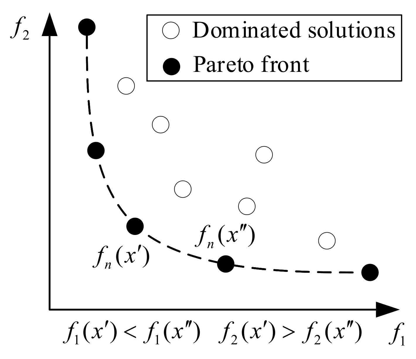
4.1. Pareto Optimality

Pareto optimality does not simplify a multi-objective problem as a single-objective problem; instead, the solutions of the different objective functions are compared individually. A solution is considered Pareto optimal if there exists no other solution that improves the value of any of the objective criteria without deteriorating at least one other criterion. This solution is called a non-dominated or Pareto optimal solution if no other feasible solution dominates. The set of all non-dominated solutions forms the Pareto front, as shown in Figure 2. In terms of minimization objectives, the dominance of the solutions can be expressed as:

$$f_n\left({\mathit{x}}^{\prime }\right)<f_n\left({\mathit{x}}^{″}\right),\begin{array}{cc}& \forall n\in \left\{1,2,\cdots ,N\right\}\end{array}$$

(12)

where ${\mathit{x}}^{\prime }\in \mathit{X}$ and ${\mathit{x}}^{″}\in \mathit{X}$ are the two sets of feasible solutions. The fitness values of ${\mathit{x}}^{\prime }$ for all objectives are better than ${\mathit{x}}^{″}$; therefore, ${\mathit{x}}^{\prime }$ is called the dominant solution, whereas ${\mathit{x}}^{″}$ is the dominated solution, as shown in Figure 3. If there is no possible Pareto improvement, the dominant solution is regarded as a non-dominated solution. The set of all non-dominated solutions in the solution space can be expressed as:

$$\mathit{P}\mathit{S}=\left\{{\mathit{x}}_1,{\mathit{x}}_2,\dots ,{\mathit{x}}_I\right\}$$

(13)

where ${\mathit{x}}_i\in \mathit{X}$ denotes the ith non-dominated solution, and $I$ is the total number of non-dominated solutions.

4.2. MOPSO Algorithm

In multi-objective problems, the objectives to be optimized are generally in conflict with each other. Thus, there is no single solution for these problems. After combining the search ability of the original PSO and the characteristics of Pareto optimality, the MOPSO algorithm [32] was applied to solve multi-objective optimization problems. In the MOPSO calculation process, the non-dominated solutions are stored in a repository, which is called an external archive. In the external archive, any dominant solution can be selected as the global best solution (Gbest) to update velocity and the position of particles.

The external archive plays a key role in improving the searchability of the PSO algorithm. The traditional single-objective PSO algorithm has only a single Gbest; however, in multi-objective optimization, there may be more than one global best solution. In MOPSO, the particle swarm is properly led to fly towards the target by selecting local and global solutions.

A quality function is used to evaluate the quality of all non-dominated solutions stored in the external archive. Through quality evaluation, the appropriate Gbest is selected to update the particles. Moreover, when the external archive is full, the quality function can be used to determine whether the non-dominated solutions are deleted or retained. In general, the crowding distance computation procedure is used to address the aforementioned problems. Compared to traditional PSO algorithms, the issue of local optimum traps can be avoided by combining the MOPSO algorithm and Pareto optimality. A flowchart of the proposed MOPSO algorithm is shown in Figure 4. The steps of the proposed algorithm are as follows:

Step 1

Set the size of populations for particle swarms, the size of the external archive, and other parameters.

Step 2

Generate the position and velocity of each particle randomly.

Step 3

Evaluate the fitness of individual particles and store the first non-dominated solution in the external archive.

Step 4

Select one non-dominated solution as the Gbest from the external archive.

Step 5

Update the velocity and position of the particles using the PSO algorithm.

Step 5

Evaluate the fitness of each particle.

Step 7

Save new non-dominated solutions.

Step 8

Check whether the external archive is full.

Step 9

If the external archive is not full, the new solution is compared with the solutions stored in the external archive. If the new solution dominates any of the solutions in the archive, the dominated solutions are deleted, and the new non-dominated solution is stored.

Step 10

If the external archive is full, one solution in the most crowded hypercube is randomly removed, and the new non-dominated solution is stored.

Figure 4. Flowchart of the proposed MOPSO algorithm.

Figure 4. Flowchart of the proposed MOPSO algorithm.

4.3. Minimum Manhattan Distance Method

The Manhattan distance, as a Euclidean geometric term, is the sum of the absolute differences between two points in the Cartesian coordinate system. In multi-objective optimization problems, the multiple-criteria decision making (MCDM) method is used to select the final solutions from the Pareto front. In the minimum Manhattan distance (MMD) method, a solution with the minimum distance from a normalized ideal vector is selected [33]. The minimum distance from the normalized ideal vector is called the MMD.

$\mathit{P}\mathit{S}$ was obtained using the MOPSO algorithm. The difference between the maximum and minimum values of each objective function was calculated using:

$$L_n=\underset{{\mathit{x}}_i\in \mathit{P}\mathit{S}}{\max }{f}_n\left({\mathit{x}}_i\right)-\underset{{\mathit{x}}_i\in \mathit{P}\mathit{S}}{\min }{f}_n\left({\mathit{x}}_i\right)$$

(14)

where ${\mathit{x}}_i\in \mathit{P}\mathit{S}$ is the ith solution in the set of all feasible solutions.

The minimum value of the objective function is calculated as:

$${\ell }_n=\underset{{\mathit{x}}_i\in \mathit{P}\mathit{S}}{\min }{f}_n\left({\mathit{x}}_i\right)$$

(15)

In the set of all feasible solutions, the minimum sum of distances from the ideal vector ${\mathit{y}}_{opt}$ is denoted by:

$${\mathit{y}}_{opt}={\left[\begin{array}{cccc}\frac{{\ell }_1}{L_1}& \frac{{\ell }_2}{L_2}& \cdots & \frac{{\ell }_N}{L_N}\end{array}\right]}^t$$

(16)

The vector $\mathit{y}\left({\mathit{x}}_i\right)$ of each solution is denoted as:

$$\mathit{y}({\mathit{x}}_i)={\left[\frac{f_1\left({\mathit{x}}_i\right)}{L_1}\frac{f_2\left({\mathit{x}}_i\right)}{L_2}\cdots \frac{f_N\left({\mathit{x}}_i\right)}{L_N}\right]}^t$$

(17)

The minimum Manhattan distance is defined as:

$$M{D}_i=\Vert \mathit{y}\left({\mathit{x}}_i\right)-{\mathit{y}}_{opt}{\Vert }_1$$

(18)

where $\Vert ·{\Vert }_1$ represents the Manhattan norm (also termed 1-norm), i.e., $\Vert \mathit{y}{\Vert }_1={\sum }_{n=1}^N\left|y_n\right|$.

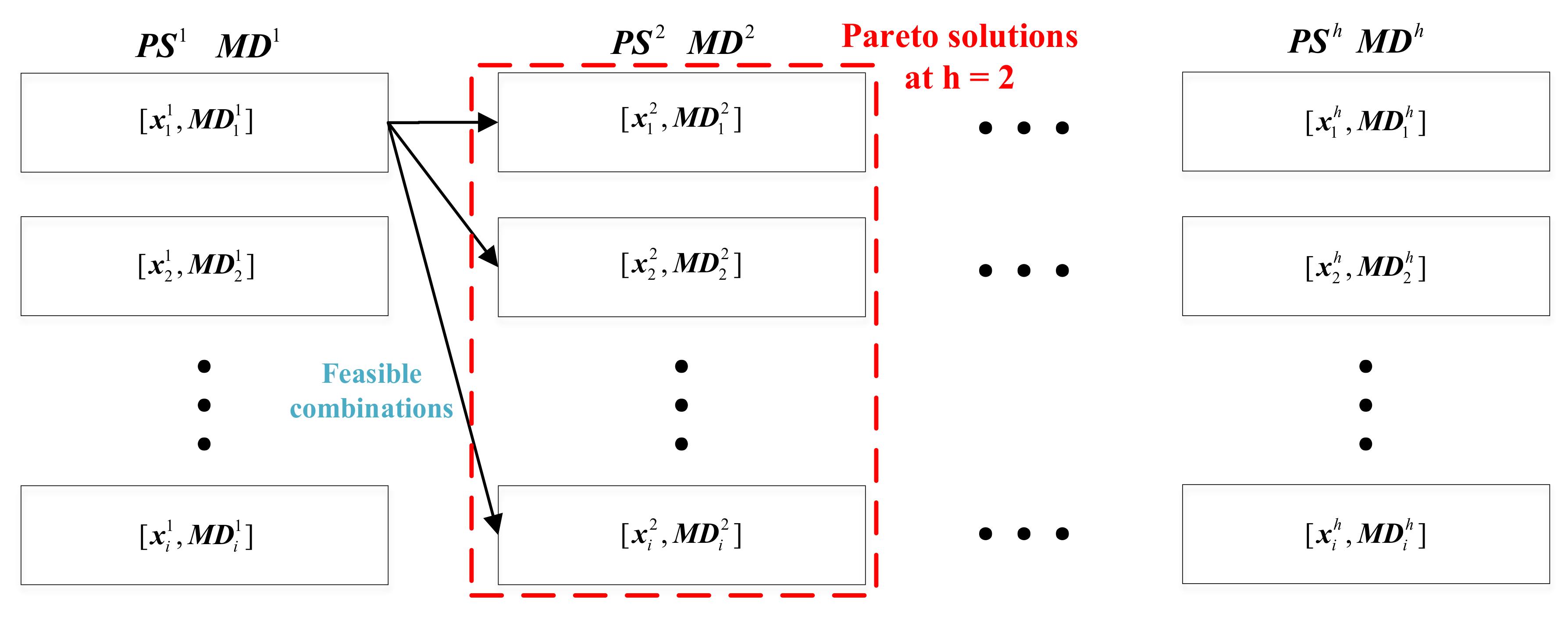
5. One-Day Scheduling Method

Determining the optimal one-day schedule is a complex problem and feasible solutions may not be obtained merely through optimization algorithms. A scheduling strategy that can effectively solve the one-day scheduling problem is proposed in this study. The MOPSO algorithm was used to find per-hour Pareto front solutions. The Manhattan distance method was then used as an index to determine the MMD of a one-day schedule.

The proposed scheduling method is based on day-ahead load forecasting. Based on the hourly load demand and DG, an hourly Pareto front solution can be obtained using the MOPSO algorithm. Multi-Pareto front solutions are more adaptive to individual objective functions for all feasible solutions. With the multi-Pareto front solutions, one-day schedules that satisfy the constraints of switching operations for OLTC transformers and SCs are obtained. The Manhattan distances for the corresponding solutions are summarized, and the schedule with the minimum Manhattan distance is selected as the final solution. A flowchart of the proposed scheduling method is illustrated in Figure 5, and the steps are as follows:

Step 1

Determine hourly Pareto front solutions of the OLTC transformer and SCs using the MOPSO algorithm, as shown in Equation (19).

Step 2

Calculate the distance of the hourly Pareto front solutions using the Manhattan distance method, as shown in Equation (20).

Step 3

Search for feasible one-day schedules that meet the switching constraint of the OLTC transformer as Equation (10) and the switching constraint of SCs as Equation (11) with the hourly Pareto front solutions, as shown in Equation (21).

Step 4

Calculate all possible one-day schedules using Step 3. Calculate the Manhattan distance for one-day schedules by summing the Manhattan distances corresponding to the hourly Pareto solutions, as shown in Equation (24).

Step 5

The schedule with the minimum Manhattan distance is selected from the above feasible solution sets, as shown in Equation (25).

Figure 5. Flowchart of the proposed scheduling method based on the day-ahead DG generation.

Figure 5. Flowchart of the proposed scheduling method based on the day-ahead DG generation.

The MOPSO algorithm was used to calculate the hourly Pareto front solution sets in (19) and the Manhattan distance sets in (20), shown as follows:

$$\mathit{P}{\mathit{S}}^h=\left\{{\mathit{x}}_1^h,{\mathit{x}}_2^h,\dots ,{\mathit{x}}_i^h,\dots \right\} h\in \left\{1,2,\dots ,24\right\}$$

(19)

$$\mathit{M}{\mathit{D}}^h=\left\{M{D}_1^h,M{D}_2^h,\dots ,M{D}_i^h,\dots \right\} h\in \left\{1,2,\dots ,24\right\}$$

(20)

where ${\mathit{x}}_i^h$ is the ith front solution at the hth hour, and $M{D}_i^h$ is the Manhattan distance of the ith front solution at the hth hour.

A schematic of the one-day search schedule is shown in Figure 6. Using the $\mathit{P}{\mathit{S}}^h$ and $\mathit{M}{\mathit{D}}^h$ solutions, the feasible one-day schedules that satisfy the switching constraints of the OLTC transformer and SCs are calculated as:

$$\mathit{T}\mathit{S}=\left\{{\mathit{S}}_1,{\mathit{S}}_2,\dots ,{\mathit{S}}_n,\dots \right\}$$

(21)

The nth set of the scheduling solutions is defined as:

$${\mathit{S}}_n=\left\{{\mathit{x}}_n^1,{\mathit{x}}_n^2,\dots ,{\mathit{x}}_n^h\right\}$$

(22)

The Manhattan distance summation for each hourly scheduling solution set is calculated using:

$$D_n={\displaystyle \sum }_{h=1}^{24}M{D}_n^h$$

(23)

The scheduling solution set for the Manhattan distance summation is defined as:

$$\mathit{T}\mathit{M}\mathit{D}=\left\{D_1,D_2,\dots ,D_n,\dots \right\}$$

(24)

The one-day schedule with minimum Manhattan distance summation is the optimal solution, as shown in:

$$D_{ot}=\min \mathit{T}\mathit{M}\mathit{D}$$

(25)

where ${\mathit{S}}_n$ is the nth solution set of one-day schedules, ${\mathit{x}}_{s,h}$ is the solution at the hth hour, and $M{D}_n^h$ is the Manhattan distance corresponding to the solution at the hth hour.

Figure 6. Schematic of searching one-day schedules with multi-Pareto optimality.

Figure 6. Schematic of searching one-day schedules with multi-Pareto optimality.

6. Sample System and Simulation Results

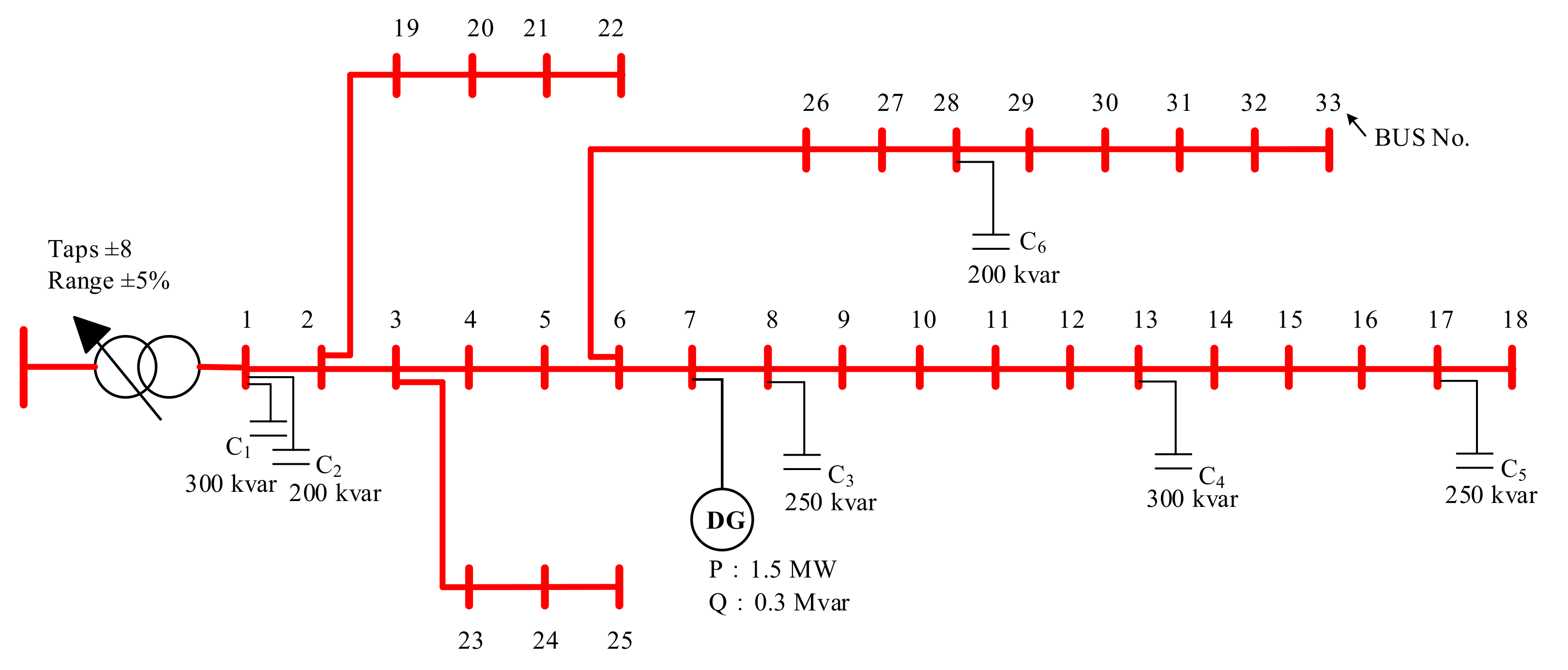
In the simulation, the upper and lower limits of the operating power factor and the extreme voltage variation were considered according to the Taipower Company Renewable Energy Power Generation System Parallel Technology Guidelines. In addition, the effects of different DG grid-connected points and operation scenarios on voltage control scheduling were evaluated. The performance of the proposed voltage control method was compared with those of the LVL [14] and RPDC methods. Finally, the results of the performance of MOPSO and other algorithms were compared and analyzed. The performance of the proposed method was verified using an IEEE 33 bus test system.

6.1. Sample System

The architecture of the sample system is illustrated in Figure 7. Two feeders—feeder A and feeder B—are connected to the secondary side of the main transformer. Feeder A supplies the heavy industrial load demand with a peak of 2.8 MVA. Feeder B supplies a light residential load demand with a peak of 0.4 MVA. The loads at the other feeders are represented as lumped loads on the secondary side of the main transformer with a peak load of 12.17 MVA. The total daily load curves are shown in Figure 8. The OLTC transformers were equipped with ±16 steps of 0.00625 pu each, and the rated capacity of the SCs connected on the secondary side of the main transformer was 3 Mvar. According to the guidelines in Taipower, the power factors for renewable energy power generation should be between 0.9 lagging and 0.95 leading, the maximum wholesale power should be 5 MW, and the voltage deviations should be within ±3%. In this study, the DG power factors, voltage deviations caused by the DGs, and DG locations were considered to determine the allowable DG capacity, and the number of particle swarms was set to 10 and the maximum number of iterations was 70.

Table 2. Parameters of the optimization algorithms.

Parameter	MOPSO	PSO	GA
Number of iterations	70	70	70
Population size	10	10	10
Other related parameters	Cognitive parameter, $c_1=2.0$ Social parameter, $c_2=2.0$	Cognitive parameter, $c_1=2.0$ Social parameter, $c_2=2.0$	Elite count = 2 Crossover fraction = 0.8 Mutation rate = 0.1 Maximum survivalr ate = 2

lists the parameters of the optimization algorithms. The power factors and capacities of the DGs are listed in

Table 3. Simulation cases at different grid-connected points.

Case	DG Location	DG Capacity	Power Factor
Case 01	BUS A3	5.2 MVA	0.95 leading
Case 02		5.2 MVA	0.9 lagging
Case 03	BUS A12	5.2 MVA	0.95 leading
Case 04		1.3 MVA	0.9 lagging
Case 05	BUS B12	5.2 MVA	0.95 leading
Case 06		1.4 MVA	0.9 lagging

.

6.2. Indicators for Validations

Four indicators were used to validate the performance of the voltage control methods: (1) voltage deviations at all buses, (2) voltage variations, (3) total system power loss, and (4) difference in values.

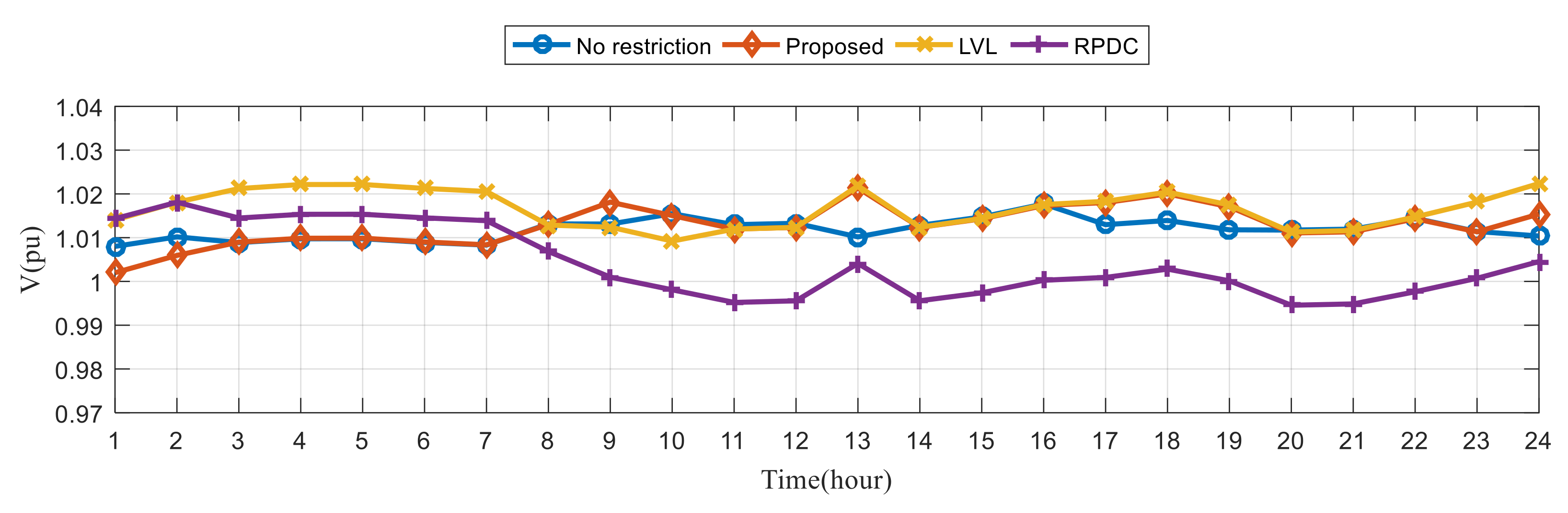
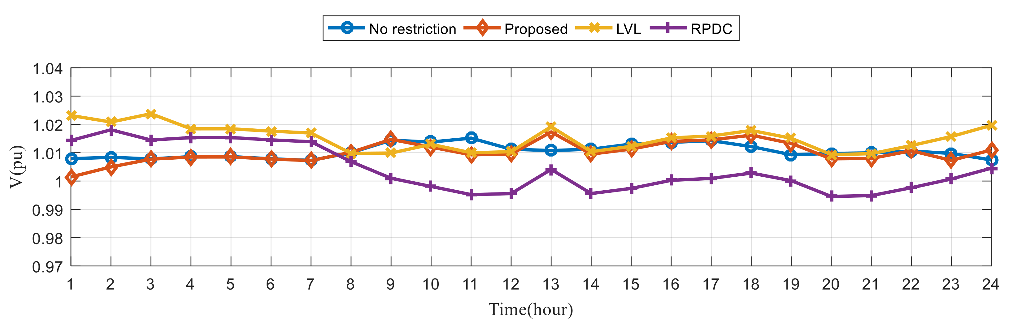
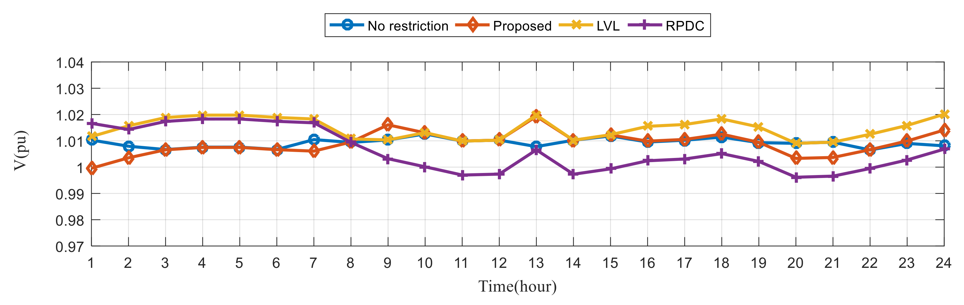
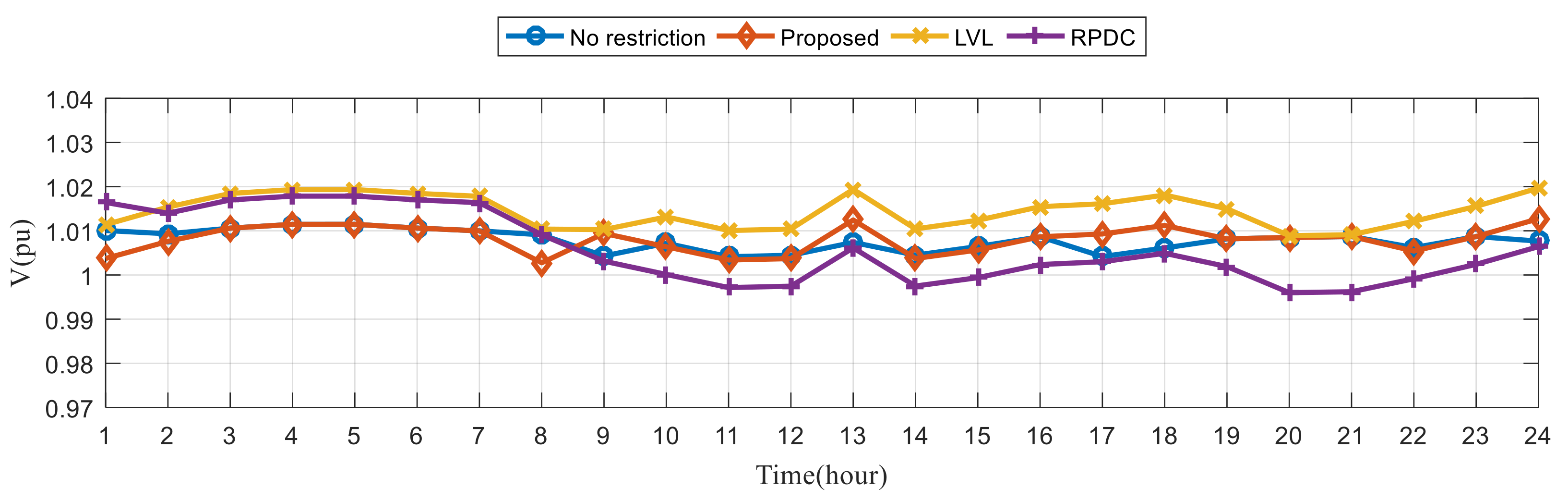
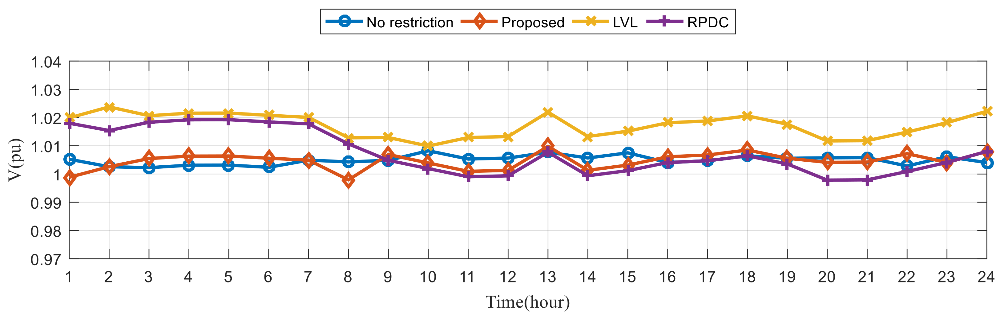
6.2.1. Voltage Deviations at All Buses

The sum of the voltage deviations between all bus voltages and the desired voltages is defined by:

$$G_1={\sum }_{k=1}^n{\sum }_{h=1}^{24}\left|V_k^h-V_r\right| (\mathrm{pu})$$

(26)

where $V_k^h$ is the kth bus voltage at the hth hour; $V_r$ is the desired voltage, which is set to be 1.0 pu in this study; and $n$ is the total number of buses.

6.2.2. Voltage Variations

The sum of the voltage variations between the bus voltages for two successive hours is defined by:

$$G_2={\sum }_k^n{\sum }_{h=1}^{24}\left|V_k^h-V_k^{h-1}\right| (\mathrm{pu})$$

(27)

where $V_k^h$ is the kth bus voltage at the hth hour and $n$ is the total number of buses.

6.2.3. Total System Power Loss

The sum of the real power losses of the feeders is defined by:

$$G_3={\sum }_{h=1}^{24}{P}_{Loss}^h \left(\mathrm{kWh}\right)$$

(28)

where $P_{Loss}^h$ is the power loss of the feeders at the hth hour.

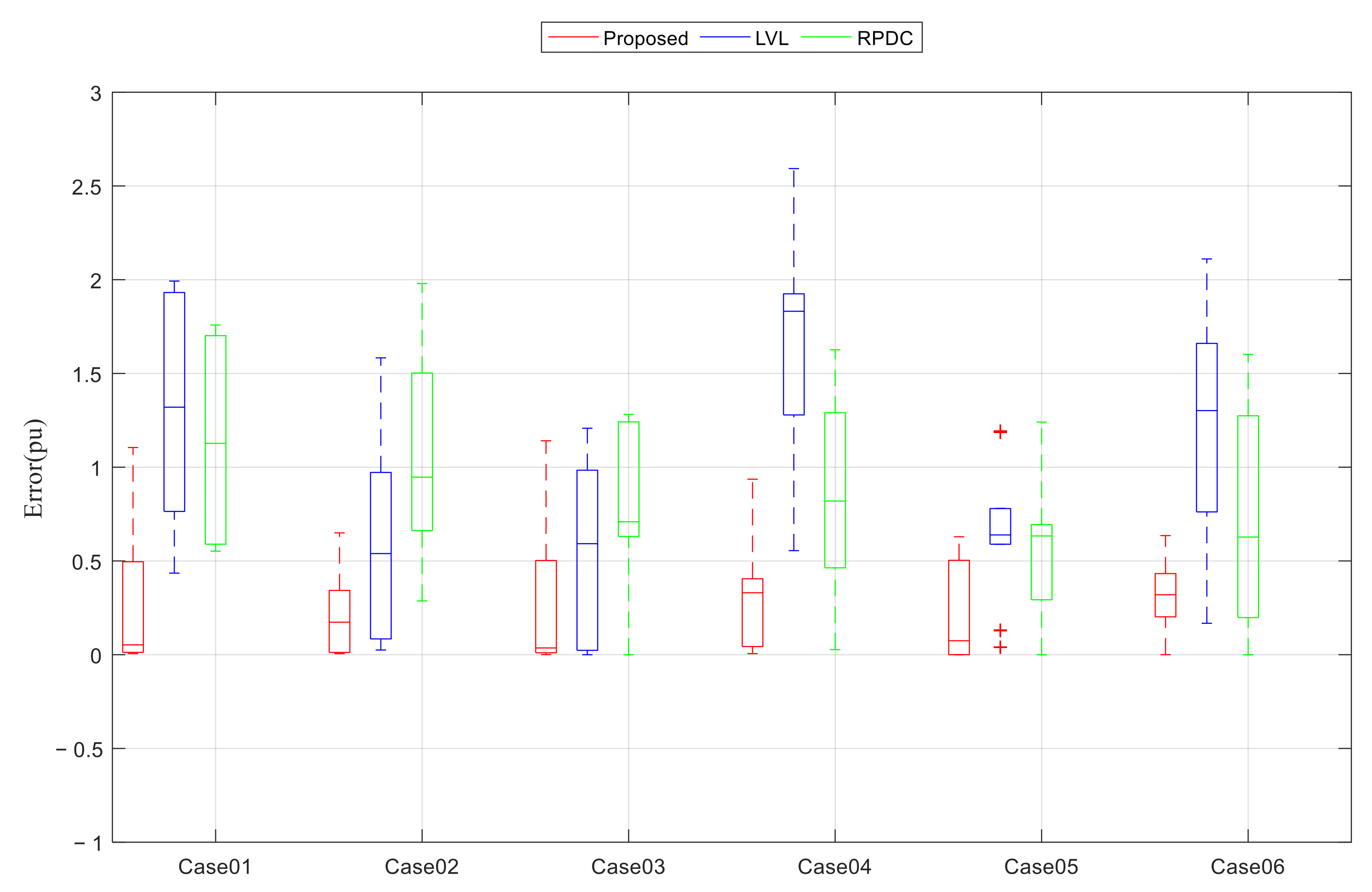
6.2.4. Difference in Values

A schedule without switching restrictions was regarded as the baseline. The difference between the desired voltage value and the voltage after optimal scheduling is calculated as shown in:

$$G_4={\sum }_{h=1}^{24}\left|V_{os}^h-V_{dv}^h\right| (\mathrm{pu})$$

(29)

where $V_{os}^h$ is the voltage at the secondary side of the main transformer at the hth hour after optimal scheduling and $V_{dv}^h$ represents the desired voltage at the secondary side of the main transformer at the hth hour.

6.3. Simulation Results of Sample System

Figure 9 presents the voltage variations of buses A2, A12, and B12, along with the schedule for the OLTC tap position and SCs operation over a day when a DG is connected to bus A3 with 0.95 power factor lagging.

Table 4. Simulation results of the validation indicators for different methods—Case 01.

Method	${\mathit{G}}_1 \left(\mathbf{pu}\right)$	${\mathit{G}}_2 \left(\mathbf{pu}\right)$	${\mathit{G}}_3 \left(\mathbf{MWh}\right)$	${\mathit{G}}_4 \left(\mathbf{pu}\right)$
Proposed method	4.2577	1.6355	0.6848	0.0535
LVL method	6.1747	1.8514	0.6994	0.1347
RPDC method	5.6591	1.9719	0.7144	0.2740

lists the simulation results of the various methods. This shows that the proposed voltage control method outperforms the other voltage control methods because the voltage deviation, voltage variation, and power loss of the proposed method are lower than those of the other methods.

Figure 10, Figure 11, Figure 12, Figure 13, Figure 14 and Figure 15 show that in the different DG scenarios, results of the proposed control method are close to the results obtained by the optimal schedule without switching restrictions, where the proposed method can reduce the switching costs with voltages closer to the desired values as compared to other voltage control methods. The validation indicators for the other simulation cases are presented in Table 4,

Table 5. Simulation results of the validation indicators for different methods—Case 02.

Method	${\mathit{G}}_1 \left(\mathbf{pu}\right)$	${\mathit{G}}_2 \left(\mathbf{pu}\right)$	${\mathit{G}}_3 \left(\mathbf{MWh}\right)$	${\mathit{G}}_4 \left(\mathbf{pu}\right)$
Proposed method	4.03	1.4085	0.4936	0.0488
LVL method	6.5344	1.76	0.5354	0.1400
RPDC method	4.4974	1.8474	0.5447	0.2558

,

Table 6. Simulation results of the validation indicators for different methods—Case 03.

Method	${\mathit{G}}_1 \left(\mathbf{pu}\right)$	${\mathit{G}}_2 \left(\mathbf{pu}\right)$	${\mathit{G}}_3 \left(\mathbf{MWh}\right)$	${\mathit{G}}_4 \left(\mathbf{pu}\right)$
Proposed method	3.0383	1.6599	5.3044	0.0585
LVL method	5.4915	1.8389	5.2394	0.1295
RPDC method	4.5050	1.8929	5.3397	0.2022

,

Table 7. Simulation results of the validation indicators for different methods—Case 04.

Method	${\mathit{G}}_1 \left(\mathbf{pu}\right)$	${\mathit{G}}_2 \left(\mathbf{pu}\right)$	${\mathit{G}}_3 \left(\mathbf{MWh}\right)$	${\mathit{G}}_4 \left(\mathbf{pu}\right)$
Proposed method	3.19	1.925	0.124	0.0725
LVL method	8.3236	1.7831	0.1311	0.3874
RPDC method	4.4348	1.8509	0.1316	0.2074

,

Table 8. Simulation results of the validation indicators for different methods—Case 05.

Method	${\mathit{G}}_1 \left(\mathbf{pu}\right)$	${\mathit{G}}_2 \left(\mathbf{pu}\right)$	${\mathit{G}}_3 \left(\mathbf{MWh}\right)$	${\mathit{G}}_4 \left(\mathbf{pu}\right)$
Proposed method	4.4856	1.6258	6.4291	0.0445
LVL method	6.2075	1.7078	6.352	0.1588
RPDC method	5.283	1.7637	6.4586	0.1350

and

Table 9. Simulation results of the validation indicators for different methods—Case 06.

Method	${\mathit{G}}_1 \left(\mathbf{pu}\right)$	${\mathit{G}}_2 \left(\mathbf{pu}\right)$	${\mathit{G}}_3 \left(\mathbf{MWh}\right)$	${\mathit{G}}_4 \left(\mathbf{pu}\right)$
Proposed method	6.0427	1.6549	0.6645	0.0712
LVL method	9.2652	1.6531	0.655	0.2963
RPDC method	7.426	1.7118	0.6624	0.1664

, respectively. The capacities of the DGs were the same in Cases 01, 03, and 05. It is observed that when a DG unit is connected to bus A12, voltage deviations can be significantly mitigated. However, connecting a DG to the end of the feeder may result in more line loss than connecting a DG to bus A3. On the other hand, connecting a DG to bus A12 fails to mitigate voltage deviations and also has the greatest line loss among the three cases. It is seen that in comparison with the proposed method, other voltage control methods have more voltage deviations and higher switching costs.

Figure 16 shows the box plot (line: median; lower and upper ends of the dotted line: minimum and maximum; lower and upper ends of box: first quartile and third quartile; crosses: outliers) for the hourly voltage deviations of the six cases for the three different voltage control methods. In all cases, the proposed method has much smaller voltage deviations than the other control methods for 75% of the time over 24 h. That is, the voltages of the proposed method are closer to the desired voltages most of the time.

6.4. Performance Test of MOPSO and Other Algorithms

As described in Section 3, the traditional single-objective PSO algorithm has only a single Gbest, whereas MOPSO selects Gbest from the external archive and updates the particles. Hence, under MOPSO, the swarm is not easily trapped in a local optimum, unlike traditional methods, which are more effective in dealing with multi-objective problems. The performances of the proposed MOPSO, PSO, and GA algorithms for solving the scheduling problems are compared by searching for the minimum voltage deviations at buses A2, A12, and B12 from the chosen 12 bus samples without DG interconnection. The test results for the different algorithms after 100 iterations are presented in

Table 10. Test results for 12 buses in the sample system.

Algorithm	Best	Average	Worst	Standard Deviation
MOPSO	0.4847	0.48502	0.4887	3.8010 × 10−5
PSO	0.4847	0.48698	0.5066	9.9358 × 10−4
GA	0.4847	0.48768	0.4934	2.2354 × 10−4

. It can be seen that although all three algorithms obtain a fitness of 0.4847 in terms of the best, GA performs poorly in average iterations, and PSO is trapped in the local optimum and thus obtains a fitness of 0.5066 as the worst. The results show that the proposed MOPSO algorithm avoids the problem of trapping in the local optimum, has better search ability, and can thus be used to solve scheduling problems more effectively.

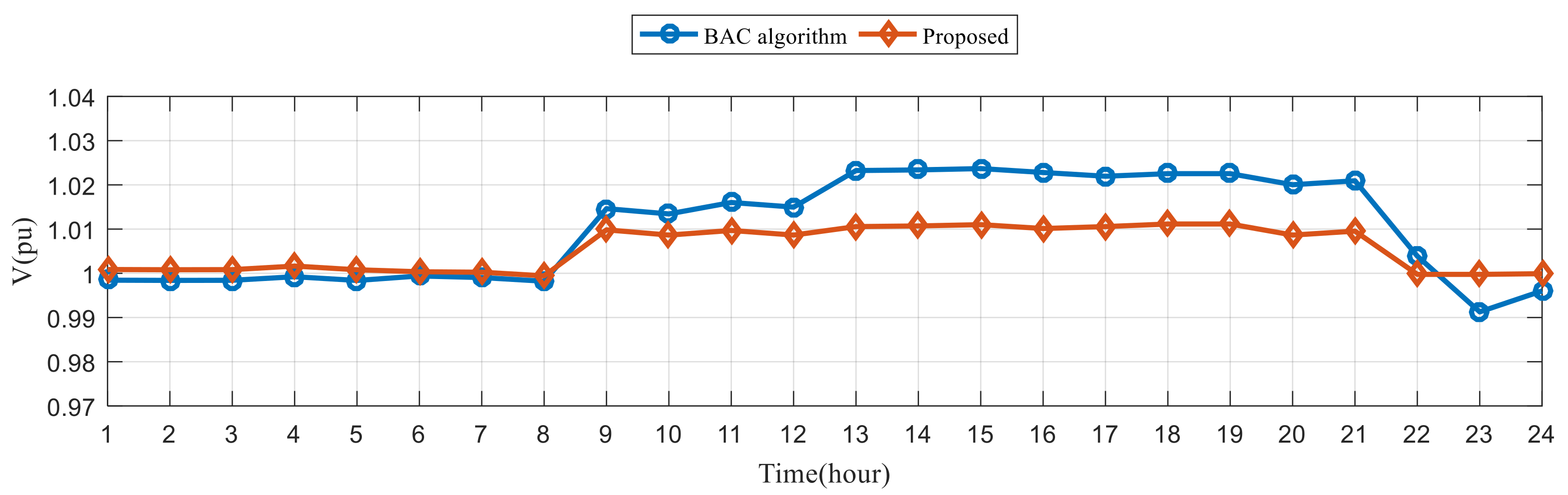
6.5. Simulation Results in IEEE 33 Bus System

Case 3 in the IEEE 33 bus system [34], shown in Figure 17, was adopted as a benchmark to verify the performance of the proposed method. In [34], an BAC algorithm was used. The objective functions and constraints are the same as those described in Section 2, and the validation indicators are the same as those in [34], where $J_1$ is the total system power loss, $J_2$ is the voltage deviation at the secondary side of the main transformer, $J_3$ is the voltage deviation at all buses, $J_4$ is the number of switching operations for the OLTC transformer, and $J_5$ is the number of switching operations for the SCs.

The voltages on the secondary side of the main transformer obtained using the two algorithms are shown in Figure 18. This shows that with the proposed method, the voltages are closer to the desired value (1.0 pu), and the voltage variation is evidently steadier.

Table 11. Results for different algorithms in the IEEE 33 bus system.

Method	${\mathit{J}}_1 \left(\mathbf{kWh}\right)$	${\mathit{J}}_2 \left(\mathbf{pu}\right)$	${\mathit{J}}_3 \left(\mathbf{pu}\right)$	${\mathit{J}}_4$	${\mathit{J}}_5$
BAC algorithm	864.43	0.2872	0.0039	9	7
Proposed method	887.93	0.1369	0.0027	4	7

presents the results for different algorithms in the IEEE 33 bus system. It can be observed that the voltage deviation, voltage variation, and switching costs are all smaller than those obtained in [34]. Regarding the power loss, the load demand is regarded as a constant power model: the higher the voltage, the smaller the power loss. Thus, power loss and voltage deviation are conflicting indicators. The results show that the power loss of the proposed method is higher, but not significantly different from that of the BAC algorithm. The proposed method performed better than the BAC algorithm in terms of voltage deviation.

7. Conclusions

In this study, a new method for distribution systems based on multi-objective voltage control was proposed. The main purpose was to determine the optimal daily schedule of switching operations for OLTC tap positions and SCs. For different DG power factors, DG locations, and DG capacities, the proposed method was compared with other voltage control methods. Compared with the LVL and RPDC methods, the percentage reductions in (1) voltage deviations at all buses, (2) voltage variations, (3) total system power loss, and (4) difference in values were as high as 160.93%, 31.16%, 10.35%, and 434.34%, respectively, using the proposed method. As can be seen, the proposed MOPSO performs better than previous voltage control methods in terms of various validation indicators and has better search ability. Compared with the PSO and GA algorithms, the proposed method delivered percentage reductions in the worst fitness of 3.66% and 0.96%, respectively, while the percentage reductions in standard deviation were 2514% and 488.11%, respectively. The proposed MOPSO is more effective than the other methods because it yields the best average fitness. On comparing the proposed method with other optimization algorithms on the IEEE 33 bus system, the proposed method was found to exhibit superior performance.

References

1. Renewable Capacity Statistics 2021; International Renewable Energy Agency (IRENA): Abu Dhabi, United Arab Emirates, 2021.
2. Yoshizawa, S.; Hayashi, Y. Predictive Voltage Control Scheme Based on Estimation of Short-Time-Ahead Voltage Fluctuation in Distribution System with Pvs. IEEJ Trans. Electr. Electron. Eng. 2021, 16, 916–924. [Google Scholar] [CrossRef]
3. Park, J.-Y.; Nam, S.-R.; Park, J.-K. Control of a ULTC considering the dispatch schedule of capacitors in a distribution system. IEEE Trans. Power Syst. 2007, 22, 755–761. [Google Scholar] [CrossRef]
4. Xiao, H.; Liu, G.; Huang, J.; Hou, S.; Zhu, L. Parameterized and centralized secondary voltage control for autonomous microgrids. Int. J. Electr. Power Energy Syst. 2022, 135, 107531. [Google Scholar] [CrossRef]
5. Šulc, P.; Backhaus, S.; Chertkov, M. Optimal distributed control of reactive power via the alternating direction method of multipliers. IEEE Trans. Energy Convers. 2014, 29, 968–977. [Google Scholar] [CrossRef]
6. Baker, K.; Bernstein, A.; Dall’anese, E.; Zhao, C.H. Network-Cognizant Voltage Droop Control for Distribution Grids. IEEE Trans. Power Syst. 2018, 33, 2098–2108. [Google Scholar] [CrossRef]
7. Di Fazio, A.R.; Fusco, G.; Russo, M. Decentralized Control of Distributed Generation for Voltage Profile Optimization in Smart Feeders. IEEE Trans. Smart Grid 2013, 4, 1586–1596. [Google Scholar] [CrossRef]
8. Elkhatib, M.E.; El Shatshat, R.; Salama, M.M. Decentralized reactive power control for advanced distribution automation systems. IEEE Trans. Smart Grid 2012, 3, 1482–1490. [Google Scholar] [CrossRef]
9. Qiao, F.; Ma, J. Voltage/Var Control for Hybrid Distribution Networks Using Decomposition-Based Multiobjective Evolutionary Algorithm. IEEE Access 2020, 8, 12015–12025. [Google Scholar] [CrossRef]
10. Elmitwally, A.; Elsaid, M.; Elgamal, M.; Chen, Z. A Fuzzy-Multiagent Self-Healing Scheme for a Distribution System with Distributed Generations. IEEE Trans. Power Syst. 2015, 30, 2612–2622. [Google Scholar] [CrossRef]
11. Bedawy, A.; Yorino, N.; Mahmoud, K.; Zoka, Y.; Sasaki, Y. Optimal Voltage Control Strategy for Voltage Regulators in Active Unbalanced Distribution Systems Using Multi-Agents. IEEE Trans. Power Syst. 2020, 35, 1023–1035. [Google Scholar] [CrossRef]
12. Kekatos, V.; Zhang, L.; Giannakis, G.B.; Baldick, R. Voltage regulation algorithms for multiphase power distribution grids. IEEE Trans. Power Syst. 2015, 31, 3913–3923. [Google Scholar] [CrossRef]
13. Wurl, T.; Lindner, M.; Witzmann, R. Analysis of interactions between regulated distribution transformers (RDT) and local voltage control Q(V) by means of the harmonic balance method. Int. J. Electr. Power Energy Syst. 2020, 120, 105901. [Google Scholar] [CrossRef]
14. Lindner, M.; Witzmann, R. Modelling and validation of an inverter featuring local voltage control Q(V) for transient stability and interaction analyses. Int. J. Electr. Power Energy Syst. 2018, 101, 280–288. [Google Scholar] [CrossRef]
15. Valverde, G.; Van Cutsem, T. Model predictive control of voltages in active distribution networks. IEEE Trans. Smart Grid 2013, 4, 2152–2161. [Google Scholar] [CrossRef]
16. Kim, Y.J.; Ahn, S.J.; Hwang, P.I.; Pyo, G.C.; Moon, S.I. Coordinated control of a DG and voltage control devices using a dynamic programming algorithm. IEEE Trans. Power Syst. 2013, 28, 42–51. [Google Scholar] [CrossRef]
17. Mahmoud, K.; Abdel-Nasser, M.; Lehtonen, M.; Hussein, M.M. Optimal Voltage Regulation Scheme for PV-Rich Distribution Systems Interconnected with D-STATCOM. Electr. Power Compon. Syst. 2021, 48, 2130–2143. [Google Scholar] [CrossRef]
18. Elkhatib, M.E.; El-Shatshat, R.; Salama, M.M.A. Novel coordinated voltage control for smart distribution networks with DG. IEEE Trans. Smart Grid 2011, 2, 598–605. [Google Scholar] [CrossRef]
19. Farag, H.E.Z.; El-Saadany, E.F. A Novel Cooperative Protocol for Distributed Voltage Control in Active Distribution Systems. IEEE Trans. Power Syst. 2013, 28, 1645–1656. [Google Scholar] [CrossRef]
20. Agalgaonkar, Y.P.; Pal, B.C.; Jabr, R.A. Distribution voltage control considering the impact of PV generation on tap changers and autonomous regulators. IEEE Trans. Power Syst. 2013, 29, 182–192. [Google Scholar] [CrossRef]
21. Mufaris, A.L.M.; Baba, J.; Yoshizawa, S.; Hayashi, Y. Determination of dynamic line drop compensation parameters of voltage regulators for voltage rise mitigation. In Proceedings of the 2015 International Conference on Clean Electrical Power (ICCEP), Taormina, Italy, 16–18 June 2015; pp. 319–325. [Google Scholar]
22. Kim, M.; Hara, R.; Kita, H. Design of the optimal ULTC parameters in distribution system with distributed generations. IEEE Trans. Power Syst. 2009, 24, 297–305. [Google Scholar]
23. Chen, Y.; Strothers, M.; Benigni, A. All-day coordinated optimal scheduling in distribution grids with PV penetration. Electr. Power Syst. Res. 2018, 164, 112–122. [Google Scholar] [CrossRef]
24. Zhang, L.; Tang, W.; Liang, J.; Cong, P.; Cai, Y. Coordinated day-ahead reactive power dispatch in distribution network based on real power forecast errors. IEEE Trans. Power Syst. 2015, 31, 2472–2480. [Google Scholar] [CrossRef]
25. Ferraz, B.P.; Resener, M.; Pereira, L.A.; Lemos, F.A.; Haffner, S. MILP model for volt-var optimization considering chronological operation of distribution systems containing DERs. Int. J. Electr. Power Energy Syst. 2021, 129, 106761. [Google Scholar] [CrossRef]
26. Ozdemir, G.; Baran, M. A new method for Volt–Var optimization with conservation voltage reduction on distribution systems. Electr. Eng. 2020, 102, 493–502. [Google Scholar] [CrossRef]
27. Kim, Y.J.; Kirtley, J.L.; Norford, L.K. Reactive Power Ancillary Service of Synchronous Dgs in Coordination with Voltage Control Devices. IEEE Trans. Smart Grid 2017, 8, 515–527. [Google Scholar] [CrossRef]
28. Heydarianasl, M.; Rahmat, M.F. Design optimization of electrostatic sensor electrodes via MOPSO. Measurement 2020, 152, 107288. [Google Scholar] [CrossRef]
29. Sivaranjani, R.; Roomi, S.M.M.; Senthilarasi, M. Speckle noise removal in SAR images using Multi-Objective PSO (MOPSO) algorithm. Appl. Soft Comput. 2019, 76, 671–681. [Google Scholar] [CrossRef]
30. Ghorbani, N.; Kasaeian, A.; Toopshekan, A.; Bahrami, L.; Maghami, A. Optimizing a hybrid wind-PV-battery system using GA-PSO and MOPSO for reducing cost and increasing reliability. Energy 2018, 154, 581–591. [Google Scholar] [CrossRef]
31. Qiu, G.X.; Zhan, D.P.; Jiang, Z.H.; Zhang, H.S. Optimisation of the MgO/Al2O3 ratio of high-alumina BF slag based on MOPSO algorithm. Ironmak. Steelmak. 2019, 46, 712–720. [Google Scholar] [CrossRef]
32. Reyes-Sierra, M.; Coello, C.C. Multi-objective particle swarm optimizers: A survey of the state-of-the-art. Int. J. Comput. Intell. Res. 2006, 2, 287–308. [Google Scholar]
33. Chiu, W.-Y.; Yen, G.G.; Juan, T.-K. Minimum Manhattan distance approach to multiple criteria decision making in multiobjective optimization problems. IEEE Trans. Evol. Comput. 2016, 20, 972–985. [Google Scholar] [CrossRef]
34. Azimi, R.; Esmaeili, S. Multiobjective daily Volt/VAr control in distribution systems with distributed generation using binary ant colony optimization. Turk. J. Electr. Eng. Comput. Sci. 2013, 21, 613–629. [Google Scholar] [CrossRef]
Figure 1. Data exchange between DIgSILENT and MATLAB.
Mathematics 10 02969 g001
Figure 2. Pareto front for a two-objective problem.
Mathematics 10 02969 g002
Figure 3. Two solutions for a two-objective problem.
Mathematics 10 02969 g003
Figure 7. Sample system.
Mathematics 10 02969 g007
Figure 8. Daily load curve on the secondary side of the main transformer.
Mathematics 10 02969 g008
Figure 9. Voltage variations at different buses and OLTC tap position and SCs operation schedule over a day when DG is connected to bus A3 with 0.95 power factor lagging—Case 01.
Mathematics 10 02969 g009
Figure 10. Voltages at bus A2 for different methods—Case 01.
Mathematics 10 02969 g010
Figure 11. Voltages at bus A2 for different methods—Case 02.
Mathematics 10 02969 g011
Figure 12. Voltages at bus A2 for different methods—Case 03.
Mathematics 10 02969 g012
Figure 13. Voltages at bus A2 for different methods—Case 04.
Mathematics 10 02969 g013
Figure 14. Voltages at bus A2 for different methods—Case 05.
Mathematics 10 02969 g014
Figure 15. Voltages at bus A2 for different methods—Case 06.
Mathematics 10 02969 g015
Figure 16. Hourly voltage deviations at bus A2 for three different voltage control methods.
Mathematics 10 02969 g016
Figure 17. IEEE 33 bus test system.
Mathematics 10 02969 g017
Figure 18. Voltages at the secondary side of the main transformer.
Mathematics 10 02969 g018