Two Regularization Methods for the Variational Inequality Problem over the Set of Solutions of the Generalized Mixed Equilibrium Problem

Abstract

In this work, we consider bilevel problems: variational inequality problems over the set of solutions of the generalized mixed equilibrium problems. Two new inertial extragradient methods are proposed for solving these problems. Under appropriate conditions, we prove strong convergence theorems for the proposed methods by the regularization technique. Finally, some numerical examples are provided to show the efficiency of the proposed algorithms.

1. Introduction

Let $\mathcal{H}$ be a Hilbert space with the inner product $\langle ·,·\rangle$ and the induced norm $∥·∥$. Let $\mathcal{C}$ be a closed, convex and nonempty subset of a real Hilbert space $\mathcal{H}$. Let $\mathrm{\Psi }:\mathcal{C}\times \mathcal{C}\to \mathbb{R}$ be a nonlinear bifunction, $\mathcal{A}:\mathcal{C}\to \mathcal{H}$ be a nonlinear mapping, and $\mathrm{\Phi }:C\to \mathbb{R}\bigcup \{+\infty \}$ be a proper convex lower semicontinuous function. The generalized mixed equilibrium problem (GMEP) is defined as:

$$\mathrm{Find}\mathrm{a}\mathrm{point}{u}^{*}\in \mathcal{C}\mathrm{such}\mathrm{that}\mathrm{\Psi }(u^{*},v)+\mathrm{\Phi }\left(v\right)-\mathrm{\Phi }\left(u^{*}\right)+\langle \mathcal{A}{u}^{*},v-u^{*}\rangle \ge 0,\forall v\in \mathcal{C}.$$

(1)

The set of solutions of (1) is denoted by $\mathrm{GMEP}(\mathrm{\Psi },\mathrm{\Phi },\mathcal{A})$. Next, we provide some special cases of the GMEP (1).

(I) If $\mathcal{A}=0$, the GMEP (1) reduces to the mixed equilibrium problem (MEP):

$$\mathrm{Find}\mathrm{a}\mathrm{point}{u}^{*}\in \mathcal{C}\mathrm{such}\mathrm{that}\mathrm{\Psi }(u^{*},v)+\mathrm{\Phi }\left(v\right)-\mathrm{\Phi }\left(u^{*}\right)\ge 0,\forall v\in \mathcal{C}.$$

(2)

The set of solutions of the MEP (2) is denoted by $\mathrm{MEP}(\mathrm{\Psi },\mathrm{\Phi })$.

(II) If $\mathrm{\Phi }=0$, the GMEP (1) becomes the generalized equilibrium problem (GEP):

$$\mathrm{Find}\mathrm{a}\mathrm{point}{u}^{*}\in \mathcal{C}\mathrm{such}\mathrm{that}\mathrm{\Psi }(u^{*},v)+\langle \mathcal{A}{u}^{*},v-u^{*}\rangle \ge 0,\forall v\in \mathcal{C}.$$

(3)

The set of solutions of the GEP (3) is denoted by $\mathrm{GEP}(\mathrm{\Psi },\mathcal{A})$. Particularly, if $\mathcal{A}=0$ in (3), the GEP reduces to the classical equilibrium problem which is to

$$\mathrm{find}\mathrm{a}\mathrm{point}{u}^{*}\in \mathcal{C}\mathrm{such}\mathrm{that}\mathrm{\Psi }(u^{*},v)\ge 0,\forall v\in \mathcal{C}.$$

(4)

The GMEP is a generalization of many mathematical models such as saddle point problems, variational inequality problems, fixed point problems, minimization problems, certain optimization problems, Nash equilibrium problems, and others, see [1,2,3,4,5] for examples. Many authors have studied and proposed several iterative algorithms for solving GMEPs and related optimization problems; see for instance [6,7,8].

(III) If $\mathrm{\Psi }(u,v)=0$ for all $u,v\in \mathcal{C}$ and $\mathrm{\Phi }\left(u\right)=0$ for all $u\in \mathcal{C},$ then the GMEP (1) reduces to the variational inequality problem (VIP):

$$\mathrm{Find}\mathrm{a}\mathrm{point}{u}^{*}\in \mathcal{C}\mathrm{such}\mathrm{that}\langle \mathcal{A}{u}^{*},v-u^{*}\rangle \ge 0,\forall v\in \mathcal{C},$$

(5)

which solution set is denoted by $\mathrm{VI}(\mathcal{C},\mathcal{A})$. The VIP was first introduced by Fichera [9] in 1963 as Signori’s contact problem. Later, it was studied by Stampacchia [10] for modeling problems arising from mechanics. This problem is also known to have numerous applications in diverse fields such as, engineering, physics, mathematical programming, economics, among others. It can be considered as a central problem in nonlinear analysis and optimization since the theory of variational inequalities provides a natural, convenient, and unified framework for many network equilibrium problems, minimization problems, systems of nonlinear equations, complementary problems, and others (see [11,12,13]). Hence, the theory has become an area of great interest to numerous researchers. As a result of this, there has been an increased interest in developing implementable and efficient methods for solving VIPs.

Many methods for solving the variational inequality (1) have been introduced and studied (see, for example, [14,15,16]). One of the popular methods is the extragradient method (EGM), which was proposed by Korpelevich [7] (and also independently Antipin [17]) for solving the saddle point problems. It was subsequently extended to the VIPs with monotone and Lipschitz continuous mappings in both Euclidean spaces and Hilbert spaces. More precisely, the EGM is described as follows:

$$\left\{\begin{array}{c}{y}_n=P_{\mathcal{C}}(x_n-r\mathcal{A}{x}_n),\hfill \\ x_{n+1}=P_{\mathcal{C}}(x_n-r\mathcal{A}{y}_n),\hfill \end{array}\right.$$

(6)

where $r\in (0,1/L)$. Note that the EGM might require a prohibitive amount of computation time when the structure of the feasible set $\mathcal{C}$ is complex. This can affect the efficiency of the used method. In an attempt to overcome this computational drawback, Tseng [18] introduced a new extragradient method (TEGM) which is stated as follows.

One of the novelties in the proposed TEGM is that it requires only one projection per iteration. It is worth pointing out that the TEGM needs to know the information or approximation of the Lipschitz constant of $\mathcal{A}$, which limits the applicability of the method. On the other hand, we note that under some appropriate settings, Equation (6) and Algorithm 1 converge to the solution of the variational inequality weakly. However, Bauschke and Combettes [19] remarked that strong convergence is more desirable than weak convergence in solving some optimization problems. In order to establish a strongly convergent Algorithm 2 which does not require prior knowledge of the Lipschitz constants of $\mathcal{A}$, Yang et al. [20] suggested a new self-adaptive Tseng’s extragradient method (STEM):

Algorithm 1 Tseng’s extragradient method (TEGM).

Initialization: Take $r>0$ and let $x_1\in \mathcal{H}$ be arbitrary. Step 1. Given $x_n(n\ge 1)$, compute $$y_n=P_{\mathcal{C}}(x_n-r\mathcal{A}{x}_n).$$ Step 2. Calculate the next iterate $$x_{n+1}=y_n-r(\mathcal{A}{y}_n-\mathcal{A}{x}_n).$$

Algorithm 2 Self-adaptive Tseng’s extragradient method (STEM).

Initialization: Take $\left\{{\alpha }_n\right\}\subset (0,+\infty )$, $r_1>0$, $\upsilon \in (0,1)$ and let $x_1\in \mathcal{H}$ be arbitrary. Step 1. Given $x_n(n\ge 1)$, compute $$y_n=P_{\mathcal{C}}\left(x_n-r_n\mathcal{A}{x}_n\right),$$ and $$z_n=y_n-r_n(\mathcal{A}{y}_n-\mathcal{A}{x}_n),$$ where $\left\{r_n\right\}$ is updated by $$r_{n+1}=\left\{\begin{array}{c}min\{\frac{\upsilon ∥x_n-y_n∥}{∥\mathcal{A}{x}_n-\mathcal{A}{y}_n∥},r_n\},\mathrm{if}\mathcal{A}{x}_n-\mathcal{A}{y}_n\ne 0;\hfill \\ r_n,\mathrm{otherwise}.\hfill \end{array}\right.$$ If $x_n=y_n$, then stop: $x_n$ is a solution. Otherwise, go to Step 2. Step 2. Compute $$x_{n+1}={\alpha }_{n}g\left(x_n\right)+(1-{\alpha }_n)z_n.$$ Step 3. Set $n:=n+1$ and go to Step 1.

Under mild conditions, they proved the strong convergence of the introduced method to an element of $\mathrm{VI}(\mathcal{C},\mathcal{A})$. The algorithm proposed in [20] applies a new step size criterion that automatically updates the iteration stepsize by a simple computation using some previously known information. However, this method generates a monotonically decreasing sequence of stepsize and might further affect the execution efficiency of such method.

Motivated by the ideas of the EGM, the TEGM, and the STEM, Tan and Qin [8] proposed a new inertial extragradient method with non-monotonic stepsizes (SVTE) for solving the VIPs as follows:

They proved strong convergence of Algorithm 3 to an element of $\mathrm{VI}(\mathcal{C},\mathcal{A})$ under appropriate conditions.

Algorithm 3 Self adaptive viscosity-type inertial Tseng’s extragradient algorithm (SVTE).

Initialization: Take $\left\{{ϵ}_n\right\}\subset (0,+\infty )$, $\left\{{\sigma }_n\right\}\subset (0,+\infty )$, $\left\{{\alpha }_n\right\}\subset (0,+\infty )$, $\varrho >0$, $r_1>0$, $\upsilon \in (0,1)$ and let $x_0,x_1\in \mathcal{H}$ be arbitrary. Step 1. Given $x_{n-1}$ and $x_n(n\ge 1)$, compute $$u_n=x_n+h_n(x_n-x_{n-1}),$$ where $${\tau }_n=\left\{\begin{array}{c}min\{\frac{{ϵ}_n}{∥x_n-x_{n-1}∥},\varrho \},\mathrm{if}{x}_n\ne x_{n-1};\hfill \\ \varrho ,\mathrm{otherwise}.\hfill \end{array}\right.$$ (7) Step 2. Compute $$y_n=P_{\mathcal{C}}\left(u_n-r_n\mathcal{A}{u}_n\right),$$ and $$z_n=y_n-r_n(\mathcal{A}{y}_n-\mathcal{A}{x}_n),$$ where $\left\{r_n\right\}$ is updated by $$r_{n+1}=\left\{\begin{array}{c}min\{\frac{\upsilon ∥u_n-y_n∥}{∥\mathcal{A}{u}_n-\mathcal{A}{y}_n∥},r_n+{\sigma }_n\},\mathrm{if}\mathcal{A}{u}_n-\mathcal{A}{y}_n\ne 0;\hfill \\ r_n+{\sigma }_n,\mathrm{otherwise}.\hfill \end{array}\right.$$ (8) Step 3. Compute $$x_{n+1}={\alpha }_{n}g\left(x_n\right)+(1-{\alpha }_n)z_n.$$ Step 5. Set $n:=n+1$ and back to Step 1.

Recently, a great deal of effort has been devoted to the bilevel variational inequality problem (BVIP) which consists of the following:

$$\mathrm{Find}{u}^{*}\in \mathrm{VI}(\mathcal{C},\mathcal{A}),\mathrm{such}\mathrm{that},\langle \mathcal{F}{u}^{*},v-u^{*}\rangle \ge 0,\forall v\in \mathrm{VI}(\mathcal{C},\mathcal{A}),$$

(9)

where $\mathcal{A}:\mathcal{C}\to \mathcal{H}$ and $\mathcal{F}:\mathcal{C}\to \mathcal{H}$ are two single-valued mappings. Mathematically, as observed, the problem BVIP is very general in the sense that it includes, as special cases, the complementarity problem, variational inequality problem, Nash equilibrium problem, fixed point problem, as well as the optimization problem; see, e.g., [21,22,23].

Since the VIP is a special case of the GMEP (see, e.g., [24]) then, it is necessary to improve the BVIP to more general bilevel problems and propose effective methods for approximating numerical solutions to these bilevel problems.

The purpose of this paper is to analyze and study a more general bilevel problem: a variational inequality over the set of solutions of the generalized mixed equilibrium problem (VOGME). More precisely, the VOGME is presented as follows:

$$\mathrm{Find}{u}^{*}\in \mathrm{GMEP}(\mathrm{\Psi },\mathrm{\Phi },\mathcal{A}),\mathrm{such}\mathrm{that},\langle \mathcal{F}{u}^{*},v-u^{*}\rangle \ge 0,\forall v\in \mathrm{GMEP}(\mathrm{\Psi },\mathrm{\Phi },\mathcal{A}),$$

(10)

where $\mathrm{\Psi }$ is a bifunction, $\mathcal{F}$ is strongly monotone, and $\mathcal{A}$ is monotone. Combining the TEGM, the inertial idea and regularization technique, we propose two alternative methods for solving the VOGME (10). The strong convergence theorems of the suggested algorithms is established under appropriate and weaker conditions. The theoretical results are also confirmed by two numerical examples.

2. Preliminaries

Throughout this section, let $\mathcal{C}$ be a nonempty closed convex subset of a Hilbert space $\mathcal{H}$. We now recall the following concepts of mappings and lemmas for the convergence analysis of our methods.

Notation 1.

Let $\left\{x_n\right\}$ be a sequence and x be a point in a Hilbert space $\mathcal{H}$.

• $x_n\to x$ means that $\left\{x_n\right\}$ converges to x strongly;
• $x_n\rightharpoonup x$ means that $\left\{x_n\right\}$ converges to x weakly;
• $\omega \left(x_n\right)$ denotes the set of weak limits of $\left\{x_n\right\}$, i.e., $\omega \left(x_n\right):=\{x:x_{n_j}\rightharpoonup x\}$;
• $\mathrm{Fix}\left(\mathcal{T}\right)$ denotes the set of fixed points of a mapping $\mathcal{T}$.

Definition 1.

A mapping $\mathcal{T}:\mathcal{C}\to \mathcal{H}$ is said to be:

(i) 

monotone, if

$$\langle \mathcal{T}x-\mathcal{T}y,x-y\rangle \ge 0,\forall x,y\in \mathcal{C};$$

(ii) 

α- strongly monotone, if there exists a number $\alpha >0$ such that

$$\langle \mathcal{T}x-\mathcal{T}y,x-y\rangle \ge \alpha {∥x-y∥}^2,\forall x,y\in \mathcal{C};$$

(iii) 

λ-inverse strongly monotone, if there exists a positive number λ such that

$$\langle \mathcal{T}x-\mathcal{T}y,x-y\rangle \ge \lambda {∥\mathcal{T}x-\mathcal{T}y∥}^2,\forall x,y\in C;$$

(iv) 

k- Lipschitz continuous, if there exists $k>0$ such that

$$∥\mathcal{T}x-\mathcal{T}y∥\le k∥x-y∥,\forall x,y\in \mathcal{C}.$$

Definition 2.

The equilibrium bifunction $\mathrm{\Psi }:\mathcal{C}\times \mathcal{C}\to \mathbb{R}$ is said to be monotone, if

$$\mathrm{\Psi }(x,y)+\mathrm{\Psi }(y,x)\le 0,\forall x,y\in \mathcal{C}.$$

Definition 3.

A single-valued operator $\mathcal{A}:\mathcal{C}\to \mathcal{H}$ is said to be hemicontinuous if the real function

$$t\mapsto \langle A\left(\right(1-t)u+tv),w\rangle$$

is continuous on $[0,1]$ for all $u,v,w\in \mathcal{C}$.

Lemma 1

([14]). Let $\left\{z_n\right\}$ be a sequence of nonnegative real numbers. Assume that

$$z_{n+1}\le (1-a_n)z_n+b_n,n\in \mathbb{N},$$

where $\left\{a_n\right\},\left\{b_n\right\}$ satisfy the conditions

(i) 

${\sum }_{n=1}^{\infty }{a}_n=\infty ,{lim}_{n\to \infty }{a}_n=0$,

(ii) 

${lim\; sup}_{n\to \infty }\frac{b_n}{a_n}\le 0$.

Then, ${lim}_{n\to \infty }{z}_n=0$.

Assumption 1.

Let $\mathcal{C}$ be a nonempty, convex, and closed subset of a Hilbert space $\mathcal{H}$, and Ψ: $\mathcal{C}\times \mathcal{C}\to \mathbb{R}$ be a bifunction satisfying the following restrictions:

(A1) 

$\mathrm{\Psi }(x,x)=0$, $\forall x\in \mathcal{C}$;

(A2) 

Ψ is monotone;

(A3) 

${lim\; sup}_{t\to 0^{+}}\mathrm{\Psi }(x+t(z-x),y)\le \mathrm{\Psi }(x,y),\forall x,y,z\in \mathcal{C}$;

(A4) 

for all $x\in \mathcal{C},\mathrm{\Psi }(x,·)$ is convex and lower semicontinuous.

Lemma 2

([1]). Let $\mathrm{\Psi }:\mathcal{C}\times \mathcal{C}\to \mathbb{R}$ be a bifunction satisfying Assumption 1 (A1)–(A4). For $x\in \mathcal{H}$ and $r>0$, define a mapping $J_r:\mathcal{H}\to \mathcal{C}$ by:

$$J_{r}x=\{z\in \mathcal{C}:\mathrm{\Psi }(z,y)+\frac{1}{r}\langle y-z,z-x\rangle \ge 0,\forall y\in \mathcal{C}\}.$$

Then, the following results hold:

(i) 

$J_{r}x\ne \varnothing$ for each $x\in \mathcal{H}$;

(ii) 

$J_r$ is single-valued;

(iii) 

$J_r$ is a firmly nonexpansive mapping, i.e., for all $x,y\in \mathcal{H},$${∥J_{r}x-J_{r}y∥}^2\le \langle J_{r}x-J_{r}y,x-y\rangle ;$

(iv) 

$\mathrm{Fix}\left(J_r\right)=\mathrm{EP}\left(\mathrm{\Psi }\right);$

(v) 

$\mathrm{EP}\left(\mathrm{\Psi }\right)$ is closed and convex.

Lemma 3.

Let $\mathcal{A}:\mathcal{C}\to \mathcal{H}$ be monotone and hemicontinuous, $\mathrm{\Phi }:\mathcal{C}\to \mathbb{R}$ be a proper lower semicontinuous and convex function, and $\mathrm{\Psi }:\mathcal{C}\times \mathcal{C}\to \mathbb{R}$ be a bifunction satisfying Assumption 1 (A1)–(A4). Then the $\mathrm{GMEP}$ (1) is equivalent to the following problem:

$$Find\mathrm{a}point{u}^{*}\in \mathcal{C}suchthat-\mathrm{\Psi }(v,u^{*})+\mathrm{\Phi }\left(v\right)-\mathrm{\Phi }\left(u^{*}\right)+\langle \mathcal{A}v,v-u^{*}\rangle \ge 0,\forall v\in \mathcal{C}.$$

(11)

Proof. 

Let $u^{*}\in \mathcal{C}$ be a solution of the GMEP (1). We find from Assumption 1 (A2) and the monotonicity of $\mathcal{A}$ that

$$\begin{array}{ccc}\hfill & & -\mathrm{\Psi }(v,u^{*})+\mathrm{\Phi }\left(v\right)-\mathrm{\Phi }\left(u^{*}\right)+\langle \mathcal{A}v,v-u^{*}\rangle \hfill \\ & \ge & \mathrm{\Psi }(u^{*},v)+\mathrm{\Phi }\left(v\right)-\mathrm{\Phi }\left(u^{*}\right)+\langle \mathcal{A}{u}^{*},v-u^{*}\rangle \hfill \\ & \ge & 0.\hfill \end{array}$$

(12)

Thus, $u^{*}\in \mathcal{C}$ is a solution of the problem (11).

Conversely, let $u^{*}\in \mathcal{C}$ be a solution of the problem (11). Setting $v_t=(1-t)u^{*}+tv$ for all $v\in \mathcal{C}$, then $v_t\in \mathcal{C}$. Since $u^{*}\in \mathcal{C}$ is a solution of the problem (11), it follows that

$$-\mathrm{\Psi }(v_t,u^{*})+\mathrm{\Phi }\left(v_t\right)-\mathrm{\Phi }\left(u^{*}\right)+\langle \mathcal{A}{v}_t,v_t-u^{*}\rangle \ge 0.$$

(13)

Utilizing Assumption 1 (A1) and (A4), we deduce

$$\begin{array}{ccc}\hfill 0& =& \mathrm{\Psi }(v_t,v_t)\hfill \\ & \le & (1-t)\mathrm{\Psi }(v_t,u^{*})+t\mathrm{\Psi }(v_t,v)\hfill \\ & =& (1-t)[\mathrm{\Psi }(v_t,u^{*})-\mathrm{\Phi }\left(v_t\right)+\mathrm{\Phi }\left(u^{*}\right)-\langle \mathcal{A}{v}_t,v_t-u^{*}\rangle ]+t\mathrm{\Psi }(v_t,v)\hfill \\ & & +(1-t)[\mathrm{\Phi }\left(v_t\right)-\mathrm{\Phi }\left(u^{*}\right)+\langle \mathcal{A}{v}_t,v_t-u^{*}\rangle ].\hfill \end{array}$$

(14)

Substituting (13) into (14), we obtain

$$0\le t\mathrm{\Psi }(v_t,v)+(1-t)[\mathrm{\Phi }\left(v_t\right)-\mathrm{\Phi }\left(u^{*}\right)+\langle \mathcal{A}{v}_t,v_t-u^{*}\rangle ].$$

(15)

Due to the assumption that $\mathrm{\Phi }$ is convex, we derive that

$$\begin{array}{c}\hfill \mathrm{\Phi }\left(v_t\right)-\mathrm{\Phi }\left(u^{*}\right)+\langle \mathcal{A}{v}_t,v_t-u^{*}\rangle \le t[\mathrm{\Phi }\left(v\right)-\mathrm{\Phi }\left(u^{*}\right)+\langle \mathcal{A}{v}_t,v-u^{*}\rangle ].\end{array}$$

(16)

Substituting (16) into (15), we find

$$\begin{array}{ccc}\hfill 0& \le & t\mathrm{\Psi }(v_t,v)+(1-t)t[\mathrm{\Phi }\left(v\right)-\mathrm{\Phi }\left(u^{*}\right)+\langle \mathcal{A}{v}_t,v-u^{*}\rangle ],\hfill \end{array}$$

which yields

$$\begin{array}{ccc}\hfill 0& \le & \mathrm{\Psi }(v_t,v)+(1-t)[\mathrm{\Phi }\left(v\right)-\mathrm{\Phi }\left(u^{*}\right)+\langle \mathcal{A}{v}_t,v-u^{*}\rangle ].\hfill \end{array}$$

By allowing $t\to 0$, noting (A3) and hemicontinuous continuity of $\mathcal{A}$, we derive

$$\begin{array}{ccc}\hfill 0& \le & \mathrm{\Psi }(u^{*},v)+\mathrm{\Phi }\left(v\right)-\mathrm{\Phi }\left(u^{*}\right)+\langle \mathcal{A}{u}^{*},v-u^{*}\rangle .\hfill \end{array}$$

Hence, we conclude that $u^{*}\in \mathcal{C}$ is a solution of the GMEP (1). This completes the proof.    □

Applying Lemma 3, we can obtain the following results immediately.

Corollary 1

([25]). Suppose $\mathcal{A}:\mathcal{C}\to \mathcal{H}$ is a hemicontinuous and monotone operator, then $u^{*}$ is a solution of the $\mathrm{VIP}$ (5) if and only if $u^{*}$ is a solution of the following problem:

$$Find{u}^{*}\in \mathcal{C}suchthat\langle \mathcal{A}v,v-u^{*}\rangle \ge 0,\forall v\in \mathcal{C}.$$

Lemma 4.

Let $\mathcal{A}:\mathcal{C}\to \mathcal{H}$ be monotone and hemicontinuous, $\mathrm{\Phi }:\mathcal{C}\to \mathbb{R}$ be a proper lower semicontinuous and convex function, and $\mathrm{\Psi }:\mathcal{C}\times \mathcal{C}\to \mathbb{R}$ be a bifunction satisfying Assumption 1 (A1)–(A4). For $x\in \mathcal{H}$ and $r>0$, define a mapping $T_r:\mathcal{H}\to \mathcal{C}$ by:

$$T_{r}x=\{z\in \mathcal{C}:\mathrm{\Psi }(z,y)+\langle \mathcal{A}z,y-z\rangle +\mathrm{\Phi }\left(y\right)-\mathrm{\Phi }\left(z\right)+\frac{1}{r}\langle y-z,z-x\rangle \ge 0,\forall y\in \mathcal{C}\}.$$

Then, the following results hold:

(i) 

$T_{r}x\ne \varnothing$ for each $x\in \mathcal{H}$;

(ii) 

$T_r$ is single-valued;

(iii) 

$T_r$ is a firmly nonexpansive mapping;

(iv) 

$\mathrm{Fix}\left(T_r\right)=\mathrm{GMEP}(\mathrm{\Psi },\mathrm{\Phi },\mathcal{A});$

(v) 

$\mathrm{GMEP}(\mathrm{\Psi },\mathrm{\Phi },\mathcal{A})$ is closed and convex.

Furthermore, if $\mathcal{A}$ is β-strongly monotone, then it also holds that

(iii)’ 

$T_r$ is a contraction on C with contraction coefficient $\frac{1}{1+r\beta }.$

Proof. 

Letting $\tilde{F}(x,y)=\mathrm{\Psi }(x,y)+\mathrm{\Phi }\left(y\right)-\mathrm{\Phi }\left(x\right)+\langle \mathcal{A}x,y-x\rangle ,\forall x,y\in \mathcal{C},$ it is not difficult to check that $\tilde{F}$ satisfies Assumption 1 (A1)–(A4). Then one finds from Lemma 2 that (i)–(v) holds. Further, if $\mathcal{A}$ is $\beta$-strongly monotone, then we have, for $\forall x,y\in \mathcal{H}$:  

$$\begin{array}{ccc}& & \mathrm{\Psi }(T_{r}x,T_{r}y)+\langle \mathcal{A}{T}_{r}x,T_{r}y-T_{r}x\rangle +\mathrm{\Phi }\left(T_{r}y\right)-\mathrm{\Phi }\left(T_{r}x\right)\hfill \\ & & +\frac{1}{r}\langle T_{r}y-T_{r}x,T_{r}x-x\rangle \ge 0,\hfill \end{array}$$

and

$$\begin{array}{ccc}& & \mathrm{\Psi }(T_{r}y,T_{r}x)+\langle \mathcal{A}{T}_{r}y,T_{r}x-T_{r}y\rangle +\mathrm{\Phi }\left(T_{r}x\right)-\mathrm{\Phi }\left(T_{r}y\right)\hfill \\ & & +\frac{1}{r}\langle T_{r}x-T_{r}y,T_{r}y-y\rangle \ge 0.\hfill \end{array}$$

Adding the two inequalities, noticing Assumption 1 (A2) and the $\beta$-strong monotonicity of $\mathcal{A}$, we have

$$\begin{array}{c}\hfill -\beta {∥T_{r}y-T_{r}x∥}^2-\frac{1}{r}{∥T_{r}y-T_{r}x∥}^2+\frac{1}{r}\langle T_{r}y-T_{r}x,y-x\rangle \ge 0,\end{array}$$

which is equivalent to

$$\begin{array}{c}\hfill (1+r\beta ){∥T_{r}y-T_{r}x∥}^2\le \langle T_{r}y-T_{r}x,y-x\rangle .\end{array}$$

Thus,

$$\begin{array}{c}\hfill ∥T_{r}y-T_{r}x∥\le \frac{1}{1+r\beta }∥y-x∥.\end{array}$$

This implies $T_r$ is contractive with contraction coefficient $\frac{1}{1+r\beta }.$ This is the desired result ${\left(iii\right)}^{\prime }$.    □

If $\mathcal{A}=0$ for all $x\in \mathcal{C}$ in Lemma 4, then we obtain the following corollary.

Corollary 2.

Let $\mathrm{\Phi }:\mathcal{C}\to \mathbb{R}$ be a proper lower semicontinuous and convex function, and $\mathrm{\Psi }:\mathcal{C}\times \mathcal{C}\to \mathbb{R}$ be a bifunction satisfying Assumption 1 (A1)–(A4). Let the mapping $K_r:\mathcal{H}\to \mathcal{C}$ defined by

$$K_r\left(x\right)=\{z\in \mathcal{C}:\mathrm{\Psi }(z,y)+\mathrm{\Phi }\left(y\right)-\mathrm{\Phi }\left(z\right)+\frac{1}{r}\langle y-z,z-x\rangle \ge 0,\forall y\in \mathcal{C}\}.$$

Then, we find that

(i) 

$K_r\left(x\right)\ne \varnothing$ for each $x\in \mathcal{H}$;

(ii) 

$K_r$ is single-valued;

(iii) 

$K_r$ is a firmly nonexpansive mapping;

(iv) 

$\mathrm{Fix}\left(K_r\right)=\mathrm{MEP}(\mathrm{\Psi },\mathrm{\Phi });$

(v) 

$\mathrm{MEP}(\mathrm{\Psi },\mathrm{\Phi })$ is closed and convex.

3. Main Results

In this section, we aim to establish strong convergence results for the VOGME (10) by using Tseng’s extragradient method, the inertial idea, and the regularization method. In what follows, let $\mathcal{C}$ be a nonempty closed convex subset of a Hilbert space $\mathcal{H}$. Suppose that $\mathrm{\Psi }:\mathcal{C}\times \mathcal{C}\to \mathbb{R}$ is a bifunction satisfying Assumption 1 (A1)–(A4), $\mathrm{\Phi }:\mathcal{C}\to \mathbb{R}$ is a proper lower semicontinuous and convex function $\mathcal{A}:\mathcal{H}\to \mathcal{H}$ is monotone, and L-Lipschitz continuous, $\mathcal{F}:\mathcal{H}\to \mathcal{H}$ is h-strongly monotone and k-Lipschitz continuous. Additionally, we also assume that $\mathrm{GMEP}(\mathrm{\Psi },\mathrm{\Phi },\mathcal{A})$ is nonempty. One finds from Lemma 4 (v) that $\mathrm{GMEP}(\mathrm{\Psi },\mathrm{\Phi },\mathcal{A})$ is closed and convex. This, by strong monotonicity and continuity of $\mathcal{F}$, ensures the uniqueness of solutions $x^{†}$ to the VOGME (10). Together with the GMEP (1), we consider the following regularized generalized mixed equilibrium problem (RGMEP) for each $\alpha >0$: Find a point $x\in \mathcal{C}$ such that

$$\mathrm{\Psi }(x,y)+\mathrm{\Phi }\left(y\right)-\mathrm{\Phi }\left(x\right)+\langle \mathcal{A}x+\alpha \mathcal{F}x,y-x\rangle \ge 0,\forall y\in \mathcal{C}.$$

(17)

Under the above assumptions, one deduces that the mapping $\tilde{\mathcal{A}}:=\mathcal{A}+\alpha \mathcal{F}$ is strongly monotone for all $\alpha >0.$ Notice here that the RGMEP (17) is actually equivalent to the $\mathrm{GMEP}(\mathrm{\Psi },\mathrm{\Phi },\tilde{\mathcal{A}})$. From Lemma 4 (v), (iii)’ and the Banach contraction principle, one deduces that the RGMEP (17) has the unique solution which is denoted by $x_{\alpha }$, for each $\alpha >0.$ We study the relationship between $x_{\alpha }$ and $x^{†}$ as following.

Lemma 5.

Let $\mathcal{A}:\mathcal{H}\to \mathcal{H}$ be monotone and L- Lipschitz continuous, $\mathcal{F}:\mathcal{H}\to \mathcal{H}$ be h-strongly monotone and k-Lipschitz continuous, $\mathrm{\Phi }:\mathcal{C}\to \mathbb{R}$ be a proper lower semicontinuous and convex function, $\mathrm{\Psi }:\mathcal{C}\times \mathcal{C}\to \mathbb{R}$ be a bifunction satisfying Assumption 1 (A1)–(A4). Then it holds that

(i) $∥x_{\alpha }∥\le ∥x^{†}∥+\frac{∥\mathcal{F}{x}^{†}∥}{h},\forall \alpha >0$;

(ii) ${lim}_{\alpha \to 0^{+}}∥x_{\alpha }-x^{†}∥=0$;

(iii) $∥x_{\alpha }-x_{\beta }∥\le \frac{\alpha -\beta }{\alpha }M$, $\forall \alpha ,\beta >0$.

Proof. 

(i) Taking any $p\in \mathrm{GMEP}(\mathrm{\Psi },\mathrm{\Phi },\mathcal{A})$, we have $\mathrm{\Psi }(p,y)+\mathrm{\Phi }\left(y\right)-\mathrm{\Phi }\left(p\right)+\langle \mathcal{A}p,y-p\rangle \ge 0$ for all $y\in \mathcal{C}$, which with $y=x_{\alpha }\in \mathcal{C}$, implies that

$$\mathrm{\Psi }(p,x_{\alpha })+\mathrm{\Phi }\left(x_{\alpha }\right)-\mathrm{\Phi }\left(p\right)+\langle \mathcal{A}p,x_{\alpha }-p\rangle \ge 0.$$

(18)

Since $x_{\alpha }$ is the solution of the RGMEP, we then find

$$\mathrm{\Psi }(x_{\alpha },y)+\mathrm{\Phi }\left(y\right)-\mathrm{\Phi }\left(x_{\alpha }\right)+\langle \mathcal{A}{x}_{\alpha }+\alpha \mathcal{F}{x}_{\alpha },y-x_{\alpha }\rangle \ge 0,\forall y\in \mathcal{C}.$$

(19)

Substituting $y=p\in \mathcal{C}$ into (19), we obtain

$$\mathrm{\Psi }(x_{\alpha },p)+\mathrm{\Phi }\left(p\right)-\mathrm{\Phi }\left(x_{\alpha }\right)+\langle \mathcal{A}{x}_{\alpha }+\alpha \mathcal{F}{x}_{\alpha },p-x_{\alpha }\rangle \ge 0.$$

(20)

Summing up inequalities (18) and (20), we obtain

$$\mathrm{\Psi }(p,x_{\alpha })+\mathrm{\Psi }(x_{\alpha },p)+\langle \mathcal{A}{x}_{\alpha }-\mathcal{A}p,p-x_{\alpha }\rangle +\alpha \langle \mathcal{F}{x}_{\alpha },p-x_{\alpha }\rangle \ge 0.$$

(21)

Observe that

$$\begin{array}{c}\hfill \langle \mathcal{F}{x}_{\alpha },p-x_{\alpha }\rangle =\langle \mathcal{F}{x}_{\alpha }-\mathcal{F}p,p-x_{\alpha }\rangle +\langle \mathcal{F}p,p-x_{\alpha }\rangle .\end{array}$$

(22)

It follows from the h- strong monotonicity of $\mathcal{F}$ and (22) that

$$\begin{array}{c}\hfill \langle \mathcal{F}{x}_{\alpha },p-x_{\alpha }\rangle \le -h{∥x_{\alpha }-p∥}^2+\langle \mathcal{F}p,p-x_{\alpha }\rangle .\end{array}$$

(23)

Substituting (23) into (21), we deduce

$$\mathrm{\Psi }(p,x_{\alpha })+\mathrm{\Psi }(x_{\alpha },p)+\langle \mathcal{A}{x}_{\alpha }-\mathcal{A}p,p-x_{\alpha }\rangle -\alpha h{∥x_{\alpha }-p∥}^2+\alpha \langle \mathcal{F}p,p-x_{\alpha }\rangle \ge 0.$$

(24)

Thanks to Assumption 1 (A2) and the monotonicity of $\mathcal{A}$, we obtain

$$\begin{array}{c}\hfill h{∥x_{\alpha }-p∥}^2\le \langle \mathcal{F}p,p-x_{\alpha }\rangle .\end{array}$$

(25)

Observe that

$$\begin{array}{c}\hfill \langle \mathcal{F}p,p-x_{\alpha }\rangle \le ∥\mathcal{F}p∥∥p-x_{\alpha }∥,\end{array}$$

which together with (25) yields

$$\begin{array}{c}\hfill ∥x_{\alpha }∥\le ∥p∥+\frac{∥\mathcal{F}p∥}{h},\forall p\in \mathrm{GMEP}(\mathrm{\Psi },\mathrm{\Phi },\mathcal{A}).\end{array}$$

Since $x^{†}\in \mathrm{GMEP}(\mathrm{\Psi },\mathrm{\Phi },\mathcal{A})$, we have

$$\begin{array}{c}\hfill ∥x_{\alpha }∥\le ∥x^{†}∥+\frac{∥\mathcal{F}{x}^{†}∥}{h}.\end{array}$$

(26)

This is the desired result (i). And hence, we find that $\left\{x_{\alpha }\right\}$ is bounded.

(ii) As $\mathcal{C}$ is closed and convex, then $\mathcal{C}$ is weakly closed. Thus, there is a subsequence $\left\{x_{{\alpha }_k}\right\}$ of $\left\{x_{\alpha }\right\}$ and some point $x^{*}\in \mathcal{C}$ such that $x_{{\alpha }_k}\rightharpoonup x^{*}.$ Take into account Assumption 1 (A2) and the monotonicity of $\mathcal{A}$, we find, for all $y\in \mathcal{C}$, that

$$\begin{array}{ccc}\hfill & & \left(-\mathrm{\Psi }(y,x_{{\alpha }_k})+\mathrm{\Phi }\left(y\right)-\mathrm{\Phi }\left(x_{{\alpha }_k}\right)+\langle \mathcal{A}y,y-x_{{\alpha }_k}\rangle \right)\hfill \\ & & -\left(\mathrm{\Psi }(x_{{\alpha }_k},y)+\mathrm{\Phi }\left(y\right)-\mathrm{\Phi }\left(x_{{\alpha }_k}\right)+\langle \mathcal{A}{x}_{{\alpha }_k}+{\alpha }_k\mathcal{F}{x}_{{\alpha }_k},y-x_{{\alpha }_k}\rangle \right)\hfill \\ & =& -\mathrm{\Psi }(y,x_{{\alpha }_k})-\mathrm{\Psi }(x_{{\alpha }_k},y)+\langle \mathcal{A}y-\mathcal{A}{x}_{{\alpha }_k},y-x_{{\alpha }_k}\rangle -{\alpha }_k\langle \mathcal{F}{x}_{{\alpha }_k},y-x_{{\alpha }_k}\rangle \hfill \\ & \ge & -{\alpha }_k\langle \mathcal{F}{x}_{{\alpha }_k},y-x_{{\alpha }_k}\rangle .\hfill \end{array}$$

(27)

Due to the fact that $x_{{\alpha }_k}$ is the solution of the RGMEP (17), and utilizing (27), we deduce that

$$\begin{array}{c}\hfill -\mathrm{\Psi }(y,x_{{\alpha }_k})+\mathrm{\Phi }\left(y\right)-\mathrm{\Phi }\left(x_{{\alpha }_k}\right)+\langle \mathcal{A}y,y-x_{{\alpha }_k}\rangle \ge -{\alpha }_k\langle \mathcal{F}{x}_{{\alpha }_k},y-x_{{\alpha }_k}\rangle ,\forall y\in \mathcal{C}.\end{array}$$

(28)

Since $y\mapsto \mathrm{\Psi }(x,y)$ and $x\mapsto \mathrm{\Phi }\left(x\right)$ are convex and lower semicontinuous, then they are also weakly lower semicontinuous. Passing to the super limit in (28) as $k\to \infty$, we obtain

$$\begin{array}{c}\hfill -\mathrm{\Psi }(y,x^{*})+\mathrm{\Phi }\left(y\right)-\mathrm{\Phi }\left(x^{*}\right)+\langle \mathcal{A}y,y-x^{*}\rangle \ge 0,\forall y\in \mathcal{C}.\end{array}$$

Utilizing Lemma 3, we obtain

$$\begin{array}{c}\hfill x^{*}\in \mathrm{GMEP}(\mathrm{\Psi },\mathrm{\Phi },\mathcal{A}).\end{array}$$

(29)

In view of (25), we see

$$\begin{array}{c}\hfill 0\le \langle \mathcal{F}p,p-x_{{\alpha }_k}\rangle ,\forall p\in \mathrm{GMEP}(\mathrm{\Psi },\mathrm{\Phi },\mathcal{A}).\end{array}$$

(30)

Passing to the limit in (30) as $k\to \infty$ and noticing the fact $x_{{\alpha }_k}\rightharpoonup x^{*}(\mathrm{as}k\to \infty ),$ we deduce

$$\begin{array}{c}\hfill 0\le \langle \mathcal{F}p,p-x^{*}\rangle ,\forall p\in \mathrm{GMEP}(\mathrm{\Psi },\mathrm{\Phi },\mathcal{A}),\end{array}$$

which yields by Corollary 1 that $x^{*}$ is the solution of the VOGME (10). As the solution $x^{†}$ of the VOGME (10) is unique, we obtain that $x^{*}=x^{†}.$ Therefore, the set $\omega \left(x_{\alpha }\right)$ only has one element $x^{†}$. That is $\omega \left(x_{\alpha }\right)=\left\{x^{†}\right\}.$ Hence, the whole sequence $\left\{x_{\alpha }\right\}$ converges weakly to $x^{†}$. Again using (25) with $p=x^{†}$, we find

$$\begin{array}{c}\hfill {∥x_{\alpha }-x^{†}∥}^2\le \frac{1}{h}\langle F{x}^{†},x^{†}-x_{\alpha }\rangle .\end{array}$$

(31)

Passing in (31) to the limit as $\alpha \to 0^{+}$, we infer

$$\begin{array}{c}\hfill \underset{\alpha \to 0^{+}}{lim}∥x_{\alpha }-x^{†}∥=0.\end{array}$$

(iii) Assume that $x_{\alpha }$, $x_{\beta }$ are the solutions of the RGMEP (17). Then we have

$$\mathrm{\Psi }(x_{\alpha },x_{\beta })+\mathrm{\Phi }\left(x_{\beta }\right)-\mathrm{\Phi }\left(x_{\alpha }\right)+\langle \mathcal{A}{x}_{\alpha }+\alpha \mathcal{F}{x}_{\alpha },x_{\beta }-x_{\alpha }\rangle \ge 0$$

and

$$\mathrm{\Psi }(x_{\beta },x_{\alpha })+\mathrm{\Phi }\left(x_{\alpha }\right)-\mathrm{\Phi }\left(x_{\beta }\right)+\langle \mathcal{A}{x}_{\beta }+\beta \mathcal{F}{x}_{\beta },x_{\alpha }-x_{\beta }\rangle \ge 0.$$

Summing up the two inequalities above, we have

$$\begin{array}{ccc}& & \mathrm{\Psi }(x_{\alpha },x_{\beta })+\mathrm{\Psi }(x_{\beta },x_{\alpha })+\langle \mathcal{A}{x}_{\alpha }-\mathcal{A}{x}_{\beta },x_{\beta }-x_{\alpha }\rangle +\alpha \langle \mathcal{F}{x}_{\alpha }-\mathcal{F}{x}_{\beta },x_{\beta }-x_{\alpha }\rangle \hfill \\ & & +(\alpha -\beta )\langle \mathcal{F}{x}_{\beta },x_{\beta }-x_{\alpha }\rangle \ge 0.\hfill \end{array}$$

Thanks to the monotonicity of $\mathcal{A}$ and Assumption 1(A2), we obtain

$$\begin{array}{c}\hfill \alpha \langle \mathcal{F}{x}_{\alpha }-\mathcal{F}{x}_{\beta },x_{\beta }-x_{\alpha }\rangle +(\alpha -\beta )\langle \mathcal{F}{x}_{\beta },x_{\beta }-x_{\alpha }\rangle \ge 0.\end{array}$$

or, equivalently

$$\begin{array}{c}\hfill (\beta -\alpha )\langle \mathcal{F}{x}_{\beta },x_{\alpha }-x_{\beta }\rangle \ge \alpha \langle \mathcal{F}{x}_{\alpha }-\mathcal{F}{x}_{\beta },x_{\alpha }-x_{\beta }\rangle .\end{array}$$

It follows from the h- strong monotonicity of $\mathcal{F}$ that

$$\begin{array}{c}\hfill (\beta -\alpha )\langle \mathcal{F}{x}_{\beta },x_{\alpha }-x_{\beta }\rangle \ge \alpha h{∥x_{\alpha }-x_{\beta }∥}^2,\end{array}$$

which leads to that

$$\left|\beta -\alpha \right|∥\mathcal{F}{x}_{\beta }∥∥x_{\alpha }-x_{\beta }∥\ge \alpha h{∥x_{\alpha }-x_{\beta }∥}^2.$$

Therefore, we have

$$∥x_{\alpha }-x_{\beta }∥\le \frac{\left|\beta -\alpha \right|}{\alpha }\frac{∥\mathcal{F}{x}_{\beta }∥}{h}.$$

(32)

Since the operator $\mathcal{F}$ is Lipschitz continuous, noting (i), we derive $\left\{∥\mathcal{F}{x}_{\alpha }∥\right\}$ is also bounded. Therefore, according to (32), there exists $M>0$ such that $∥x_{\alpha }-x_{\beta }∥\le \frac{\left|\beta -\alpha \right|}{\alpha }M$. This completes the proof.    □

In the following, together with the regularization method, we introduce two new numerical algorithms for solving the VOGME (10). The first algorithm (IMR) is presented as follows.

Theorem 1.

Let $\mathcal{C}$ be a nonempty convex closed subsets of real Hilbert spaces $\mathcal{H}$, $\mathrm{\Psi }:\mathcal{C}\times \mathcal{C}\to \mathbb{R}$ be a bifunction satisfying Assumption 1 (A1)–(A4), $\mathrm{\Phi }:\mathcal{C}\to \mathbb{R}$ be a proper lower semicontinuous and convex function, $\mathcal{A}:\mathcal{H}\to \mathcal{H}$ be ω-inverse strongly monotone, and $\mathcal{F}:\mathcal{H}\to \mathcal{H}$ be h-strongly monotone and k-Lipschitz continuous. Let the mapping $K_r$ be the same as Corollary 2. Then the sequence $\left\{x_n\right\}$ generated by Algorithm 4 converges strongly to the unique solution $x^{†}$ of the $\mathrm{VOGME}$ (10) under Assumption 2 (C1)–(C5).

Assumption 2.

(C1) 

${lim}_{n\to \infty }{\alpha }_n=0$ and ${\sum }_{n=1}^{\infty }{\alpha }_n=\infty$;

(C2) 

${lim}_{n\to \infty }\frac{{\alpha }_n-{\alpha }_{n+1}}{{\alpha }_n^2}=0$;

(C3) 

${lim}_{n\to \infty }\frac{{ϵ}_n}{{\alpha }_n}=0$;

(C4) 

$\mathrm{GMEP}(\mathrm{\Psi },\mathrm{\Phi },\mathcal{A})\ne \varnothing$;

(C5) 

$0<a\le r_n\le b<2\omega .$

Algorithm 4 The inertial method with regularization (IMR).

Initialization: Set $\left\{r_n\right\}\subset (0,+\infty )$, $\left\{{ϵ}_n\right\}\subset (0,+\infty )$, $\left\{{\alpha }_n\right\}\subset (0,+\infty )$ and $\varrho >0$. Let $x_0,x_1\in \mathcal{H}$ be arbitrary. Step 1. Compute $$u_n=x_n+h_n(x_n-x_{n-1}),$$ where $$h_n=\left\{\begin{array}{c}min\{\frac{{ϵ}_n}{∥x_n-x_{n-1}∥},\varrho \},\mathrm{if}{x}_n\ne x_{n-1};\hfill \\ \varrho ,\mathrm{otherwise}.\hfill \end{array}\right.$$ (33) Step 2. Given $x_n(n\ge 0)$, compute $$x_{n+1}=K_{r_n}\left(u_n-r_n(\mathcal{A}{u}_n+{\alpha }_n\mathcal{F}{u}_n)\right).$$ Step 3. Set $n:=n+1$ and return to Step 1.

Proof. 

By (C1) and Lemma 5 (ii), we have $x_{{\alpha }_n}\to x^{†}$ as $n\to \infty$. Hence, it is sufficient to prove that

$$\begin{array}{c}\hfill \underset{n\to \infty }{lim}∥x_n-x_{{\alpha }_n}∥=0.\end{array}$$

Since $x_{\alpha }$ is a solution of the RGMEP (17) for all $\alpha >0$, noting the definition of $K_r$ and Corollary 2 (ii), we have

$$\begin{array}{c}\hfill x_{{\alpha }_n}=K_{r_n}(x_{{\alpha }_n}-r_n(\mathcal{A}{x}_{{\alpha }_n}+{\alpha }_n\mathcal{F}{x}_{{\alpha }_n})).\end{array}$$

According to Corollary 2 (iii), we deduce

$$\begin{array}{ccc}\hfill & & {∥x_{n+1}-x_{{\alpha }_n}∥}^2\hfill \\ & =& {∥K_{r_n}\left(u_n-r_n(\mathcal{A}{u}_n+{\alpha }_n\mathcal{F}{u}_n)\right)-K_{r_n}(x_{{\alpha }_n}-r_n(\mathcal{A}{x}_{{\alpha }_n}+{\alpha }_n\mathcal{F}{x}_{{\alpha }_n}))∥}^2\hfill \\ & \le & {∥\left(u_n-r_n(\mathcal{A}{u}_n+{\alpha }_n\mathcal{F}{u}_n)\right)-(x_{{\alpha }_n}-r_n(\mathcal{A}{x}_{{\alpha }_n}+{\alpha }_n\mathcal{F}{x}_{{\alpha }_n}))∥}^2\hfill \\ & =& {∥u_n-x_{{\alpha }_n}∥}^2-2r_n\langle u_n-x_{{\alpha }_n},(\mathcal{A}{u}_n+{\alpha }_n\mathcal{F}{u}_n)-(\mathcal{A}{x}_{{\alpha }_n}+{\alpha }_n\mathcal{F}{x}_{{\alpha }_n})\rangle \hfill \\ & & +r_n^2{∥(\mathcal{A}{u}_n+{\alpha }_n\mathcal{F}{u}_n)-(\mathcal{A}{x}_{{\alpha }_n}+{\alpha }_n\mathcal{F}{x}_{{\alpha }_n})∥}^2\hfill \\ & =& {∥u_n-x_{{\alpha }_n}∥}^2-2r_n\langle u_n-x_{{\alpha }_n},\mathcal{A}{u}_n-\mathcal{A}{x}_{{\alpha }_n}\rangle -2r_n{\alpha }_n\langle u_n-x_{{\alpha }_n},F{u}_n-F{x}_{{\alpha }_n}\rangle \hfill \\ & & +r_n^2{∥(\mathcal{A}{u}_n+{\alpha }_n\mathcal{F}{u}_n)-(\mathcal{A}{x}_{{\alpha }_n}+{\alpha }_n\mathcal{F}{x}_{{\alpha }_n})∥}^2\hfill \\ & \le & {∥u_n-x_{{\alpha }_n}∥}^2-2r_n\omega {∥\mathcal{A}{u}_n-\mathcal{A}{x}_{{\alpha }_n}∥}^2-2r_n{\alpha }_{n}h{∥u_n-x_{{\alpha }_n}∥}^2\hfill \\ & & +r_n^2{∥(\mathcal{A}{u}_n+{\alpha }_n\mathcal{F}{u}_n)-(\mathcal{A}{x}_{{\alpha }_n}+{\alpha }_n\mathcal{F}{x}_{{\alpha }_n})∥}^2.\hfill \end{array}$$

(34)

Noticing (C5), we select three positive numbers ${\sigma }_1,{\sigma }_2,{\sigma }_3$ such that

$$\begin{array}{c}\hfill 2\omega -b(1+{\sigma }_1)>0\mathrm{and}2h-{\sigma }_1-{\sigma }_2-{\sigma }_3>0.\end{array}$$

(35)

Utilizing the Cauchy–Schwarz inequality, we obtain

$$\begin{array}{ccc}& & {∥(\mathcal{A}{u}_n+{\alpha }_n\mathcal{F}{u}_n)-(\mathcal{A}{x}_{{\alpha }_n}+{\alpha }_n\mathcal{F}{x}_{{\alpha }_n})∥}^2\hfill \\ & =& {∥(\mathcal{A}{u}_n-\mathcal{A}{x}_{{\alpha }_n})+{\alpha }_n(\mathcal{F}{u}_n-\mathcal{F}{x}_{{\alpha }_n})∥}^2\hfill \\ & \le & {∥\mathcal{A}{u}_n-\mathcal{A}{x}_{{\alpha }_n}∥}^2+2{\alpha }_n∥\mathcal{A}{u}_n-\mathcal{A}{x}_{{\alpha }_n}∥∥\mathcal{F}{u}_n-\mathcal{F}{x}_{{\alpha }_n}∥+{\alpha }_n^2{∥\mathcal{F}{u}_n-\mathcal{F}{x}_{{\alpha }_n}∥}^2\hfill \\ & \le & {∥\mathcal{A}{u}_n-\mathcal{A}{x}_{{\alpha }_n}∥}^2+{\sigma }_1{∥\mathcal{A}{u}_n-\mathcal{A}{x}_{{\alpha }_n}∥}^2+\frac{1}{{\sigma }_1}{\alpha }_n^2{∥\mathcal{F}{u}_n-\mathcal{F}{x}_{{\alpha }_n}∥}^2+{\alpha }_n^2{∥\mathcal{F}{u}_n-\mathcal{F}{x}_{{\alpha }_n}∥}^2\hfill \\ & =& (1+{\sigma }_1){∥\mathcal{A}{u}_n-\mathcal{A}{x}_{{\alpha }_n}∥}^2+\left(1+\frac{1}{{\sigma }_1}\right){\alpha }_n^2{k}^2{∥u_n-x_{{\alpha }_n}∥}^2.\hfill \end{array}$$

From assumptions (C1), (C3), and (C5), it follows that there exists $n_0\ge 1$ such that

$$\begin{array}{c}\hfill {\sigma }_1-\left(1+\frac{1}{{\sigma }_1}\right)r_n{\alpha }_n{k}^2>0,\frac{1-r_n{\alpha }_n(2h-{\sigma }_1)}{1-{\sigma }_3{r}_n{\alpha }_n}<2,{ϵ}_n<{\sigma }_2{r}_n{\alpha }_n\mathrm{and}{ϵ}_n<1,\forall n\ge n_0.\end{array}$$

(36)

This, along with (34)–(36), implies

$$\begin{array}{ccc}\hfill {∥x_{n+1}-x_{{\alpha }_n}∥}^2& \le & \left(1-r_n{\alpha }_n\left(2h-\left(1+\frac{1}{{\sigma }_1}\right)r_n{\alpha }_n{k}^2\right)\right){∥u_n-x_{{\alpha }_n}∥}^2\hfill \\ & & -r_n(2\omega -r_n(1+{\sigma }_1)){∥\mathcal{A}{u}_n-\mathcal{A}{x}_{{\alpha }_n}∥}^2\hfill \\ & \le & \left(1-r_n{\alpha }_n\left(2h-\left(1+\frac{1}{{\sigma }_1}\right)r_n{\alpha }_n{k}^2\right)\right){∥u_n-x_{{\alpha }_n}∥}^2\hfill \\ & \le & (1-r_n{\alpha }_n(2h-{\sigma }_1)){∥u_n-x_{{\alpha }_n}∥}^2,\forall n\ge n_0.\hfill \end{array}$$

(37)

Taking into account the definition of $u_n$, and noticing (33) and (36), we obtain

$$\begin{array}{ccc}\hfill {∥u_n-x_{{\alpha }_n}∥}^2& =& {∥x_n+h_n(x_n-x_{n-1})-x_{{\alpha }_n}∥}^2\hfill \\ & \le & {(∥x_n-x_{{\alpha }_n}∥+h_n∥x_n-x_{n-1}∥)}^2\hfill \\ & \le & {∥x_n-x_{{\alpha }_n}∥}^2+h_n^2{∥x_n-x_{n-1}∥}^2+2∥x_n-x_{{\alpha }_n}∥h_n∥x_n-x_{n-1}∥\hfill \\ & \le & {∥x_n-x_{{\alpha }_n}∥}^2+{ϵ}_n^2+2∥x_n-x_{{\alpha }_n}∥{ϵ}_n\hfill \\ & \le & {∥x_n-x_{{\alpha }_n}∥}^2+{ϵ}_n^2+{∥x_n-x_{{\alpha }_n}∥}^2{ϵ}_n+{ϵ}_n\hfill \\ & \le & (1+{ϵ}_n){∥x_n-x_{{\alpha }_n}∥}^2+2{ϵ}_n\hfill \\ & \le & (1+{\sigma }_2{r}_n{\alpha }_n){∥x_n-x_{{\alpha }_n}∥}^2+2{ϵ}_n,\forall n\ge n_0.\hfill \end{array}$$

(38)

For each $n\ge n_0$, by using the Cauchy–Schwarz inequality and Lemma 5 (iii), we obtain

$$\begin{array}{ccc}& & {∥x_{n+1}-x_{{\alpha }_n}∥}^2\hfill \\ & =& {∥x_{n+1}-x_{{\alpha }_{n+1}}∥}^2+{∥x_{{\alpha }_{n+1}}-x_{{\alpha }_n}∥}^2+2\langle x_{n+1}-x_{{\alpha }_{n+1}},x_{{\alpha }_{n+1}}-x_{{\alpha }_n}\rangle \hfill \\ & \ge & {∥x_{n+1}-x_{{\alpha }_{n+1}}∥}^2+{∥x_{{\alpha }_{n+1}}-x_{{\alpha }_n}∥}^2-2∥x_{n+1}-x_{{\alpha }_{n+1}}∥∥x_{{\alpha }_{n+1}}-x_{{\alpha }_n}∥\hfill \\ & \ge & {∥x_{n+1}-x_{{\alpha }_{n+1}}∥}^2+{∥x_{{\alpha }_{n+1}}-x_{{\alpha }_n}∥}^2-{\sigma }_3{r}_n{\alpha }_n{∥x_{n+1}-x_{{\alpha }_{n+1}}∥}^2-\frac{1}{{\sigma }_3{r}_n{\alpha }_n}{∥x_{{\alpha }_{n+1}}-x_{{\alpha }_n}∥}^2\hfill \\ & =& (1-{\sigma }_3{r}_n{\alpha }_n){∥x_{n+1}-x_{{\alpha }_{n+1}}∥}^2-\frac{1-{\sigma }_3{r}_n{\alpha }_n}{{\sigma }_3{r}_n{\alpha }_n}{∥x_{{\alpha }_{n+1}}-x_{{\alpha }_n}∥}^2\hfill \\ & \ge & (1-{\sigma }_3{r}_n{\alpha }_n){∥x_{n+1}-x_{{\alpha }_{n+1}}∥}^2-\frac{(1-{\sigma }_3{r}_n{\alpha }_n){({\alpha }_{n+1}-{\alpha }_n)}^2}{{\sigma }_3{r}_n{\alpha }_n^3}{M}^2,\hfill \end{array}$$

which yields

$${∥x_{n+1}-x_{{\alpha }_{n+1}}∥}^2\le \frac{1}{1-{\sigma }_3{r}_n{\alpha }_n}{∥x_{n+1}-x_{{\alpha }_n}∥}^2+\frac{{({\alpha }_{n+1}-{\alpha }_n)}^2}{{\sigma }_3{r}_n{\alpha }_n^3}{M}^2.$$

(39)

Thus, we deduce from (35)–(39) that

$$\begin{array}{ccc}\hfill {∥x_{n+1}-x_{{\alpha }_{n+1}}∥}^2& \le & \frac{1}{1-{\sigma }_3{r}_n{\alpha }_n}{∥x_{n+1}-x_{{\alpha }_n}∥}^2+\frac{{({\alpha }_{n+1}-{\alpha }_n)}^2}{{\sigma }_3{r}_n{\alpha }_n^3}{M}^2\hfill \\ & \le & \frac{1-r_n{\alpha }_n(2h-{\sigma }_1)}{1-{\sigma }_3{r}_n{\alpha }_n}{∥u_n-x_{{\alpha }_n}∥}^2+\frac{{({\alpha }_{n+1}-{\alpha }_n)}^2}{{\sigma }_3{r}_n{\alpha }_n^3}{M}^2\hfill \\ & \le & \frac{\left(1-r_n{\alpha }_n(2h-{\sigma }_1)\right)(1+{\sigma }_2{r}_n{\alpha }_n)}{1-{\sigma }_3{r}_n{\alpha }_n}{∥x_n-x_{{\alpha }_n}∥}^2+4{\zeta }_n+\frac{{({\alpha }_{n+1}-{\alpha }_n)}^2}{{\sigma }_3{r}_n{\alpha }_n^3}{M}^2\hfill \\ & =& \frac{1-r_n{\alpha }_n(2h-{\sigma }_1-{\sigma }_2)}{1-{\sigma }_3{r}_n{\alpha }_n}{∥x_n-x_{{\alpha }_n}∥}^2-\frac{(2h-{\sigma }_1){\sigma }_2{r}_n^2{\alpha }_n^2}{1-{\sigma }_3{r}_n{\alpha }_n}{∥x_n-x_{{\alpha }_n}∥}^2\hfill \\ & & +4{\zeta }_n+\frac{{({\alpha }_{n+1}-{\alpha }_n)}^2}{{\sigma }_3{r}_n{\alpha }_n^3}{M}^2\hfill \\ & \le & \frac{1-r_n{\alpha }_n(2h-{\sigma }_1-{\sigma }_2)}{1-{\sigma }_3{r}_n{\alpha }_n}{∥x_n-x_{{\alpha }_n}∥}^2+4{\zeta }_n+\frac{{({\alpha }_{n+1}-{\alpha }_n)}^2}{{\sigma }_3{r}_n{\alpha }_n^3}{M}^2\hfill \\ & =& (1-a_n){∥x_n-x_{{\alpha }_n}∥}^2+b_n,\hfill \end{array}$$

where $a_n=\frac{r_n{\alpha }_n\left(2h-{\sigma }_1-{\sigma }_2-{\sigma }_3\right)}{1-{\sigma }_3{r}_n{\alpha }_n}$ and $b_n=4{\zeta }_n+\frac{{({\alpha }_{n+1}-{\alpha }_n)}^2}{{\sigma }_3{r}_n{\alpha }_n^3}{M}^2.$ Combining conditions (C1) and (C2), we find that $a_n\to 0$ and ${\sum }_{n=1}^{\infty }{a}_n=+\infty$. Furthermore, utilizing condition (C3), we have

$$\frac{b_n}{a_n}=\left(\frac{4{\zeta }_n}{{\alpha }_n}+\frac{{({\alpha }_{n+1}-{\alpha }_n)}^2}{{\sigma }_3{r}_n{\alpha }_n^4}{M}^2\right)\left(\frac{1-{\sigma }_3{r}_n{\alpha }_n}{r_n\left(2h-{\sigma }_1-{\sigma }_2-{\sigma }_3\right)}\right)\to 0.$$

From Lemma 1, we obtain ${lim}_{n\to \infty }∥x_n-x_{{\alpha }_n}∥=0$. Thus, we conclude that ${lim}_{n\to \infty }∥x_n-x^{†}∥=0$. This completes the proof.    □

The convergence of Algorithm 4 is established under assumption that $\mathcal{A}$ is inverse strongly monotone. In the next theorem, we consider another stepsize rule which needs only for $\mathcal{A}$ to be monotone. Combining the inertial Tseng extragradient method and the regularization method, we propose the following iterative algorithm (ITER).

Lemma 6

([8]). The sequence $\left\{r_n\right\}$ generated by (41) is well defined and ${lim}_{n\to \infty }{r}_n=\theta$ and $\theta \in [min\{\frac{\upsilon }{L},r_0\},r_0+ϵ]$, where $ϵ={\sum }_{i=1}^{\infty }{\sigma }_n.$

Theorem 2.

Let $\mathcal{C}$ be a nonempty convex closed subsets of real Hilbert spaces $\mathcal{H}$, $\mathrm{\Psi }:\mathcal{C}\times \mathcal{C}\to \mathbb{R}$ be a bifunction satisfying (A1)–(A4) and $\mathrm{\Phi }:\mathcal{C}\to \mathbb{R}$ be a proper lower semicontinuous and convex function. Let $\mathcal{A}:\mathcal{H}\to \mathcal{H}$ be monotone and L-Lipschitz continuous and $\mathcal{F}:\mathcal{H}\to \mathcal{H}$ be h-strongly monotone and k-Lipschitz continuous. Let the mapping $K_r$ be the same as Corollary 2. Then the sequence $\left\{x_n\right\}$ generated by Algorithm 4 converges strongly to the unique solution $x^{†}$ of the $\mathrm{VOGME}$ (10) under Assumption 1 (C1)–(C4).

Algorithm 5 The inertial Tseng extragradient method with regularization (ITER).

Initialization: Set $\left\{r_n\right\}\subset (0,+\infty )$, $\left\{{ϵ}_n\right\}\subset (0,+\infty )$, $\left\{h_n\right\}\subset (0,+\infty )$, $\left\{{\alpha }_n\right\}\subset (0,+\infty )$, $\upsilon \in (0,1)$$\varrho >0$ and $r_0>0$. Choose a nonnegative real sequence $\left\{{\sigma }_n\right\}$ such that ${\sum }_{n=0}^{\infty }{\sigma }_n<\infty$. Let $x_0,x_1\in \mathcal{H}$ be arbitrary. Step 1.Compute $$u_n=x_n+h_n(x_n-x_{n-1}),$$ where $$h_n=\left\{\begin{array}{c}min\{\frac{{ϵ}_n}{∥x_n-x_{n-1}∥},\varrho \},\mathrm{if}{x}_n\ne x_{n-1};\hfill \\ \varrho ,otherwise.\hfill \end{array}\right.$$ (40) Step 2.Given$x_n(n\ge 0)$, compute $$y_n=J_{r_n}\left(u_n-r_n(\mathcal{A}{u}_n+{\alpha }_n\mathcal{F}{u}_n)\right).$$ Step 3.Compute $$x_{n+1}=y_n-r_n(\mathcal{A}{y}_n-\mathcal{A}{u}_n),$$ where$\left\{r_n\right\}$is updated by $$r_{n+1}=\left\{\begin{array}{c}min\{\frac{\upsilon ∥u_n-y_n∥}{∥\mathcal{A}{u}_n-\mathcal{A}{y}_n∥},r_n+{\sigma }_n\},\mathrm{if}\mathcal{A}{u}_n-\mathcal{A}{y}_n\ne 0;\hfill \\ r_n+{\sigma }_n,otherwise.\hfill \end{array}\right.$$ (41) Step 4.Set$n:=n+1$and return toStep 1.

Proof. 

By (C1) and Lemma 5 (iii), we obtain $x_{{\alpha }_n}\to x^{†}$ as $n\to \infty$. Therefore, it is sufficient to prove that ${lim}_{n\to \infty }∥x_n-x_{{\alpha }_n}∥=0.$ Observe that

$$\begin{array}{ccc}\hfill & & {∥x_{n+1}-x_{{\alpha }_n}∥}^2\hfill \\ & =& {∥y_n-r_n(\mathcal{A}{y}_n-\mathcal{A}{u}_n)-x_{{\alpha }_n}∥}^2\hfill \\ & =& {∥y_n-x_{{\alpha }_n}∥}^2+r_n^2{∥\mathcal{A}{y}_n-\mathcal{A}{u}_n∥}^2-2r_n\langle y_n-x_{{\alpha }_n},\mathcal{A}{y}_n-\mathcal{A}{u}_n\rangle \hfill \\ & =& {∥y_n-u_n∥}^2+{∥u_n-x_{{\alpha }_n}∥}^2+2\langle y_n-u_n,u_n-x_{{\alpha }_n}\rangle +r_n^2{∥\mathcal{A}{y}_n-\mathcal{A}{u}_n∥}^2\hfill \\ & & -2r_n\langle y_n-x_{{\alpha }_n},\mathcal{A}{y}_n-\mathcal{A}{u}_n\rangle \hfill \\ & =& {∥y_n-u_n∥}^2+{∥u_n-x_{{\alpha }_n}∥}^2+2\langle y_n-u_n,u_n-y_n\rangle +2\langle y_n-u_n,y_n-x_{{\alpha }_n}\rangle \hfill \\ & & +r_n^2{∥\mathcal{A}{y}_n-\mathcal{A}{u}_n∥}^2-2r_n\langle y_n-x_{{\alpha }_n},\mathcal{A}{y}_n-\mathcal{A}{u}_n\rangle \hfill \\ & =& {∥u_n-x_{{\alpha }_n}∥}^2-{∥y_n-u_n∥}^2+2\langle y_n-u_n,y_n-x_{{\alpha }_n}\rangle +r_n^2{∥\mathcal{A}{y}_n-\mathcal{A}{u}_n∥}^2\hfill \\ & & -2r_n\langle y_n-x_{{\alpha }_n},\mathcal{A}{y}_n-\mathcal{A}{u}_n\rangle .\hfill \end{array}$$

(42)

As $x_{\alpha }$ is a solution of the RGMEP (17) for all $\alpha >0$, by the definition of $K_r$ and Corollary 2 (ii), we have

$$\begin{array}{c}\hfill x_{{\alpha }_n}=K_{r_n}(x_{{\alpha }_n}-r_n(\mathcal{A}{x}_{{\alpha }_n}+{\alpha }_n\mathcal{F}{x}_{{\alpha }_n})).\end{array}$$

(43)

According to Corollary 2 (iii), we deduce

$$\begin{array}{ccc}& & {∥y_n-x_{{\alpha }_n}∥}^2\hfill \\ & =& {∥K_{r_n}\left(u_n-r_n(\mathcal{A}{u}_n+{\alpha }_n\mathcal{F}{u}_n)\right)-K_{r_n}(x_{{\alpha }_n}-r_n(\mathcal{A}{x}_{{\alpha }_n}+{\alpha }_n\mathcal{F}{x}_{{\alpha }_n}))∥}^2\hfill \\ & \le & \langle K_{r_n}\left(u_n-r_n(\mathcal{A}{u}_n+{\alpha }_n\mathcal{F}{u}_n)\right)-K_{r_n}(x_{{\alpha }_n}-r_n(\mathcal{A}{x}_{{\alpha }_n}+{\alpha }_n\mathcal{F}{x}_{{\alpha }_n})),\hfill \\ & & \left(u_n-r_n(\mathcal{A}{u}_n+{\alpha }_n\mathcal{F}{u}_n)\right)-(x_{{\alpha }_n}-r_n(\mathcal{A}{x}_{{\alpha }_n}+{\alpha }_n\mathcal{F}{x}_{{\alpha }_n}))\rangle \hfill \\ & =& \langle y_n-x_{{\alpha }_n},\left(u_n-r_n(\mathcal{A}{u}_n+{\alpha }_n\mathcal{F}{u}_n)\right)-(x_{{\alpha }_n}-r_n(\mathcal{A}{x}_{{\alpha }_n}+{\alpha }_n\mathcal{F}{x}_{{\alpha }_n}))\rangle ,\hfill \end{array}$$

which leads to

$$\begin{array}{c}\hfill \langle y_n-x_{{\alpha }_n},\left(u_n-r_n(\mathcal{A}{u}_n+{\alpha }_n\mathcal{F}{u}_n)\right)-(x_{{\alpha }_n}-r_n(\mathcal{A}{x}_{{\alpha }_n}+{\alpha }_n\mathcal{F}{x}_{{\alpha }_n}))\rangle -{∥y_n-x_{{\alpha }_n}∥}^2\ge 0.\end{array}$$

Simple calculation shows that

$$\begin{array}{c}\hfill \langle y_n-x_{{\alpha }_n},u_n-y_n-r_n(\mathcal{A}{u}_n+{\alpha }_n\mathcal{F}{u}_n)+r_n(\mathcal{A}{x}_{{\alpha }_n}+{\alpha }_n\mathcal{F}{x}_{{\alpha }_n})\rangle \ge 0,\end{array}$$

or equivalently

$$\begin{array}{c}\hfill \langle y_n-x_{{\alpha }_n},u_n-y_n\rangle \ge r_n\langle y_n-x_{{\alpha }_n},(\mathcal{A}{u}_n+{\alpha }_n\mathcal{F}{u}_n)-(\mathcal{A}{x}_{{\alpha }_n}+{\alpha }_n\mathcal{F}{x}_{{\alpha }_n})\rangle .\end{array}$$

(44)

Substituting (44) into (42), noticing the monotone property of $\mathcal{A}$ and (41), we obtain

$$\begin{array}{ccc}\hfill & & {∥x_{n+1}-x_{{\alpha }_n}∥}^2\hfill \\ & \le & {∥u_n-x_{{\alpha }_n}∥}^2-{∥y_n-u_n∥}^2-2r_n\langle y_n-x_{{\alpha }_n},(\mathcal{A}{u}_n+{\alpha }_n\mathcal{F}{u}_n)-(\mathcal{A}{x}_{{\alpha }_n}+{\alpha }_n\mathcal{F}{x}_{{\alpha }_n})\rangle \hfill \\ & & +r_n^2{∥\mathcal{A}{y}_n-\mathcal{A}{u}_n∥}^2-2r_n\langle y_n-x_{{\alpha }_n},\mathcal{A}{y}_n-\mathcal{A}{u}_n\rangle \hfill \\ & =& {∥u_n-x_{{\alpha }_n}∥}^2-{∥y_n-u_n∥}^2+r_n^2{∥\mathcal{A}{y}_n-\mathcal{A}{u}_n∥}^2\hfill \\ & & -2r_n\langle y_n-x_{{\alpha }_n},\mathcal{A}{y}_n-\mathcal{A}{x}_{{\alpha }_n}\rangle -2{\alpha }_n{r}_n\langle y_n-x_{{\alpha }_n},\mathcal{F}{u}_n-\mathcal{F}{x}_{{\alpha }_n}\rangle \hfill \\ & \le & {∥u_n-x_{{\alpha }_n}∥}^2-{∥y_n-u_n∥}^2+r_n^2{∥\mathcal{A}{y}_n-\mathcal{A}{u}_n∥}^2+2{\alpha }_n{r}_n\langle y_n-x_{{\alpha }_n},\mathcal{F}{x}_{{\alpha }_n}-\mathcal{F}{u}_n\rangle \hfill \\ & \le & {∥u_n-x_{{\alpha }_n}∥}^2-{∥y_n-u_n∥}^2+r_n^2\frac{{\upsilon }^2}{r_{n+1}^2}{∥y_n-u_n∥}^2+2{\alpha }_n{r}_n\langle y_n-x_{{\alpha }_n},\mathcal{F}{x}_{{\alpha }_n}-\mathcal{F}{u}_n\rangle \hfill \\ & =& {∥u_n-x_{{\alpha }_n}∥}^2-\left(1-\frac{{\upsilon }^2{r}_n^2}{r_{n+1}^2}\right){∥y_n-u_n∥}^2+2{\alpha }_n{r}_n\langle y_n-x_{{\alpha }_n},\mathcal{F}{x}_{{\alpha }_n}-\mathcal{F}{u}_n\rangle .\hfill \end{array}$$

(45)

Let ${\sigma }_1$, ${\sigma }_2$, and ${\sigma }_3$ be positive real numbers such that

$$2h-{\sigma }_{1}k-{\sigma }_2-{\sigma }_3>0.$$

(46)

Next, we will evaluate the last term in (45). Since $\mathcal{F}$ is h-strongly monotone, then we have

$$\begin{array}{ccc}\hfill & & 2\langle y_n-x_{{\alpha }_n},\mathcal{F}{x}_{{\alpha }_n}-\mathcal{F}{u}_n\rangle \hfill \\ & =& 2\langle y_n-u_n,\mathcal{F}{x}_{{\alpha }_n}-\mathcal{F}{u}_n\rangle +2\langle u_n-x_{{\alpha }_n},\mathcal{F}{x}_{{\alpha }_n}-\mathcal{F}{u}_n\rangle \hfill \\ & \le & 2k∥y_n-u_n∥∥x_{{\alpha }_n}-u_n∥-2h{∥u_n-x_{{\alpha }_n}∥}^2\hfill \\ & \le & k\left(\frac{1}{{\sigma }_1}{∥y_n-u_n∥}^2+{\sigma }_1{∥x_{{\alpha }_n}-u_n∥}^2\right)-2h{∥u_n-x_{{\alpha }_n}∥}^2.\hfill \end{array}$$

(47)

Substituting (47) into (45), we deduce

$$\begin{array}{ccc}\hfill & & {∥x_{n+1}-x_{{\alpha }_n}∥}^2\hfill \\ & \le & {∥u_n-x_{{\alpha }_n}∥}^2-\left(1-\frac{{\upsilon }^2{r}_n^2}{r_{n+1}^2}\right){∥y_n-u_n∥}^2\hfill \\ & & +{\alpha }_n{r}_n\left(k\frac{1}{{\sigma }_1}{∥y_n-u_n∥}^2+k{\sigma }_1{∥x_{{\alpha }_n}-u_n∥}^2-2h{∥u_n-x_{{\alpha }_n}∥}^2\right)\hfill \\ & =& (1-(2h-k{\sigma }_1){\alpha }_n{r}_n){∥u_n-x_{{\alpha }_n}∥}^2-\left(1-\frac{{\upsilon }^2{r}_n^2}{r_{n+1}^2}-\frac{k{\alpha }_n{r}_n}{{\sigma }_1}\right){∥y_n-u_n∥}^2.\hfill \end{array}$$

(48)

As $0<\upsilon <1$, ${\alpha }_n\to 0$ and noting Lemma 6, there exists $n_0\ge 1$ such that

$$1-\frac{{\upsilon }^2{r}_n^2}{r_{n+1}^2}-\frac{k{\alpha }_n{r}_n}{{\sigma }_1}>0,\frac{1-(2h-k{\sigma }_1){\alpha }_n{r}_n}{1-{\sigma }_3{\alpha }_n{r}_n}<2,{ϵ}_n\le {\sigma }_2{r}_n{\alpha }_n,{ϵ}_n<1,\forall n\ge n_0.$$

(49)

Hence, we obtain from (48) that

$$\begin{array}{c}\hfill {∥x_{n+1}-x_{{\alpha }_n}∥}^2\le (1-(2h-k{\sigma }_1){\alpha }_n{r}_n){∥u_n-x_{{\alpha }_n}∥}^2,\forall n\ge n_0.\end{array}$$

(50)

Repeating the argument for (38), we have

$$\begin{array}{c}\hfill {∥u_n-x_{{\alpha }_n}∥}^2\le (1+{\sigma }_2{r}_n{\alpha }_n){∥x_n-x_{{\alpha }_n}∥}^2+2{ϵ}_n,\forall n\ge n_0.\end{array}$$

(51)

For each $n\ge n_0$, a calculation similar to (39) guarantees that

$${∥x_{n+1}-x_{{\alpha }_{n+1}}∥}^2\le \frac{1}{1-{\sigma }_3{r}_n{\alpha }_n}{∥x_{n+1}-x_{{\alpha }_n}∥}^2+\frac{{({\alpha }_{n+1}-{\alpha }_n)}^2}{{\sigma }_3{r}_n{\alpha }_n^3}{M}^2.$$

(52)

Thus, we deduce from (46), (50), and (52) that

$$\begin{array}{ccc}& & {∥x_{{\alpha }_{n+1}}-x_{n+1}∥}^2\hfill \\ & \le & \frac{1-(2h-k{\sigma }_1){\alpha }_n{r}_n}{1-{\sigma }_3{\alpha }_n{r}_n}{∥u_n-x_{{\alpha }_n}∥}^2+\frac{{({\alpha }_{n+1}-{\alpha }_n)}^2}{{\sigma }_3{\alpha }_n{r}_n^3}{M}^2\hfill \\ & \le & \frac{(1-(2h-k{\sigma }_1){\alpha }_n{r}_n)(1+{\sigma }_2{\alpha }_n{r}_n)}{1-{\sigma }_3{\alpha }_n{r}_n}{∥x_n-x_{{\alpha }_n}∥}^2+\frac{1-(2h-k{\sigma }_1){\alpha }_n{r}_n}{1-{\sigma }_3{\alpha }_n{r}_n}2{\xi }_n\hfill \\ & & +\frac{{({\alpha }_{n+1}-{\alpha }_n)}^2}{{\sigma }_3{\alpha }_n^3{r}_n}{M}^2\hfill \\ & \le & \frac{1-(2h-k{\sigma }_1-{\sigma }_2){\alpha }_n{r}_n}{1-{\sigma }_3{\alpha }_n{r}_n}{∥x_n-x_{{\alpha }_n}∥}^2-\frac{(2h-k{\sigma }_1){\sigma }_2{r}_n^2{\alpha }_n^2}{1-{\sigma }_3{\alpha }_n{r}_n}{∥x_n-x_{{\alpha }_n}∥}^2\hfill \end{array}$$

$$\begin{array}{ccc}\hfill & & +\frac{1-(2h-k{\sigma }_1){\alpha }_n{r}_n}{1-{\sigma }_3{\alpha }_n{r}_n}2{\xi }_n+\frac{{({\alpha }_{n+1}-{\alpha }_n)}^2}{{\sigma }_3{\alpha }_n^3{r}_n}{M}^2\hfill \\ & \le & \frac{1-(2h-k{\sigma }_1-{\sigma }_2){\alpha }_n{r}_n}{1-{\sigma }_3{\alpha }_n{r}_n}{∥x_n-x_{{\alpha }_n}∥}^2+4{\xi }_n+\frac{{({\alpha }_{n+1}-{\alpha }_n)}^2}{{\sigma }_3{\alpha }_n^3{r}_n}{M}^2\hfill \\ & =& (1-a_n){∥x_n-x_{{\alpha }_n}∥}^2+b_n,\hfill \end{array}$$

(53)

where $a_n=\frac{(2h-k{\sigma }_1-{\sigma }_2-{\sigma }_3){\alpha }_n{r}_n}{1-{\sigma }_3{\alpha }_n{r}_n}$ and $b_n=4{ϵ}_n+\frac{{({\alpha }_{n+1}-{\alpha }_n)}^2}{{\sigma }_3{r}_n{\alpha }_n^3}{M}^2.$ Combining conditions (C1) and (C2), we find that $a_n\to 0$ and ${\sum }_{n=1}^{\infty }{a}_n=+\infty$. Furthermore, utilizing condition (C3), we have

$$\frac{b_n}{a_n}=\left(\frac{4{\xi }_n}{{\alpha }_n}+\frac{{({\alpha }_{n+1}-{\alpha }_n)}^2}{{\sigma }_3{\alpha }_n^4{r}_n}{M}^2\right)\left(\frac{1-{\sigma }_3{\alpha }_n{r}_n}{(2h-k{\sigma }_1-{\sigma }_2-{\sigma }_3)r_n}\right)\to 0.$$

From Lemma 1, we obtain ${lim}_{n\to \infty }∥x_n-x_{{\alpha }_n}∥=0$. Hence, we conclude that ${lim}_{n\to \infty }∥x_n-x^{†}∥=0$. This completes the proof.    □

Observe that, if $\mathrm{\Phi }\equiv 0$, then the mapping $K_r$ reduces to the mapping $J_r$. Meanwhile, the VOGME reduces to the problem (VOME):

$$\mathrm{Find}{u}^{*}\in \mathrm{MEP}(\mathrm{\Psi },\mathrm{\Phi },\mathcal{A}),\mathrm{such}\mathrm{that},\langle \mathcal{F}{u}^{*},v-u^{*}\rangle \ge 0,\forall v\in \mathrm{MEP}(\mathrm{\Psi },\mathrm{\Phi },\mathcal{A}).$$

(54)

From Theorem 2, we can obtain the following Corollary.

Corollary 3.

Let $\mathcal{C}$ be a nonempty convex closed subset of real Hilbert spaces $\mathcal{H}$, $\mathrm{\Psi }:\mathcal{C}\times \mathcal{C}\to \mathbb{R}$ be a bifunction satisfying (A1)–(A4). Let $\mathcal{A}:\mathcal{H}\to \mathcal{H}$ be monotone and L-Lipschitz continuous and $\mathcal{F}:\mathcal{H}\to \mathcal{H}$ be h-strongly monotone and k-Lipschitz continuous. Let the mapping $J_r$ be the same as Lemma 2. Then the sequence $\left\{x_n\right\}$ generated by Algorithm 6 converges strongly to the unique solution $x^{†}$ of the $\mathrm{VOME}$ (54) under Assumption 1 (C1)–(C4).

Algorithm 6 The inertial Tseng extragradient method with regularization for the mixed equilibrium problem.

Initialization: Set $\left\{r_n\right\}\subset (0,+\infty )$, $\left\{{ϵ}_n\right\}\subset (0,+\infty )$, $\left\{h_n\right\}\subset (0,+\infty )$, $\left\{{\alpha }_n\right\}\subset (0,+\infty )$, $\upsilon \in (0,1)$$\varrho >0$ and $r_0>0$. Choose a nonnegative real sequence $\left\{{\sigma }_n\right\}$ such that ${\sum }_{n=0}^{\infty }{\sigma }_n<\infty$. Let $x_0,x_1\in \mathcal{H}$ be arbitrary. Step 1. Compute $$u_n=x_n+h_n(x_n-x_{n-1}),$$ where $$h_n=\left\{\begin{array}{c}min\{\frac{{ϵ}_n}{∥x_n-x_{n-1}∥},\varrho \},\mathrm{if}{x}_n\ne x_{n-1};\hfill \\ \varrho ,\mathrm{otherwise}.\hfill \end{array}\right.$$ Step 2. Given $x_n(n\ge 0)$, compute $$y_n=J_{r_n}\left(u_n-r_n(\mathcal{A}{u}_n+{\alpha }_n\mathcal{F}{u}_n)\right).$$ Step 3. Compute $$x_{n+1}=y_n-r_n(\mathcal{A}{y}_n-\mathcal{A}{u}_n),$$ where $\left\{r_n\right\}$ is updated by $$r_{n+1}=\left\{\begin{array}{c}min\{\frac{\upsilon ∥u_n-y_n∥}{∥\mathcal{A}{u}_n-\mathcal{A}{y}_n∥},r_n+{\sigma }_n\},\mathrm{if}\mathcal{A}{u}_n-\mathcal{A}{y}_n\ne 0;\hfill \\ r_n+{\sigma }_n,\mathrm{otherwise}.\hfill \end{array}\right.$$ Step 4. Set $n:=n+1$ and return to Step 1.

4. Numerical Example

In this subsection, we give two numerical examples to show the numerical behavior of our proposed algorithms and compare them with SVTE, STEM, TEGM.

Example 1.

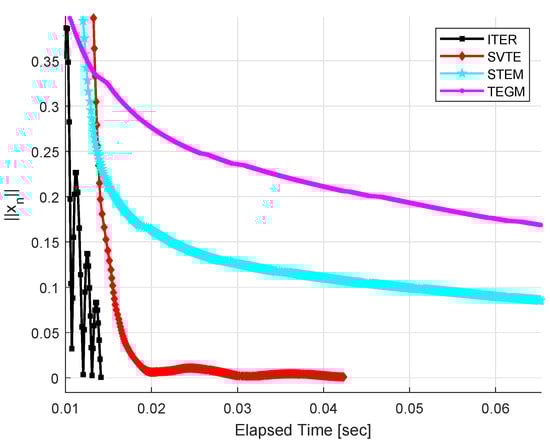
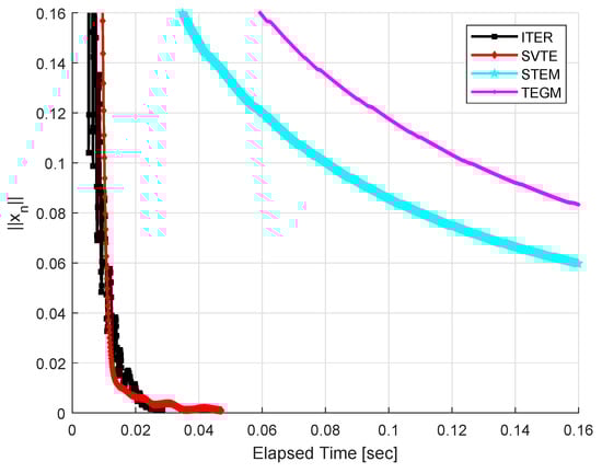
Let $\mathcal{H}={\mathbb{R}}^m$ with inner product $\langle ·,·\rangle :\mathcal{H}\times \mathcal{H}\to \mathbb{R}$ defined by ${\displaystyle \langle x,y\rangle :=\sum _{j=1}^m{x}_j{y}_j}$. The feasible set $\mathcal{C}$ is given by $\mathcal{C}=\{x\in {\mathbb{R}}^m:∥x∥\le 1\}.$ Take the operator $\mathcal{A}\left(x\right):=Mx+p,$ where $M=B{B}^T+D,$ and B is an $m\times m$ matrix, D is an $m\times m$ diagonal matrix, whose diagonal entries are nonnegative, p is a vector in ${\mathbb{R}}^m$. It is clear that $\mathcal{A}$ is monotone and L-Lipschitz-continuous with $L=∥M∥$. Similarly, take the operator $\mathcal{F}\left(x\right):=Qx+q,$ where $Q=N{N}^T+G,$ and N is an $m\times m$ matrix, G is an $m\times m$ diagonal matrix, whose diagonal entries are positive, q is a vector in ${\mathbb{R}}^m$. We can check that $\mathcal{F}$ is h-strongly monotone and k-Lipschitz continuous with $k=∥Q∥$, $h=min\left\{eig\right(Q\left)\right\},$ where eig$\left(Q\right)$ represents all eigenvalues of Q. Let $p=q=0$, $\mathrm{\Psi }(x,y)=y^2+3xy-4x^2$ for all $x,y\in {\mathbb{R}}^m$, $\mathrm{\Phi }\left(x\right)=x^2$ and $g\left(x\right)=\frac{99}{100}x$ for all $x\in {\mathbb{R}}^m$. It is easy to see that $K_{r}x=\frac{x}{1+7r}$ and the unique solution to the VOGME (10) is 0.

We choose the stepsize $r=\frac{9}{10∥A∥}$ for TEGM and $r_n=\frac{9min\left\{eig\right(Q\left)\right\}}{10{∥A∥}^2}$ for IMR. Take ${\alpha }_n={(n+1)}^{-0.8}$, $r_1=\frac{1}{3}$, and $\nu =\frac{9}{10}$ for STEM; ${\alpha }_n={(n+1)}^{-0.8}$, ${ϵ}_n={(n+1)}^{-0.7}$, ${\sigma }_n={(n+1)}^{-2}$, $r_1=\frac{1}{3}$, $\varrho =1$ and $\nu =\frac{9}{10}$ for SVTE; ${ϵ}_n={(n+1)}^{-0.7}$ and $\varrho =1$ for IMR; ${ϵ}_n={(n+1)}^{-0.7}$, ${\sigma }_n={(n+1)}^{-2}$, $r_1=\frac{1}{3}$, $\varrho =1$ and $\nu =\frac{9}{10}$ for ITER. Set $∥x_n∥<{10}^{-3}$ as stopping criterion and the initial values $x_0,x_1$ are generated randomly in $(-6,6)$. Figure 1 and Figure 2 describe the numerical results.

Example 2.

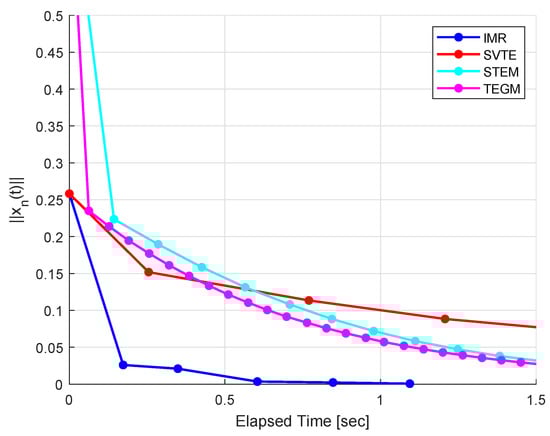
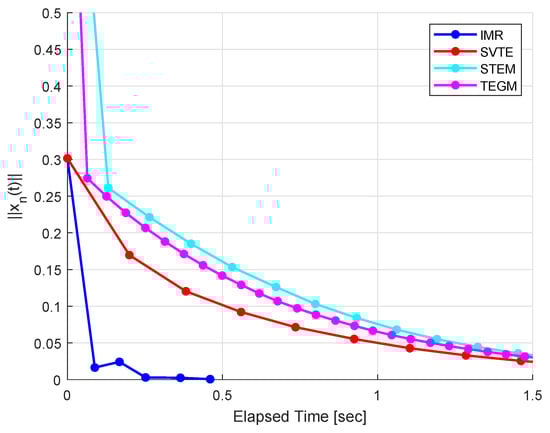
We consider an example that appears in the infinite dimensional Hilbert space $\mathcal{H}=L^2\left([0,1]\right)$ with inner product $\langle x,y\rangle ={\int }_0^{1}x\left(t\right)y\left(t\right)dt$ and the induced norm $∥x∥={\left({\int }_0^1{x}^2\left(t\right)dt\right)}^{1/2}$. The feasible set $\mathcal{C}$ is given by $\mathcal{C}=\{x\in L^2\left([0,1]\right):∥x∥\le 1\}.$ Let $\mathrm{\Psi }:\mathcal{H}\times \mathcal{H}\to \mathbb{R}$ be given by $\mathrm{\Psi }(x,y)=y^2+3xy-4x^2$ for all $x,y\in \mathcal{H}$, $\mathrm{\Phi }\left(x\right)=x^2$, $\mathcal{A}x=x$, $\mathcal{F}x=\frac{1}{2}x$ and $g\left(x\right)=\frac{99}{100}x$ for all $x\in \mathcal{H}$. It is easy to verify that 0 is the unique solution to the VOGME (10). We choose the stepsize $r=\frac{9}{10∥A∥}$ for TEGM and $r_n=\frac{9}{10}$ for IMR. Our parameters are the same as in Example 1. Use $∥x_n∥<{10}^{-3}$ as stopping criterion and the numerical results are reported in Figure 3 and Figure 4.

5. Conclusions

This work presents two alternative regularization methods for finding a solution of the variational inequality problem over the set of solutions of the generalized mixed equilibrium problem. These methods can be viewed as an improvement of Tseng’s extragradient method and the regularization method. We show that the iterative process generated by proposed methods converge strongly to solutions of above bilevel problems. The theoretical results are also confirmed by two numerical examples.

References

- Combettes, P.L.; Hirstoaga, S.A. Equilibrium programming in Hilbert spaces. J. Nonlinear Convex Anal. 2005, 6, 117–136. [Google Scholar]
- Tan, B.; Qin, X.; Yao, J.C. Strong convergence of self-adaptive inertial algorithms for solving split variational inclusion problems with applications. J. Sci. Comput. 2021, 87, 20. [Google Scholar] [CrossRef]
- Yao, Y.; Cho, Y.J.; Liou, Y.C. Algorithms of common solutions for variational inclusions, mixed equilibrium problems and fixed point problems. Eur. J. Oper. Res. 2011, 212, 242–250. [Google Scholar] [CrossRef]
- Song, Y.L.; Bazighifan, O. A New Alternative Regularization Method for Solving Generalized Equilibrium Problems. Mathematics 2022, 10, 1350. [Google Scholar] [CrossRef]
- Song, Y.L. Hybrid Inertial Accelerated Algorithms for Solving Split Equilibrium and Fixed Point Problems. Mathematics 2021, 9, 2680. [Google Scholar] [CrossRef]
- Jolaoso, L.O.; Karahan, I. A general alternative regularization method with line search technique for solving split equilibrium and fixed point problems in Hilbert spaces. Comput. Appl. Math. 2020, 39, 150. [Google Scholar] [CrossRef]
- Korpelevich, G.M. An extragradient method for finding saddle points and for other problems. Matecon 1976, 12, 747–756. [Google Scholar]
- Tan, B.; Qin, X. Self adaptive viscosity-type inertial extragradient algorithms for solving variational inequalities with applications. Math. Model. Anal. 2022, 27, 41–58. [Google Scholar] [CrossRef]
- Fichera, G. Sul problema elastostatico di Signorini con ambigue condizioni al contorno. Atti Accad. Naz. Lincei Rend. Cl. Sci. Fis. Mat. Nat. 1963, 34, 138–142. [Google Scholar]
- Hartman, P.; Stampacchia, G. On some nonlinear elliptic differential functional equations. Acta Math. 1966, 115, 271–310. [Google Scholar] [CrossRef]
- Bnouhachem, A.; Chen, Y. An iterative method for a common solution of generalized mixed equilibrium problem, variational inequalities and hierarchical fixed point problems. Fixed Point Theory Appl. 2014, 2014, 155. [Google Scholar] [CrossRef]
- Bazighifan, O. An approach for studying asymptotic properties of solutions of neutral differential equations. Symmetry 2020, 12, 555. [Google Scholar] [CrossRef]
- Bazighifan, O.; Kumam, P. Oscillation theorems for advanced differential equations with p-Laplacian like operators. Mathematics 2020, 8, 821. [Google Scholar] [CrossRef]
- Xu, H.K. Iterative algorithm for nonlinear operators. J. Lond. Math. Soc. 2002, 2, 240–256. [Google Scholar] [CrossRef]
- Goebel, K.; Reich, S. Uniform Convexity, Hyperbolic Geometry, and Nonexpansive Mappings; Marcel Dekker, Inc.: New York, NY, USA, 1984. [Google Scholar]
- Xu, H.K. Viscosity approximation methods for nonexpansive mappings. J. Math. Anal. Appl. 2004, 298, 279–291. [Google Scholar] [CrossRef]
- Antipin, A.S. On a method for convex programs using a symmetrical modification of the Lagrange function. Ekon. Mat. Metody. 1976, 12, 1164–1173. [Google Scholar]
- Tseng, P. A modified forward-backward splitting method for maximal monotone mapping. SIAM J. Control Optim. 2000, 38, 431–446. [Google Scholar] [CrossRef]
- Bauschke, H.; Combettes, P. A weak-to-strong convergence principle for feje´r-monotone methods in Hilbert spaces. Math. Oper. Res. 2001, 26, 248–264. [Google Scholar] [CrossRef]
- Yang, J.; Liu, H. Strong convergence result for solving monotone variational inequalities in Hilbert spaces. Numer. Algor. 2019, 80, 741–752. [Google Scholar] [CrossRef]
- Thong, D.V.; Li, X.H.; Dong, Q.L.; Cho, Y.J.; Rassias, T.M. A projection and contraction method with adaptive step sizes for solving bilevel pseudo-monotone variational inequality problems. Optimization 2020, 71, 2073–2096. [Google Scholar] [CrossRef]
- Tan, B.; Liu, L.; Qin, X. Self adaptive inertial extragradient algorithms for solving bilevel pseudomonotone variational inequality problems. Jpn. Ind. Appl. Math. 2021, 38, 519–543. [Google Scholar] [CrossRef]
- Song, Y.; Bazighifan, O. Regularization Method for the Variational Inequality Problem over the Set of Solutions to the Generalized Equilibrium Problem. Mathematics 2022, 10, 2443. [Google Scholar] [CrossRef]
- Moudafi, A. Proximal methods for a class of bilevel monotone equilibrium problems. J. Glob. Optim. 2010, 47, 287–292. [Google Scholar] [CrossRef]
- Cottle, R.W.; Yao, J.C. Pseudo-monotone complementarity problems in Hilbert space. J. Optim. Theory Appl. 1992, 75, 281–295. [Google Scholar] [CrossRef]
Publisher’s Note: MDPI stays neutral with regard to jurisdictional claims in published maps and institutional affiliations. |
© 2022 by the authors. Licensee MDPI, Basel, Switzerland. This article is an open access article distributed under the terms and conditions of the Creative Commons Attribution (CC BY) license (https://creativecommons.org/licenses/by/4.0/).