Unbiased Identification of Fractional Order System with Unknown Time-Delay Using Bias Compensation Method

Abstract

In the field of engineering, time-delay is a typical occurrence. In reality, the inner dynamics of many industrial processes are impacted by delay or after-effect events. This paper discusses the identification of continuous-time fractional order system with unknown time-delay using the bias compensated least squares algorithm. The basic concept is to remove the imposed bias by including a correction term into the least squares estimations. The suggested approach makes a significant contribution by the estimation, iteratively, of fractional order system coefficients as well as the orders and the time-delay using a nonlinear optimization algorithm. The main advantage of this method is to provide a simple and powerful algorithm with good accuracy. The suggest method performances are assessed through two numerical examples.

1. Introduction

In recent years, the use of fractional calculus has become increasingly widespread. In fact, fractional order systems have received great interest and relevance [1,2,3,4,5,6]. Examples can be found in a variety of scientific fields: in mechanics, such as dynamic models that govern the relaxation of water on a porous dyke [7], dielectric materials [8], modeling of rotor skin effect in induction machines [9], thermal diffusive phenomena [10,11,12,13], traffic in information networks [14], and muscle relaxation in biology systems [15]. The feature of fractional order differentiation is that it supplies a precious instrument for modeling real-world processes with long memory, interactions, and hereditary properties, in contrast to integer order differentiation, where such properties are neglected [16]. For these reasons, researchers are interested in modeling with fractional order differential equations [17,18].

The fractional order system identification is the foundation of the stability analysis and controller design for fractional order systems. In the literature, various methodologies for the identification of systems can be found using fractional calculus: Battagalia et al. [19] have proposed a fractional model which produces the transient thermal behavior of a system. The simplified refined instrumental variable (SRIV) method has been extended to identify both differentiation orders and coefficients of the fractional system by Malti et al. in [20]. In Ref. [21], a lithium-ion battery has been identified using the fractional state space model. Recently, in 2015, the fractional closed loop system identification emerged as an important research area. Thus, an electronic real system has been estimated in closed loop experiments in [22]. The parametric identification of fractional order nonlinear systems has been studied by Mani et al. as indicated in [23]. In Ref. [24] coefficients and fractional orders based on block pulse functions (BPF) through a two-stage algorithm has been established.

All the aforementioned work involved fractional order systems without time-delay. On the other hand, most realistic physical processes contain a time-delay. Therefore, the identification of fractional order systems with an unknown time-delay is still a challenging problem due to difficulty in formulation caused. It plays an important role in the fractional order signal processing, stability theories, and fractional order control methods [2,25]. However, at present, only a limited number of methods have been extended to identify the fractional order time-delay systems. A brief review is presented in this paragraph. The problem of identifying a fractional order transfer function with time-delay was initiated in 2010 by Peng et al. [2].

In this work, the optimal fractional derivative order and the time-delay of the transfer function model are found using harmony search, while the coefficients are obtained by solving linear least squares problems. In 2011, a frequency domain subspace identification of commensurate fractional order input time-delay systems has been established in [26]. Subsequently, the system identification problem of a Multi-Input-Multi-Output (MIMO) fractional order system with delay in state is studied in [27]. Moreover, an identification algorithm which combines the subspace method and a simulated annealing algorithm and is based on the instrumental variables method has been properly extended to handle the identification of the fractional time-delay systems in [28]. Then, Ref. [29] establishes parameter and delay estimation of fractional order models from step response. In this work, supposing that the fractional orders were known, the authors have presented an integral equation approach for fractional order system modeling. The block pulse functions (BPF) integration operational matrix was combined with the interior point algorithm to estimate the model parameters [30]. Then, utilizing polynomial modulating functions, Gao et al. have proposed a system identification method with measurements noise compensation for fractional order systems with a known delay [31]. Thereafter, a recursive identification of a MIMO fractional order Hammerstein model with time-delay is presented in [32]. Afterwords, a novel approach of fractional order time-delay system modeling based on Haar wavelet has been elaborated in [33]. In 2019, the time-domain identification of one non-integer order plus time-delay models from step response measurements was developed in [34]. More recently, coefficients and delay estimation of the general form of fractional order systems using non-ideal step inputs is detailed in [35]. Lately, in 2022, sin et al. have proposed a new method based on BPF to identify fractional order time-delay systems. Firstly, the operational matrices of BPF for fractional integral and time-delay operators are derived. Then, these operational matrices are applied to convert the fractional order system with time-delay to an algebraic equation. Finally, the system’s parameters and the time-delay are all simultaneously estimated through minimizing a quadric error function [36]. The major drawbacks of this work are that, firstly, the BPF are fixed values in their definition interval, which means that an error is produced when their integration operational matrices are used to convert a fractional order time-delay system into an algebraic equation. In addition, the initial conditions are treated as extra parameters and identified simultaneously with the system parameters, which complicates the identification procedure and can lead to inaccurate results. More importantly, the outputs of engineering systems are often noisy, which greatly affects the consistency of parameter identification.

According to the aforementioned investigations, the primary aspect of this research is first to supply an efficient method to estimate the parameters, namely both the coefficients, the differentiation orders and the time-delay. Firstly, when the differentiation orders and the time-delay are assumed to be known, the fractional order bias compensated least squares ($fbcls$) method, is applied, which is well-known for its conceptual clarity and efficacy in the disciplines of identification and control theory [37,38]. To start this method, firstly, the parameters vector estimations are derived from the fractional order least squares $\left(fols\right)$ method mixed with the state variable filter approach. Secondly, in order to establish estimation consistency, the bias created by least squares parameter estimations is removed. Furthermore, a specific aspect of fractional differential equation modeling is the determination of differentiation orders. This task is too tricky because the order of the model is updated and the optimization problem is nonlinear when minimizing the output error criterion. Therefore, the $fbcls$ method is extended to estimate both the parameters and the fractional orders differentiation. Identification is even more difficult when working with a time-delay system as the total number of parameters increases. To analyze the statistical properties of our new algorithm, Monte Carlo simulation analysis is suggested.

The remainder of this paper is organized as follows. In Section 2, the fractional order differentiation and the description of the fractional order system with time-delay are introduced. The parameter identification technique based on the least squares method and the bias correction procedure is proposed in Section 3. In Section 4, the effectiveness of the proposed method is verified by numerical simulations. Finally, conclusions are drawn in Section 5.

2. Preliminaries

2.1. Fractional Order Differentiation

Three commonly used definitions for the fractional order differentiation are Grünwald-Letnikov (G-L), Riemann-Liouville (R-L), and Caputo definitions [39]. In this paper Grünwald-Letnikov will be used to implement fractional operators:

Definition 1.

The Grünwald-Letnikov derivative approximation of the order α of function $f\left(t\right)$ is described as

$${}_{GL}^{}{D}_{0,t}^{\alpha }f\left(t\right)\simeq \frac{1}{h^{\alpha }}\sum _{k=0}^{⌊\frac{t}{h}⌋}{\left(-1\right)}^k\left(\begin{array}{c}\alpha \hfill \\ k\hfill \end{array}\right)f\left(t-kh\right),\forall t\in {\mathbb{R}}_{+}^{\ast },$$

(1)

where h is the sampling period and $\left(\begin{array}{c}\alpha \hfill \\ k\hfill \end{array}\right)$ is the Newton’s binomial generalized to fractional orders.

2.2. Fractional Order System with Time-Delay Description

For subsequent use, we introduce a brief description of Continuous-Time (CT) fractional order system with time-delay. Let us consider a linear time invariant Single-Input-Single-Ouput (SISO) time-delay system where the input $u\left(t\right)$ and the output $y\left(t\right)$ of the plant are connected by the following differential equation

$$\sum _{n=0}^N{a}_n{\mathrm{D}}^{{\alpha }_n}y\left(t\right)=\sum _{m=0}^M{b}_m{\mathrm{D}}^{{\beta }_m}u\left(t-\tau \right),$$

(2)

where ${\left.a_n\right|}_{n=0:N},{\left.b_m\right|}_{m=0:M}$ are the linear constant coefficients; $({\alpha }_n,{\beta }_m)\in {\mathbb{R}}^{+}$ are the fractional orders and $\tau$ denotes the time-delay.

If all of the differentiation orders ${\alpha }_n$ and ${\beta }_m$ are multiple integers of the same order $\upsilon$, the differential equation is said to be with commensurate order. It may be phrased as follows in this case

$$\sum _{i=0}^{n_a}{a}_i{\mathrm{D}}^{i\upsilon }y\left(t\right)=\sum _{j=0}^{n_b}{b}_j{\mathrm{D}}^{j\upsilon }u\left(t-\tau \right),$$

(3)

where $\upsilon$ denotes the commensurate order.

In order to describe the dynamical behavior of systems, the Laplace transform is often used. Expression (4) gives the Laplace transform of the Equation (3) taking into account zero initial conditions

$$\begin{array}{ccc}\hfill G\left(s\right)& =& \frac{B\left(s\right)}{A\left(s\right)}=\frac{{\displaystyle \sum _{j=0}^{n_b}}{b}_j{s}^{j\upsilon }}{{\displaystyle \sum _{i=0}^{n_a}}{a}_i{s}^{i\upsilon }}{e}^{-\tau s}.\hfill \end{array}$$

(4)

2.3. Problem Formulation

The system considered in this paper is presented as follows:

$${\mathcal{G}}_0:\left\{\begin{array}{c}\begin{array}{c}{\mathcal{A}}_0\left(p\right)\chi \left(t\right)={\mathcal{B}}_0\left(p\right)u(t-\tau ),\end{array}\\ y\left(t\right)=\chi \left(t\right)+e\left(t\right).\end{array}\right.$$

(5)

Without loss of generality, $a_0$ is taken equal to 1. $p=\frac{d}{dt}$ denotes the differentiation operator. $u(t-\tau )$, $\chi \left(t\right)$ and $y\left(t\right)$ are, respectively, the delayed input signal, the system noise-free output signal, and the measured output signal. $e\left(t\right)$ is an additive zero-mean white Gaussian noise corrupting the output signal and assumed to be uncorrelated with the input signal.

${\mathcal{A}}_0\left(p\right)$, ${\mathcal{B}}_0\left(p\right)$, are polynomials in p of degree $n_a,n_b$ represented as:

$$\left\{\begin{array}{c}{\mathcal{A}}_0\left(p\right)=1+{\displaystyle \sum _{i=1}^{n_a}}{a}_i{p}^{i\upsilon },\\ {\mathcal{B}}_0\left(p\right)={\displaystyle \sum _{j=0}^{n_b}}{b}_j{p}^{j\upsilon }.\end{array}\right.$$

(6)

Consider the parameterized model describing the system $\mathcal{G}$, presented by the following equation

$$\mathcal{M}:y\left(t\right)=-\sum _{i=1}^{n_a}{a}_i{D}^{i\upsilon }y\left(t\right)+\sum _{j=0}^{n_b}{b}_j{D}^{j\upsilon }u(t-\tau )+\epsilon \left(t\right).$$

(7)

where

$$\epsilon \left(t\right)=e\left(t\right)+\sum _{i=1}^{n_a}{a}_i{D}^{i\upsilon }e\left(t\right).$$

(8)

The following linear regression form explains the behavior of the fractional system’s inputs and outputs.

$$y\left(t\right)={\Phi }^T\left(t\right)\rho +\epsilon \left(t\right),$$

(9)

where $\rho$ represents the parameters vector and $\Phi$ is the regression vector, which are defined, respectively, as follows

$$\rho =\left[\begin{array}{cccccc}{a}_1,& \dots ,& a_{n_a},& b_0,& \dots ,& b_{n_b}\end{array}\right]\in {\mathbb{R}}^{(n_a+n_b+1)},$$

(10)

$$\begin{array}{c}\hfill {\Phi }^T\left(t\right)=\left[\begin{array}{ccc}-D^{\upsilon }y\left(t\right),& \dots ,& -D^{n_a\upsilon }y\left(t\right),\end{array}\right.\left.\begin{array}{ccc}u\left(t-\tau \right),& \dots ,& D^{n_b\upsilon }u\left(t-\tau \right)\end{array}\right].\end{array}$$

(11)

and $\epsilon \left(t\right)$ is the residual error.

It should be pointed out that the inevitable direct fractional differentiation of noisy output is a major problem in the fractional system identification, which leads to inaccurate estimates. Therefore, the use of a state variable filter (svf) proposed in [18] is absolutely necessary.

Suppose the svf specified by the subsequent equation

$$L_{\upsilon }\left(p\right)=p^{\upsilon }{\left(\frac{\varpi }{\varpi +p}\right)}^{\eta },$$

(12)

where $\upsilon$ is the fractional order differentiation, the order $\eta$ is an integer chosen such that $\eta >n_a\upsilon$ and $\varpi$ denotes the filter cut-off frequency.

The filtered input and output signals $u_f\left(t\right)$ and $y_f\left(t\right)$ are determined as follows:

$$\left\{\begin{array}{c}{D}^{j\upsilon }{u}_f\left(t\right)=L_{j\upsilon }\left(p\right)u\left(t\right),\hfill \\ D^{i\upsilon }{y}_f\left(t\right)=L_{i\upsilon }\left(p\right)y\left(t\right).\hfill \end{array}\right.$$

(13)

So, the regression vector containing the filtered signals is represented as follows

$$\begin{array}{c}{\Phi }_f^T\left(t\right)=\left[\begin{array}{ccc}-D^{\upsilon }{y}_f\left(t\right),& \dots ,& -D^{n_a\upsilon }{y}_f\left(t\right),\end{array}\right.\hfill \\ \left.\begin{array}{ccc}{u}_f\left(t-\tau \right),& \dots ,& D^{n_b\upsilon }{u}_f\left(t-\tau \right)\end{array}\right].\hfill \end{array}$$

Using the filtered input and output signals, Equation (9) can be reformulated as

$$y_f\left(t\right)={\Phi }_f^T\left(t\right)\rho +{\epsilon }_f\left(t\right),$$

(14)

where ${\epsilon }_f\left(t\right)$ is expressed as follows

$${\epsilon }_f\left(t\right)=\sum _{i=0}^{n_a}{a}_i{L}_{i\upsilon }e\left(t\right).$$

(15)

In reality, the purpose of this research is to identify the fractional system with an unknown time-delay from $N_s$ samples of the input and noisy output signals using the bias compensated least squares approach combined with a nonlinear optimization algorithm.

3. Fractional Order System Identification

The system identification procedure involves constructing an appropriate model from input/output data. System identification is not simply a method for constructing a model from collected data. However, a solid experimental design and prior information, if available, are required for its use. In frequency domain and time domain system identification, a fractional model structure was adopted [18,40,41]. Literature predominantly uses two groups of methodologies: equation error-based methods and output error-based methods. Numerous actual systems are capable of being represented using the fractional model: Electrode-electrolyte polarization, diffusion systems: electro-chemistry, heat transfer, and electromagnetism, nuclear reactor, charge estimation of lead acid battery, semi-infinite thermal system, thermal diffusion in a wall [16,17].

In this section, the identification of fractional order systems with an unknown time-delay is discussed. The main objective is to identify the coefficients as well as the fractional differentiation orders and the time-delay. There are two significant steps during the presented new identification algorithm:

Step 1: suppose that the commensurate order $\upsilon$ and time-delay $\tau$ are known, and the fractional bias compensated least squares $\left(fbcls\right)$ method is proposed to initialize the coefficients vector.

Step 2: the nonlinear optimization method based on the Levenberg-Marquardt algorithm is introduced to estimate, namely, coefficients, the differentiation order, and the time-delay.

3.1. Compensation for Measurement Noises Existing in the Output Signal

It is assumed that the fractional commensurate order $\upsilon$ and the time-delay $\tau$ are already known, and our goal is to estimate just the fractional differential equation coefficients. Initially, this section describes the fractional order least squares $\left(fols\right)$ approach for identifying the fractional order systems with time-delay.

Let ${\epsilon }_f\left(t\right)$ the filtered equation error defined as

$${\epsilon }_f\left(t\right)=y_f\left(t\right)-{\Phi }_f^T\left(t\right)\rho .$$

(16)

Consider the ${\widehat{\rho }}_{fols}\left(N_s\right)$ as the estimated vector of $\rho$ generated by minimizing the 2-norm of the below criterion function

$$V_{N_s}\left({\widehat{\rho }}_{fols}\left(N_s\right)\right)=\frac{1}{N_s}\sum _{k=1}^{N_s-1}{\epsilon }_f^2\left(t_k,{\widehat{\rho }}_{fols}\right).$$

(17)

Thus, the $fols$ estimate of $\rho$ is obtained by the following equation

$$\begin{array}{ccc}\hfill {\widehat{\rho }}_{fols}\left(N_s\right)& =& {\left(\sum _{k=0}^{N_s-1}{\Phi }_f\left(t_k\right){\Phi }_f^T\left(t_k\right)\right)}^{-1}\left(\sum _{k=0}^{N_s-1}{\Phi }_f\left(t_k\right)y_f\left(t_k\right)\right)\hfill \\ & =& R_{{\Phi }_f{\Phi }_f}^{-1}{R}_{{\Phi }_f{\epsilon }_f}^{},\hfill \end{array}$$

(18)

where the auto-covariance matrix $R_{{\Phi }_f{\Phi }_f}$ and the cross-covariance $R_{{\Phi }_f{y}_f}$ are given by the following expressions:

$$R_{{\Phi }_f{\Phi }_f}=\sum _{k=0}^{N_s-1}{\Phi }_f\left(t_k\right){\Phi }_f^T\left(t_k\right).$$

(19)

$$R_{{\Phi }_f{y}_f}=\sum _{k=0}^{N_s-1}{\Phi }_f\left(t_k\right)y_f\left(t_k\right).$$

(20)

Theorem 1.

Consider the consistency property of the $fols$ estimator, i.e., the behavior estimates of the parameters when the number of data $N_s$ tends to infinity:

$$\begin{array}{ccc}\hfill \underset{N_s\to \infty }{\lim }{\widehat{\rho }}_{fols}\left(N_s\right)& =& \rho +R_{{\Phi }_f{\Phi }_f}^{-1}{R}_{{\Phi }_f{\epsilon }_f}\hfill \\ & =& \rho +B_{\rho }.\hfill \end{array}$$

(21)

Under the sufficiently exciting condition, the Gaussian noise $e\left(t\right)$ is independent with the input signal $u\left(t\right)$, the estimation error can be expressed as

$$\begin{array}{ccc}\hfill B_{\rho }& =& R_{{\Phi }_f{\Phi }_f}^{-1}{R}_{{\Phi }_f{\epsilon }_f}\hfill \\ & =& R_{{\Phi }_f{\Phi }_f}^{-1}\Xi R_{y_f{\epsilon }_f},\hfill \end{array}$$

(22)

where the matrix $\Xi =\left[\begin{array}{c}{I}_{n_a}\\ 0_{n_b}\end{array}\right]\in {\mathbb{R}}^{\left((n_a+n_b+1)\right)\times \left(n_a\right)}$.

Proof. 

Based on the Equation (14) the $fols$ estimator (18) can be rewritten as the following form

$$\begin{array}{ccc}\hfill {\widehat{\rho }}_{fols}\left(N_s\right)& =& {\left(\sum _{k=0}^{N_s-1}{\Phi }_f\left(t_k\right){\Phi }_f^T\left(t_k\right)\right)}^{-1}\left(\sum _{k=0}^{N_s-1}{\Phi }_f\left(t_k\right)\left({\Phi }_f^T\left(t_k\right)\rho +{\epsilon }_f\left(t_k\right)\right)\right)\hfill \end{array}$$

$$\begin{array}{ccc}& =& \rho +{\left(\sum _{k=0}^{N_s-1}{\Phi }_f\left(t_k\right){\Phi }_f^T\left(t_k\right)\right)}^{-1}\left(\sum _{k=0}^{N_s-1}{\Phi }_f\left(t_k\right)\left({\epsilon }_f\left(t_k\right)\right)\right)\hfill \end{array}$$

(23)

$$\begin{array}{ccc}& =& \rho +R_{{\Phi }_f{\Phi }_f}^{-1}{R}_{{\Phi }_f{\epsilon }_f}^{}.\hfill \end{array}$$

(24)

It is clear if the input signal $u\left(t\right)$ can sufficiently excite the identified system, the matrix $R_{{\Phi }_f{\Phi }_f}$ is invertible and the bias expression is given by the following equation

$$B_{\rho }=R_{{\Phi }_f{\Phi }_f}^{-1}{R}_{{\Phi }_f{\epsilon }_f},$$

(25)

where $B_{\rho }$ denotes the bias introduced by the $fols$ method.

Note that also the input signal $u\left(t\right)$ is uncorrelated with the noise $e\left(t\right)$; thus, $R_{{\Phi }_f{\epsilon }_f}$ can be rewritten as follows

$$\begin{array}{ccc}\hfill R_{{\Phi }_f{\epsilon }_f}^{}\left(N_s\right)& =& \left[\begin{array}{c}-D^{\upsilon }{y}_f^{}\left(t_k\right){\epsilon }_f\left(t\right)\\ ⋮\\ -D^{n_a\upsilon }{y}_f^{}\left(t_k\right){\epsilon }_f\left(t\right)\\ 0\\ ⋮\\ 0\end{array}\right]\hfill \\ & =& \left[\begin{array}{c}1\\ ⋮\\ 1\\ 0\\ ⋮\\ 0\end{array}\right]R_{y_f{\epsilon }_f}.\hfill \end{array}$$

(26)

Replacing Equation (26) in Equation (23), we get the following equation

$$\begin{array}{ccc}\hfill {\widehat{\rho }}_{fols}\left(N_s\right)& =& \rho +R_{{\Phi }_f{\Phi }_f}^{-1}\Xi R_{y_f{\epsilon }_f}^{}\hfill \\ & =& \rho +B_{\rho }.\hfill \end{array}$$

(27)

Therefore, the bias expression is $B_{\rho }=R_{{\Phi }_f{\Phi }_f}^{-1}\Xi R_{y_f{\epsilon }_f}.$

Obviously, $R_{y_f{\epsilon }_f}$ is different to zero and, thus, the bias estimate $B_{\rho }$ is certainly non-zero. Then, the $fols$ estimator is biased.    □

The second step in our numerical scheme consists in compensating the bias introduced by the $fols$ method $B_{\rho }$ using the $fbcls$ method whose principle is given by the following expression

$$\begin{array}{ccc}\hfill {\widehat{\rho }}_{fbcls}& =& {\widehat{\rho }}_{fols}-B_{\rho }\hfill \\ & =& {\widehat{\rho }}_{fols}-R_{{\Phi }_f{\Phi }_f}^{-1}\Xi R_{y_f{\epsilon }_f}.\hfill \end{array}$$

(28)

The primary challenge with this technique is that the $fols$ method can only supply a single equation to estimate the bias $B_{\rho }$. Therefore, it is essential to find other equations to solve this problem. Basically, the idea of the proposed method is to augment the nominator parameters by $n_a-n_b$ dimensions and the introduced parameters $b_j=0j=\left\{n_b+1,\dots ,n_a+n_b\right\}$. As a result, the augmented model, which is used to get an unbiased estimator, can be represented as follows

$$\begin{array}{c}{y}_f\left(t\right)=-a_1{D}^{\upsilon }{y}_f\left(t\right)-...-a_{n_a}{D}^{n_a\upsilon }{y}_f\left(t\right)\hfill \\ +b_0{u}_f\left(t-\tau \right)+b_1{D}^{\upsilon }{u}_f\left(t-\tau \right)+...+b_{n_a+n_b}{D}^{\left(n_a+n_b\right)\upsilon }{u}_f\left(t-\tau \right).\hfill \end{array}$$

(29)

Moreover, the filtered output signal can be expressed as follows

$$y_f\left(t\right)={\overline{\Phi }}_f^T\left(t\right)\overline{\rho }+{\epsilon }_f\left(t\right),$$

(30)

and the augmented parameters vector is presented by

$$\begin{array}{c}\hfill \overline{\rho }=\left[\begin{array}{cc}\rho & {\overline{b}}^T\end{array}\right],\end{array}$$

(31)

where the vector ${\overline{b}}^T$ is defined as follows

$$\begin{array}{ccc}\hfill {\overline{b}}^T& =& \left[\begin{array}{ccc}{b}_{n_b+1}& \dots & b_{n_b+n_a}\end{array}\right]\hfill \\ & =& \left[\begin{array}{ccc}0& \dots & 0\end{array}\right]\in {\mathbb{R}}^{n_a}.\hfill \end{array}$$

(32)

The augmented regression vector ${\overline{\Phi }}_f^T\left(t_k\right)$ is given by the following expression

$$\begin{array}{ccc}\hfill {\overline{\Phi }}_f^T\left(t_k\right)& =& \left[\begin{array}{cccccc}-D^{\upsilon }{y}_f\left(t_k\right)& \dots & -D^{n_a\upsilon }{y}_f\left(t_k\right)& u_f\left(t_k-\tau \right)& \dots & D^{\left(n_a+n_b\right)\upsilon }{u}_f\left(t_k-\tau \right)\end{array}\right]\hfill \\ & =& \left[\begin{array}{cc}{\Phi }_f^T\left(t_k\right)& {\overline{u}}_f^T\left(t_k\right)\end{array}\right],\hfill \end{array}$$

(33)

where the vector ${\overline{u}}_f^T\left(t\right)$ is defined by

$${\overline{u}}_f^T\left(t_k\right)=\left[\begin{array}{ccc}{D}^{(n_b+1)\upsilon }{u}_f\left(t_k-\tau \right)& \dots & D^{(n_a+n_b)\upsilon }{u}_f\left(t_k-\tau \right)\end{array}\right].$$

(34)

Hence, the augmented estimator $fols$ is computed according to

$$\begin{array}{ccc}\hfill {\widehat{\overline{\rho }}}_{fols}& =& \overline{\rho }+R_{{\overline{\Phi }}_f{\overline{\Phi }}_f}^{-1}\overline{\Xi }{R}_{y_f{\epsilon }_f},\hfill \end{array}$$

(35)

where the matrix $\overline{\Xi }$ is given by the following equation

$$\overline{\Xi }=\left[\begin{array}{c}{I}_{n_a}\\ 0_{\left(n_a+n_b\right)}\end{array}\right]\in {\mathbb{R}}^{\left((2n_a+n_b+1)\right)\times \left(n_a\right)}.$$

(36)

Let the augmented auto-covariance matrix decompose $R_{{\overline{\Phi }}_f{\overline{\Phi }}_f}$ as follows

$$R_{{\overline{\Phi }}_f{\overline{\Phi }}_f}=\left[\begin{array}{cc}{R}_{{\overline{\Phi }}_f{\overline{\Phi }}_f}& R_{{\Phi }_f{\overline{u}}_f}\\ R_{{\Phi }_f{\overline{u}}_f}& R_{{\overline{u}}_f{\overline{u}}_f}\end{array}\right],$$

(37)

and its inverse $R_{{}_{{\overline{\Phi }}_f{\overline{\Phi }}_f}}^{-1}$ can be expressed as

$$R_{{\overline{\Phi }}_f{\overline{\Phi }}_f}^{-1}=\left[\begin{array}{cc}{R}_{{}_{{\Phi }_f{\Phi }_f}}^{-1}+\beta & -R_{{\Phi }_f{\Phi }_f}^{-1}{R}_{{\Phi }_f{\overline{u}}_f}{X}^{-1}\\ -X^{-1}{R_{{\Phi }_f{\overline{u}}_f}}^T{R}_{{}_{{\Phi }_f{\Phi }_f}}^{-1}& X^{-1}\end{array}\right].$$

(38)

where $X=R_{{\overline{u}}_f{\overline{u}}_f}-R_{{\Phi }_f{\overline{u}}_f}^T{R}_{{}_{{\Phi }_f{\Phi }_f}}^{-1}{R}_{{\Phi }_f{\overline{u}}_f}$ and $\beta =R_{{}_{{\Phi }_f{\Phi }_f}}^{-1}{R}_{{\Phi }_f{\overline{u}}_f}{X}^{-1}{R}_{{\Phi }_f{\overline{u}}_f}^T{R}_{{\Phi }_f{\Phi }_f}^{-1}$. Replacing Equation (38) in Equation (35), we get

$$\begin{array}{ccc}\hfill \widehat{\overline{b}}& =& -X^{-1}{R}_{{\Phi }_f{\overline{u}}_f}^T{R}_{{}_{{\Phi }_f{\Phi }_f}}^{-1}{R}_{{}_{{\Phi }_f{y}_f}}^{}+X^{-1}{R}_{{\overline{u}}_f{y}_f}\hfill \\ & =& -X^{-1}\left(R_{{\Phi }_f{\overline{u}}_f}^T{\widehat{\rho }}_{fols}\left(N_s\right)-R_{{\overline{u}}_f{y}_f}\right).\hfill \end{array}$$

(39)

As $\overline{b}=0$ and using Equations (31), (32) and (38), it is obvious that

$$\begin{array}{c}\widehat{\overline{b}}=\overline{b}-X^{-1}{R}_{{\Phi }_f{\overline{u}}_f}^T{R}_{{}_{{\Phi }_f{\Phi }_f}}^{-1}\Xi R_{{}_{y_f{\epsilon }_f}}^{}\\ =-X^{-1}{R}_{{\Phi }_f{\overline{u}}_f}^T{R}_{{}_{{\Phi }_f{\Phi }_f}}^{-1}\Xi R_{{}_{y_f{\epsilon }_f}}^{}.\end{array}$$

(40)

In addition, equalize the two expressions (39) and (40) results

$$-X^{-1}{R}_{{\Phi }_f{\overline{u}}_f}^T{R}_{{}_{{\Phi }_f{\Phi }_f}}^{-1}\Xi R_{{}_{y_f{\epsilon }_f}}^{}=-X^{-1}\left(R_{{\Phi }_f{\overline{u}}_f}^T{\widehat{\rho }}_{fols}\left(N_s\right)-R_{{\overline{u}}_f{y}_f}\right).$$

(41)

It is obvious to obtain the expression of $R_{y_f{\epsilon }_f}$ using the Equation (41)

$$R_{y_f{\epsilon }_f}={\left(R_{{\Phi }_f{\overline{u}}_f}^T{R}_{{\Phi }_f{\Phi }_f}^{-1}\Xi \right)}^{-1}\left(R_{{\Phi }_f{\overline{u}}_f}^T{\widehat{\rho }}_{fols}\left(N_s\right)-R_{{\overline{u}}_f{y}_f}\right).$$

(42)

Now, it is easy to calculate the bias estimation $B_{\rho }$ by substituting Equation (42) in the Equation (22)

$${\widehat{B}}_{\rho }=R_{{}_{{\Phi }_f{\Phi }_f}}^{-1}\Xi {\left(R_{{\Phi }_f{\overline{u}}_f}^T{R}_{{}_{{\Phi }_f{\Phi }_f}}^{-1}\Xi \right)}^{-1}\left(R_{{\Phi }_f{\overline{u}}_f}^T{\widehat{\rho }}_{fols}\left(N_s\right)-R{}_{{\overline{u}}_f{y}_f}\right).$$

(43)

Consequently, the $fbcls$ estimator is obtained by the following equation

$$\begin{array}{ccc}\hfill {\widehat{\rho }}_{fbcls}\left(N_s\right)& =& {\widehat{\rho }}_{fols}\left(N_s\right)-B_{\rho }.\hfill \\ \hfill & =& {\rho }_{fols}\left(N_s\right)-R_{{}_{{\Phi }_f{\Phi }_f}}^{-1}\Xi {\left(R_{{\Phi }_f{\overline{u}}_f}^T{R}_{{}_{{\Phi }_f{\Phi }_f}}^{-1}\Xi \right)}^{-1}\hfill \\ & \times & \left(R_{{\Phi }_f{\overline{u}}_f}^T{\widehat{\rho }}_{fols}\left(N_s\right)-R_{{\overline{u}}_f{y}_f}^{}\right).\hfill \end{array}$$

(44)

Convergence Analysis

In this section, we show that the $fbcls$ algorithm is strongly consistent. The main key to establishing the consistency of the $fbcls$ estimator is to demonstrate that the estimation of $R_{y_f{\epsilon }_f}$ is consistent.

Theorem 2.

Consider the proposed $fbcls$ estimator for fractional order system identification with time-delay. We may conclude that there is a coherent convergence of the parameters

$$\underset{N_s\to \infty }{\lim }{\widehat{\rho }}_{fbcls}\left(N_s\right)=\rho .$$

(45)

Proof. 

Recalling that

$$\begin{array}{c}\underset{N_s\to \infty }{\lim }{R}_{y_f{\epsilon }_f}\left(N_s\right)={\left(R_{{\Phi }_f{\overline{u}}_f}^T{R}_{{\Phi }_f{\Phi }_f^{}}^{-1}\Xi \right)}^{-1}\times \\ \left.\left(R_{{\Phi }_f{\overline{u}}_f}^T{\widehat{\rho }}_{fols}\left(N_s\right)-R_{{\overline{u}}_f{y}_f}\right)\right).\end{array}$$

(46)

replacing ${\widehat{\rho }}_{fols}$ by its expression given by the Equation (27), we get

$$\begin{array}{c}\underset{N_s\to \infty }{\lim }{\widehat{R}}_{y_f{\epsilon }_f}\left(N_s\right)={\left(R_{{\Phi }_f{\overline{u}}_f}^T{R}_{{\Phi }_f{\Phi }_f^{}}^{-1}\Xi \right)}^{-1}\times \\ \begin{array}{c}\left(R_{{\Phi }_f{\overline{u}}_f}^T\left(\rho +R_{{\Phi }_f{\Phi }_f}^{-1}\Xi R_{y_f{\epsilon }_f}^{}\right)-R_{{\overline{u}}_f{y}_f}\right).\hfill \end{array}\end{array}$$

(47)

so,

$$\begin{array}{c}\underset{N_s\to \infty }{\lim }{\widehat{R}}_{y_f{\epsilon }_f}\left(N_s\right)={\left(R_{{\Phi }_f{\overline{u}}_f}^T{R}_{{\Phi }_f{\Phi }_f^{}}^{-1}\Xi \right)}^{-1}{R}_{{\Phi }_f{\overline{u}}_f}^T\rho +{\left(R_{{\Phi }_f{\overline{u}}_f}^T{R}_{{\Phi }_f{\Phi }_f^{}}^{-1}\Xi \right)}^{-1}\times \hfill \\ \left(R_{{\Phi }_f{\overline{u}}_f}^T{R}_{{\overline{\Phi }}_f{\overline{\Phi }}_f}^{-1}\Xi \right)R_{y_f{\epsilon }_f}^{}-{\left(R_{{\Phi }_f{\overline{u}}_f}^T{R}_{{\Phi }_f{\Phi }_f^{}}^{-1}\Xi \right)}^{-1}{R}_{{\overline{u}}_f{y}_f}\hfill \\ =R_{y_f{\epsilon }_f}^{}+{\left(R_{{\Phi }_f{\overline{u}}_f}^T{R}_{{\Phi }_f{\Phi }_f^{}}^{-1}\Xi \right)}^{-1}\left(R_{{\Phi }_f{\overline{u}}_f}^T\rho -R_{{\overline{u}}_f{y}_f}\right).\hfill \end{array}$$

(48)

Since the independence between the noise $e\left(t\right)$ and the input signal $u\left(t\right)$, the multiplication both side of the Equation (14) by ${\overline{u}}_f\left(t\right)$ implies that

$$\begin{array}{ccc}\hfill {\overline{u}}_f\left(t\right)y_f\left(t\right)& =& {\overline{u}}_f\left(t\right){\Phi }_f^T\rho +{\overline{u}}_f\left(t\right){\epsilon }_f\left(t\right)\hfill \\ & =& {\overline{u}}_f\left(t\right){\Phi }_f^T\rho .\hfill \end{array}$$

(49)

Consequently,

$$R_{{\overline{u}}_f{y}_f}=R_{{\Phi }_f{\overline{u}}_f\left(t\right)}\rho .$$

(50)

Combining the Equations (50) and (48) and letting $N_s$ tends to infinity, we obtain

$$\underset{N_s\to \infty }{\lim }{\widehat{R}}_{y_f{\epsilon }_f}\left(N_s\right)=R_{y_f{\epsilon }_f}.$$

(51)

According to Equation (51), the estimation of $R_{y_f{\epsilon }_f}$ is asymptotically consistent.

It then follows immediately from (27), (28), and (51). Thus, the result is shown on the following equation

$$\begin{array}{ccc}\hfill \underset{N_s\to \infty }{\lim }{\widehat{\rho }}_{fbcls}\left(N_s\right)& =& \underset{N_s\to \infty }{\lim }{\widehat{\rho }}_{fols}\left(N_s\right)-\underset{N_s\to \infty }{\lim }{R}_{{\overline{\Phi }}_f{\overline{\Phi }}_f}^{-1}\left(N_s\right)\Xi R_{y_f{\epsilon }_f}^{}\left(N_s\right)\hfill \end{array}$$

$$\begin{array}{ccc}& =& \left(\rho +R_{{\overline{\Phi }}_f{\overline{\Phi }}_f}^{-1}\Xi R_{y_f{\epsilon }_f}^{}\right)-R_{{\overline{\Phi }}_f{\overline{\Phi }}_f}^{-1}\Xi R_{y_f{\epsilon }_f}^{}\hfill \end{array}$$

(52)

$$\begin{array}{ccc}& =& \rho .\hfill \end{array}$$

(53)

Thus, we have proved the consistency result.    □

3.2. Output Error Method for Fractional Order System with Unknown Time-Delay (FOSTD-OE)

In essence, the application of the $fbcls$ technique is confined to situations where the fractional orders are expected to be known beforehand. This part describes a strategy for extending the identification method introduced in the preceding section to a more realistic scenario in which fractional orders differentiation are assumed to be unknown and calculated, along with coefficients. It is based on the combination of the $fbcls$ method for coefficient estimation and a nonlinear algorithm for optimization of the differentiation order and the time-delay.

First of all, set $\rho$ the parameter vector as follows

$$\rho =\left[\begin{array}{cccccccc}{a}_1,& \dots ,& a_n,& b_0,& \dots ,& b_m,& \upsilon ,& \tau \end{array}\right].$$

(54)

The challenge of identifying parameters is represented as a functional minimization. Therefore, the primary objective of this approach is to reduce the residual error relative to $\upsilon$ and $\tau$. In addition, the comparable order is updated repeatedly using the Levenberg-Marquardt algorithm during the computing phase. The quadratic criterion is, therefore, defined as follows

$$J\left(\widehat{\rho }\right)=\frac{1}{2}{∥\epsilon \left(t\right)∥}_2,$$

(55)

where $\epsilon \left(t\right)$ is the output error defined by

$$\epsilon \left(t\right)=y\left(t\right)-\widehat{y}\left(t\right)$$

(56)

This iterative algorithm calculates the fractional vector parameters ${\rho }^{iter+1}$ at the iteration $iter+1$. The proposed algorithm is named the Fractional System with Time-Delay Output Error $(FSTD-OE)$ algorithm and is described in the Algorithm 1.

Algorithm 1$FSTD-OE$ algorithm

Data$\left\{\begin{array}{cc}u{}_f\left(t\right),& \left.y_f\left(t\right)\right|\end{array}t=1,\dots ,N_s\right\}$, Maximum number of iteration. 1: Initialization iter = 0 Initialize ${\upsilon }^0$ and ${\tau }^0$. ${\widehat{\rho }}_{fbcls}^0$: initial model parameter vector obtained by the $fbcls$ method. Calculate $J\left(\widehat{\rho }\right)\left(0\right)$. Initialize $\lambda$, which is a positive scalar. 2: repeat Levenberg-Marquardt algorithm estimates $\widehat{\rho }$ iteratively: $${\widehat{\rho }}^{iter+1}={\widehat{\rho }}^{iter}-{\left.\left\{{\left[\mathcal{H}+\lambda I\right]}^{-1}\frac{\partial J}{\partial {\widehat{\rho }}_{fbcls}}\right\}\right|}_{{\widehat{\rho }}^{iter}}$$ (57) $$\left\{\begin{array}{c}\frac{\partial J}{\partial \widehat{\rho }}={\displaystyle \sum _{k=1}^K}\frac{\partial \epsilon \left(t_k\right)}{\partial \widehat{\rho }}\epsilon \left(t_k\right):\mathrm{Gradient}\hfill \\ \mathcal{H}\simeq {\displaystyle \sum _{k=1}^K}\frac{\partial \epsilon {\left(t_k\right)}^T}{\partial \widehat{\rho }}\frac{\partial \epsilon \left(t_k\right)}{\partial \widehat{\rho }}:\mathrm{pseudo}-\mathrm{Hessian}\hfill \\ \frac{\partial \epsilon \left(t_k\right)}{\partial \widehat{\rho }}:\mathrm{Output}\mathrm{sensitivity}\mathrm{function}\hfill \\ \lambda :\mathrm{a}\mathrm{tunning}\mathrm{parameter}\hfill \end{array}\right.$$ (58) 3: until${\displaystyle \left|\frac{{\widehat{\rho }}^{iter}-{\widehat{\rho }}^{iter-1}}{{\widehat{\rho }}^{iter-1}}\right|<\delta }$ or a maximum number of iterations is reached. 4: return$\widehat{\rho }$ and the covariance matrix ${\widehat{P}}_{\rho }$.

According to [42] and by supposing that the $FSTD-OE$ algorithm converges ($\widehat{\rho }\to \rho$), hence, the estimation of the covariance matrix ${\widehat{P}}_{\rho }$ can be calculated by the following equation:

$${\widehat{P}}_{\rho }={\widehat{\sigma }}^2{\mathcal{H}}^{-1}.$$

(59)

where ${\widehat{\sigma }}^2$ is, as previously, the empirical estimate of noise variance and $\mathcal{H}$ is the approximate Hessian given by the Equation (58).

4. Numerical Example

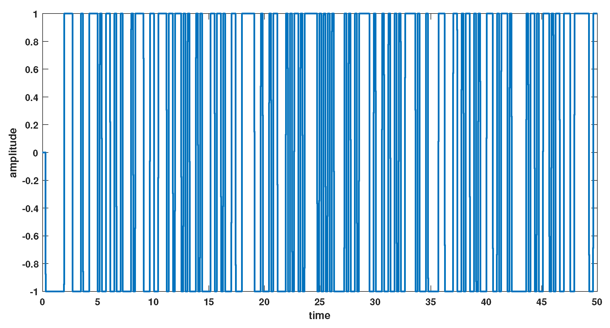
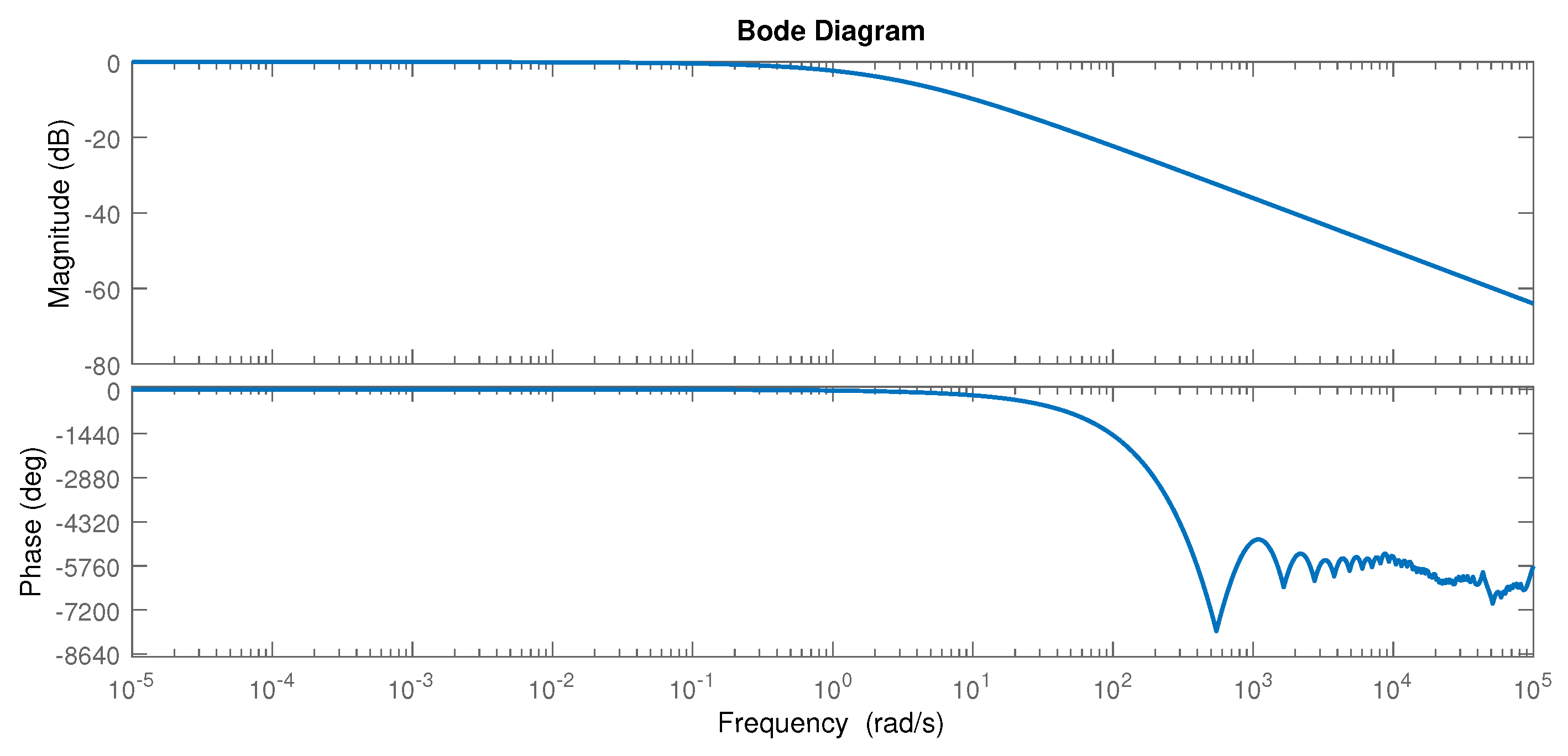
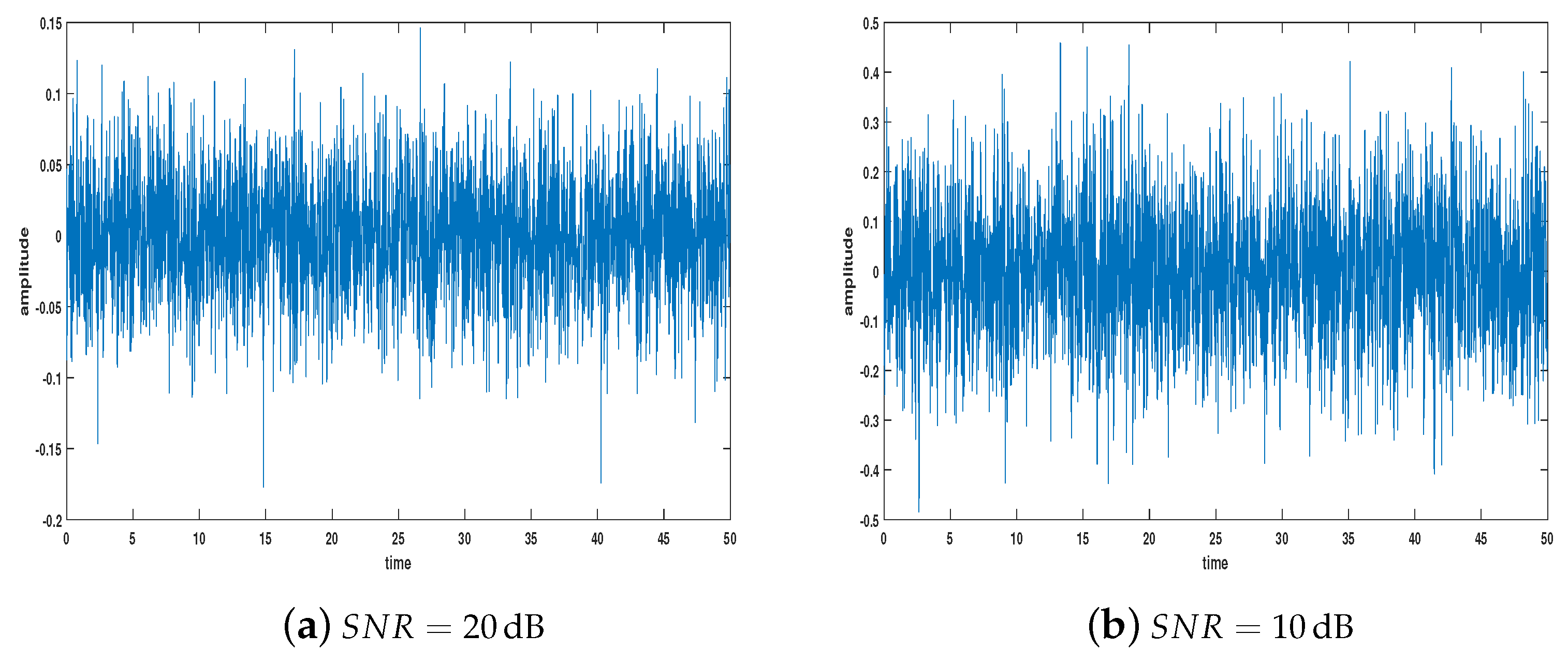
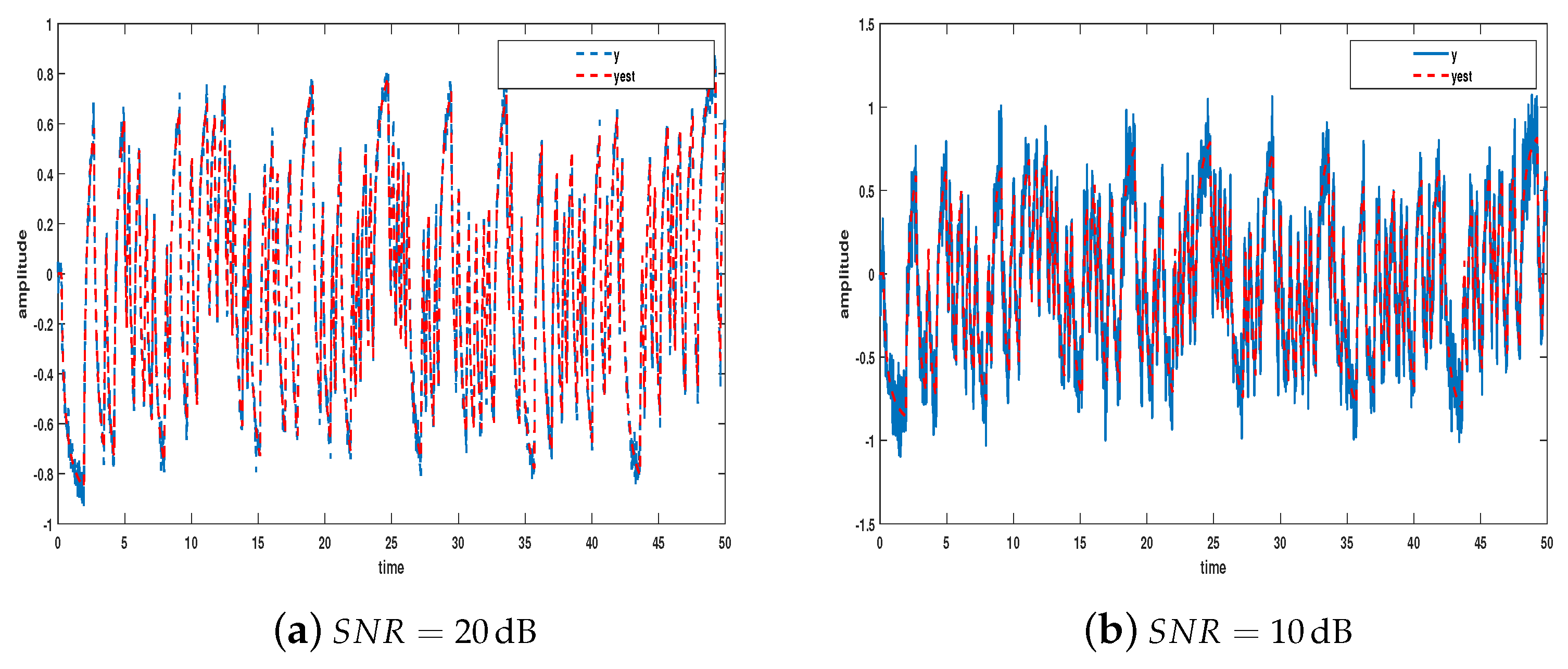
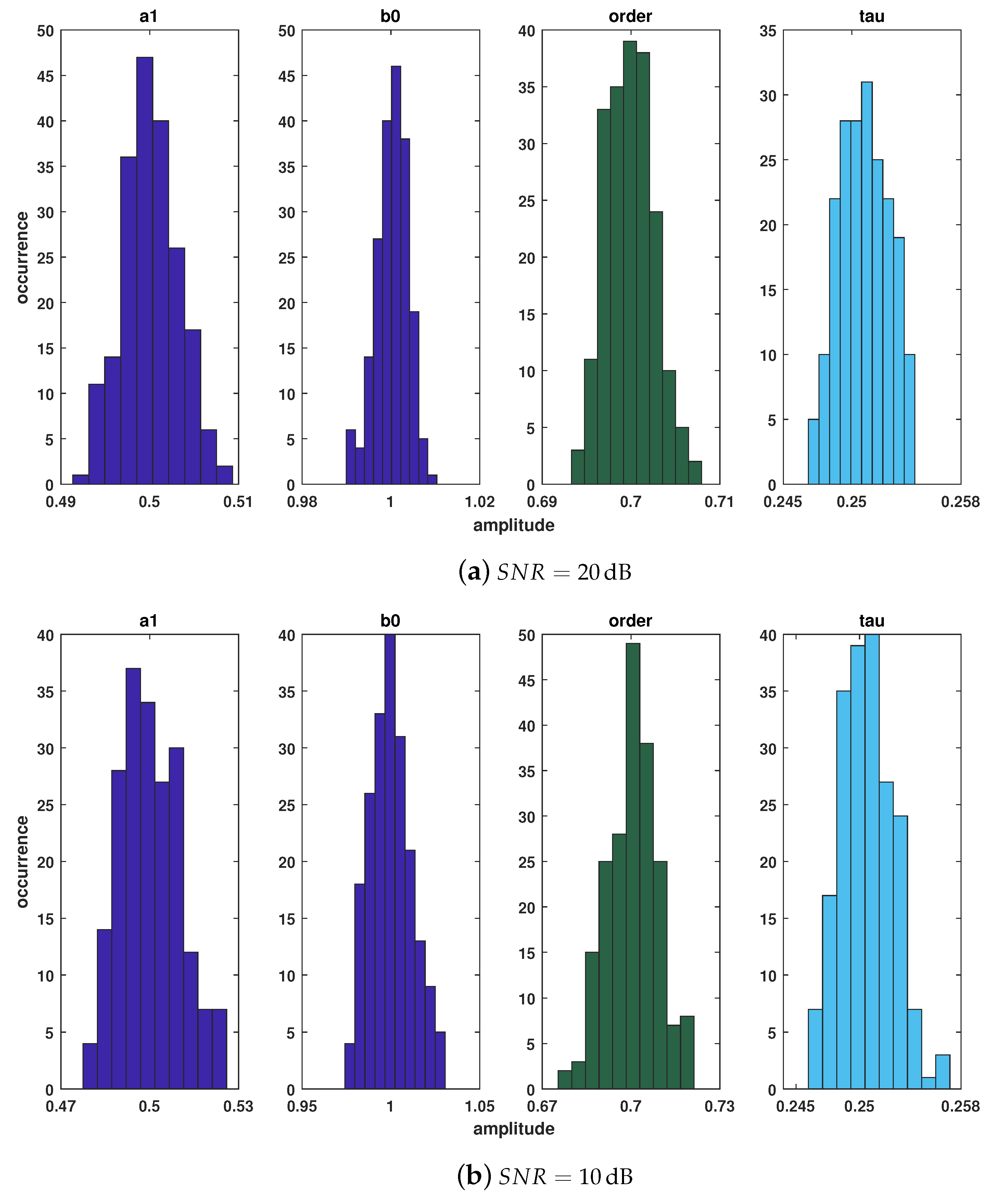
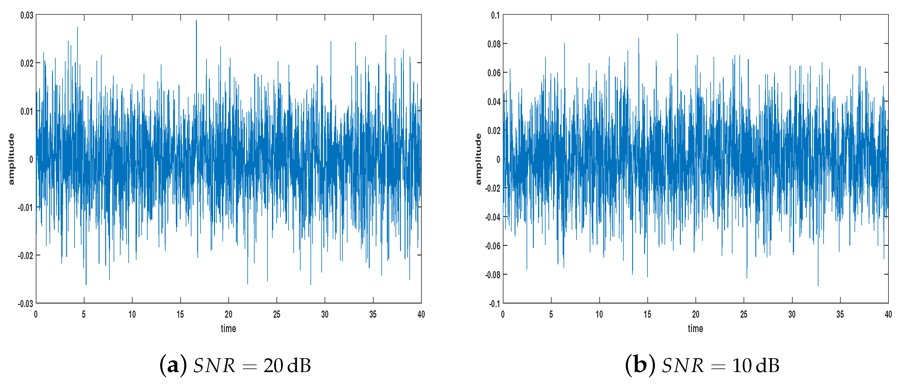
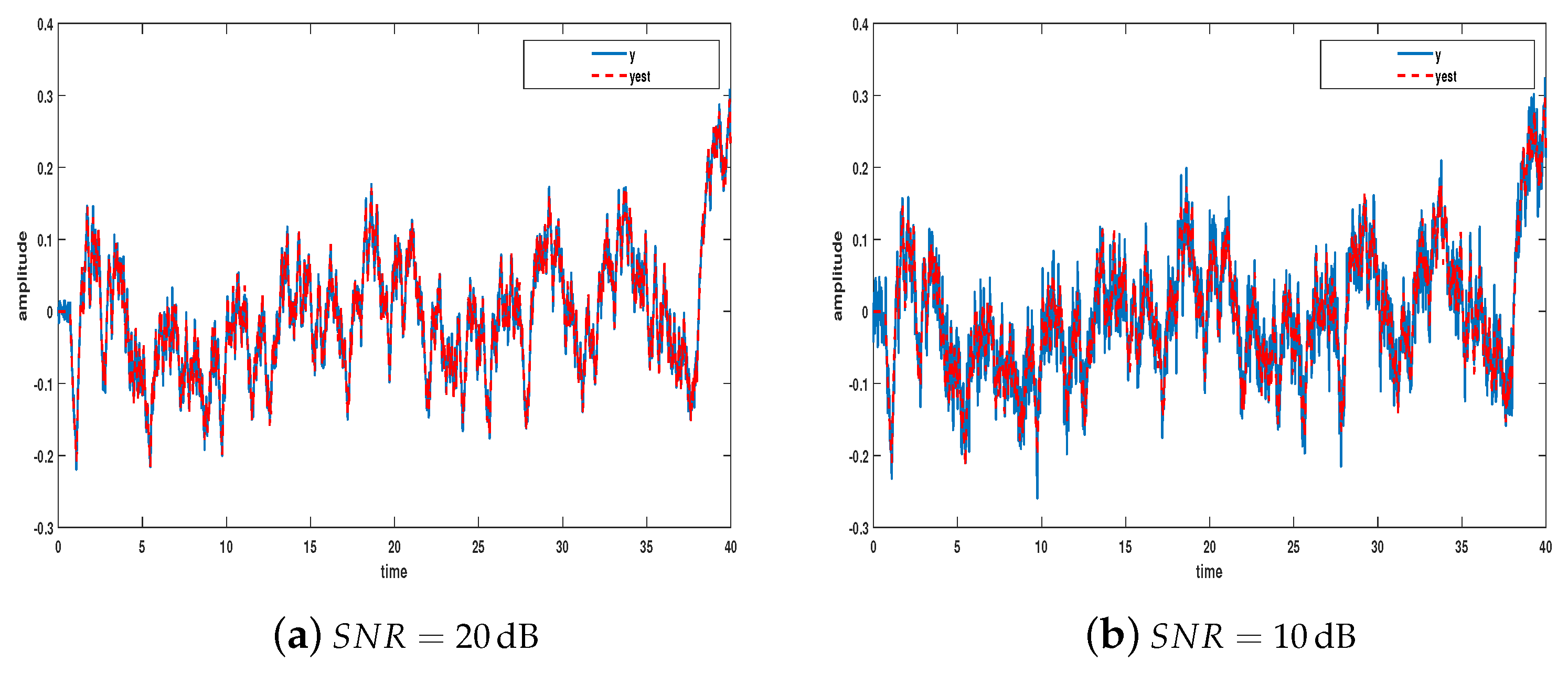
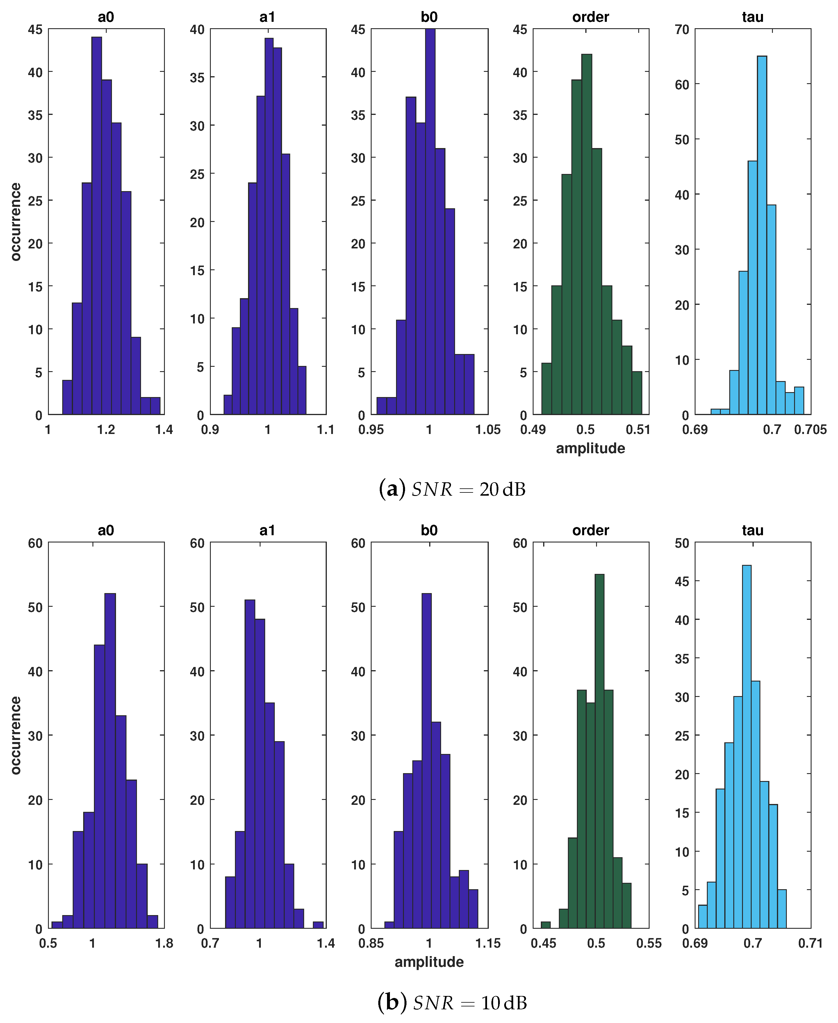
The purpose of this section is to demonstrate the performance of the developed identification approach through two numerical examples.

To evaluate the identification result, we define the mean squared error $\left(MSE\right)$ and the best fit rate $\left(BFR\right)$, respectively, as follows

$$MSE=\frac{1}{N_s}\sum _{k=1}^{N_s}\left(y\left(k\right)-\widehat{y}\left(k\right)\right),$$

(60)

where $\widehat{y}$ is the simulated response of the estimated model.

$$\mathrm{BFR}=\max \left\{1-\sqrt{\frac{{\displaystyle \sum _{\mathrm{k}=1}^{{\mathrm{N}}_{\mathrm{d}}}}{\left(\mathrm{y}\left({\mathrm{t}}_{\mathrm{k}}\right)-\widehat{\mathrm{y}}\left({\mathrm{t}}_{\mathrm{k}}\right)\right)}^2}{{\displaystyle \sum _{\mathrm{k}=1}^{{\mathrm{N}}_{\mathrm{d}}}}{\left(\mathrm{y}\left({\mathrm{t}}_{\mathrm{k}}\right)-\overline{\mathrm{y}}\right)}^2}},0\right\}.100\%,$$

(61)

where $\overline{y}$ is the mean of the output signal.

4.1. Example 1

Considering the following fractional order system with an unknown time-delay

$$y\left(t\right)=-a_1{D}^{\upsilon }y\left(t\right)+b_{0}u\left(t-\tau \right),$$

(62)

where the coefficients $a_1=0.50$, $b_0=1.00$, the fractional commensurate order $\upsilon =0.7$ and the time-delay $\tau =0.25$ s.

Figure 1 depicts the input signal $u\left(t\right)$ as a pseudo random binary sequence (PRBS) with uniform distribution between [−1 1]. This example’s sample period is set at $h=0.019$ s. $N_s=2631$ data points represents the sample size. The output observation-corrupting noise term $e\left(t\right)$ is a white Gaussian noise with a fixed signal-to-noise $\left(SN{R}_y\right)$ ratio, which is generated by

$$SN{R}_y=10\log \frac{{\displaystyle \sum _{k=1}^{Ns}}{\left(y-\overline{y}\right)}^2}{{\displaystyle \sum _{k=1}^{Ns}}{\left(e\left(k\right)\right)}^2}.$$

(63)

The parameters vector of the fractional model is given by

$$\rho =\left[\begin{array}{cccc}{a}_1& b_0& \upsilon & \tau \end{array}\right].$$

(64)

Figure 2 shows the Bode diagram of the system defined by (62).

The svf parameters are chosen respectively as: $\varpi =2$ rad/s and $\eta =1$.

The acquired findings are described in

Table 1. Mean and standard deviation of the fractional model parameter estimates obtained by the $FSTD$-$OE$ algorithm ($nmc=200$ runs, $SN{R}_y=20\mathrm{and}10$ [dB]): example 1.

		$\mathit{SNR}=20$ [dB]	$\mathit{SNR}=10$ [dB]
	$\mathit{True}$	$\widehat{\mathbf{\rho }}$	$\widehat{\mathbf{\rho }}$
$a_1$	$0.500$	$0.5001\pm 0.0031$	$0.501\pm 0.0101$
$b_0$	$1.000$	$1.0002\pm 0.0035$	$1.0008\pm 0.0118$
$\upsilon$	$0.700$	$0.6999\pm 0.0027$	$0.7009\pm 0.0086$
$\tau$	$0.250$	$0.2503\pm 0.0018$	$0.2508\pm 0.0021$

and

Table 2. $BFR$ and $MSE$ obtained by the $FSTD-OE$ algorithm ($nmc=200$ runs, $SN{R}_y=20$, $\mathrm{and}10$ [dB]): example 1.

	$\mathit{SNR}=20$ [dB]		$\mathit{SNR}=10$ [dB]
Method	$\mathit{MSE}$(%)	$\mathit{BFR}$ (%)	$\mathit{MSE}$ (%)	$\mathit{BFR}$ (%)
$FSTD-OE$	0.0429	99.00	0.16	98.85

, followed by a graphical representation in Figure 3, Figure 4 and Figure 5. It is evident from the values of the mean and standard deviation shown in Table 1 and the estimation error recapitulated in Table 2 that the $FOSTD-OE$ algorithm produces unbiased parameters estimates with low $MSE$ and standard deviation values. Therefore, the proposed algorithm gives accurate estimations in a noisy environment even if the value of the $SNR$ is low (10 [dB]).

The error between the true output $y\left(t\right)$ and $\widehat{y}\left(t\right)$ is plotted in Figure 3.

The true output $y\left(t\right)$ and the simulated output sequences $\widehat{y}\left(t\right)$ of the estimated models are plotted in Figure 4.

Figure 5 presents histograms that display the distribution of estimates and provide meaningful information. It is clear that these distributions are roughly symmetric and centered on the real values, which confirms the high accuracy of this approach.

This concludes that the proposed approach offers a good tradeoff in terms of consistency, variance, and estimation error.

4.2. Example 2

In this example, the input−output representation to be identified is given by the following equation

$$y\left(t\right)=-a_1{D}^{\upsilon }y\left(t\right)-a_2{D}^{2\upsilon }y\left(t\right)+b_{0}u\left(t-\tau \right),$$

(65)

where $a_1=1.2$, $a_2=1.00$, $b_0=1.00$, $\upsilon =0.5$ and $\tau =0.7$ s.

The input signal used in this example is depicted in Figure 6. The sampling period $h=0.0181$ s and $N_s=2209$ data.

The Bode diagram of the system defined by the Equation (65) is plotted in Figure 7.

The svf parameters are selected respectively as: $\varpi =1$ rad/s and $\eta =2$.

The parameter identification results are recorded in

Table 3. Mean and standard deviation of the fractional model parameter estimates obtained by the $FSTD$-$OE$ algorithm ($nmc=200$ runs, $SN{R}_y=20\mathrm{and}10$ [dB]): example 2.

	$\mathit{SNR}=20$ [dB]	$\mathit{SNR}=10$ [dB]
$a_1=1.200$	$1.1969\pm 0.0603$	$1.1849\pm 0.099$
$a_2=1.000$	$0.9997\pm 0.0271$	$1.0101\pm 0.0947$
$b_0=1.000$	$0.9990\pm 0.0153$	$0.9982\pm 0.0470$
$\upsilon =0.500$	$0.5001\pm 0.0038$	$0.4993\pm 0.0135$
$\tau =0.700$	$0.6992\pm 0.0018$	$0.6986\pm 0.0030$

and

Table 4. $BFR$ and $MSE$ obtained by the $FSTD-OE$ algorithm ($nmc=200$ runs, $SN{R}_y=20$$\mathrm{and}10$ [dB]): example 2.

	$\mathit{SNR}=20$ [dB]		$\mathit{SNR}=10$ [dB]
Method	$\mathit{MSE}$(%)	$\mathit{BFR}$ (%)	$\mathit{MSE}$ (%)	$\mathit{BFR}$ (%)
$FSTD-\mathrm{OE}$	0.340	98.92	0.540	96.02

which summarize the mean, standard deviation, $MSE$ and $BFR$ of the 200 Monte Carlo parameter estimations for fractional models. Despite the noise in the output, it can be seen from the identification results that the proposed method effectively estimates the system parameters

The error between the true output $y\left(t\right)$ and $\widehat{y}\left(t\right)$ is plotted in Figure 8.

The true output $y\left(t\right)$ and the simulated output sequences $\widehat{y}\left(t\right)$ of the estimated model are plotted for the two levels of noise in Figure 9.

It is clearly shown that the proposed method has a small identification error, and that the identification result is closer to the true one.

The statistical properties of the algorithm, plotted in Figure 10, are noticeable: the average values are very close to the real parameters, with very low standard deviations and $MSE$ and with $BFR$ approximately equal to one. Moreover, the distribution of the parameters is symmetric for the two levels of the $SNR$. The identification results confirm that the proposed method is able to identify the model coefficients, orders, and time delay.

The accuracy and precision of the suggested approach to detect both coefficients, fractional order differentiation, and time-delay in the situation of a noisy output signal and even with a large number of parameters (Case of example 2:5 parameters) are validated by simulation results based on two numerical cases. This indicates that the proposed method is suitable for the identification of fractional order time-delay systems.

5. Conclusions

This paper studies the identification of the fractional order system with time-delay. It is known that the obtained coefficient estimations of the fractional order differential equation using the least squares algorithm are biased. So, the bias correction procedure is applied in this work in order to compensate this introduced bias and to obtain accurate results. This procedure is combined with a nonlinear algorithm to identify iteratively the coefficients as well as the fractional order differentiation and the time-delay. The main features of the proposed method are: its consistency, its implementation simplicity, and its faster convergence. Two numerical examples were used to illustrate the validity of the proposed guidelines and technique.

In an effort to approach more realistic assumptions, it is planned to expand this work to the scenario when the input signal is influenced by additive noise.

References

1. Cois, O.; Oustaloup, A.; Poinot, T.; Battaglia, J. Fractional state variable filter for system identification by fractional model. In Proceedings of the European Control Conference (ECC), Porto, Portugal, 4–7 September 2001; pp. 2481–2486. [Google Scholar]
2. Peng, C.; Li, W.; Wang, Y. Frequency domain identification of fractional order time delay systems. In Proceedings of the 2010 Chinese Control and Decision Conference, Xuzhou, China, 26–28 May 2010; pp. 2635–2638. [Google Scholar]
3. Valério, D.; Sá da Costa, J. Identifying digital and fractional transfer functions from a frequency response. Int. J. Control 2011, 84, 445–457. [Google Scholar] [CrossRef]
4. Raïssi, T.; Aoun, M. On robust pseudo state estimation of fractional order systems. In Proceedings of the International Symposium on Positive Systems, Rome, Italy, 14–16 September 2016; pp. 97–111. [Google Scholar]
5. Yakoub, Z.; Naifar, O.; Amairi, M.; Chetoui, M.; Aoun, M.; Makhlouf, A.B. A Bias-Corrected Method for Fractional Linear Parameter Varying Systems. Math. Probl. Eng. 2022, 2022, 7278157. [Google Scholar] [CrossRef]
6. Naifar, O.; Ben Makhlouf, A. On the stabilization and observer design of polytopic perturbed linear fractional-order systems. Math. Probl. Eng. 2021, 2021, 6699756. [Google Scholar] [CrossRef]
7. Oustaloup, A.; Sabatier, J.; Lanusse, P.; Malti, R.; Melchior, P.; Moreau, X.; Moze, M. An overview of the CRONE approach in system analysis, modeling and identification, observation and control. IFAC Proc. Vol. 2008, 41, 14254–14265. [Google Scholar] [CrossRef] [Green Version]
8. Reyes-Melo, M.; Martinez-Vega, J.; Guerrero-Salazar, C.; Ortiz-Mendez, U. Modelling of relaxation phenomena in organic dielectric materials. Application of differential and integral operators of fractional order. J. Optoelectron. Adv. Mater. 2004, 6, 1037–1044. [Google Scholar]
9. Jallouli-Khlif, R.; Jelassi, K.; Melchior, P.; Trigeassou, J.C. Fractional modeling of rotor skin effect in induction machines. In Proceedings of the 4th IFAC Workshops on Fractional Differentiation and its Applications (IFAC FDA’10), Badajoz, Spain, 18–20 October 2010. [Google Scholar]
10. Jin, B.; Kian, Y. Recovery of the order of derivation for fractional diffusion equations in an unknown medium. SIAM J. Appl. Math. 2022, 82, 1045–1067. [Google Scholar] [CrossRef]
11. Krasnoschok, M.; Pereverzyev, S.; Siryk, S.V.; Vasylyeva, N. Regularized reconstruction of the order in semilinear subdiffusion with memory. In Proceedings of the International Conference on Inverse Problems, Shanghai, China, 12–14 October 2018; Springer: Singapore, 2018; pp. 205–236. [Google Scholar]
12. Krasnoschok, M.; Pereverzyev, S.; Siryk, S.V.; Vasylyeva, N. Determination of the fractional order in semilinear subdiffusion equations. Fract. Calc. Appl. Anal. 2020, 23, 694–722. [Google Scholar] [CrossRef]
13. Gu, W.; Wei, F.; Li, M. Parameter estimation for a type of fractional diffusion equation based on compact difference scheme. Symmetry 2022, 14, 560. [Google Scholar] [CrossRef]
14. Zaborovsky, V.; Meylanov, R. Informational network traffic model based on fractional calculus. In Proceedings of the 2001 International Conferences on Info-Tech and Info-Net. Proceedings (Cat. No. 01EX479), Beijing, China, 29 October–1 November 2001; Volume 1, pp. 58–63. [Google Scholar]
15. Ionescu, C.; Lopes, A.; Copot, D.; Machado, J.T.; Bates, J.H. The role of fractional calculus in modeling biological phenomena: A review. Commun. Nonlinear Sci. Numer. Simul. 2017, 51, 141–159. [Google Scholar] [CrossRef]
16. Dalir, M.; Bashour, M. Applications of fractional calculus. Appl. Math. Sci. 2010, 4, 1021–1032. [Google Scholar]
17. Sabatier, J.; Aoun, M.; Oustaloup, A.; Gregoire, G.; Ragot, F.; Roy, P. Fractional system identification for lead acid battery state of charge estimation. Signal Process. 2006, 86, 2645–2657. [Google Scholar] [CrossRef]
18. Victor, S.; Malti, R.; Garnier, H.; Oustaloup, A. Parameter and differentiation order estimation in fractional models. Automatica 2013, 49, 926–935. [Google Scholar] [CrossRef]
19. Battaglia, J.L.; Le Lay, L.; Batsale, J.C.; Oustaloup, A.; Cois, O. Utilisation de modèles d’identification non entiers pour la résolution de problèmes inverses en conduction. Int. J. Therm. Sci. 2000, 39, 374–389. [Google Scholar] [CrossRef]
20. Malti, R.; Victor, S.; Oustaloup, A.; Garnier, H. An optimal instrumental variable method for continuous-time fractional model identification. IFAC Proc. Vol. 2008, 41, 14379–14384. [Google Scholar] [CrossRef] [Green Version]
21. Wu, H.; Yuan, S.; Yin, C. A lithium-ion battery fractional order state space model and its time domain system identification. In Proceedings of the FISITA 2012 World Automotive Congress; Springer: Berlin/Heidelberg, Germany, 2013; pp. 795–805. [Google Scholar]
22. Yakoub, Z.; Amairi, M.; Chetoui, M.; Aoun, M. On the Closed-Loop System Identification with Fractional Models. Circuits Syst. Signal Process. 2015, 34, 3833–3860. [Google Scholar] [CrossRef]
23. Mani, A.K.; Narayanan, M.; Sen, M. Parametric identification of fractional-order nonlinear systems. Nonlinear Dyn. 2018, 93, 945–960. [Google Scholar] [CrossRef]
24. Zhang, B.; Tang, Y.; Zhang, J.; Lu, Y. Coefficients and Orders Identification of Fractional Order Systems Based on Block Pulse Functions Through Two-Stage Algorithm. J. Dyn. Syst. Meas. Control 2022, 144, 071001. [Google Scholar] [CrossRef]
25. Narang, A.; Shah, S.L.; Chen, T. Continuous-time model identification of fractional-order models with time delays. IET Control Theory Appl. 2011, 5, 900–912. [Google Scholar] [CrossRef] [Green Version]
26. Wang, L.; Cheng, P.; Wang, Y. Frequency domain subspace identification of commensurate fractional order input time delay systems. Int. J. Control Autom. Syst. 2011, 9, 310–316. [Google Scholar] [CrossRef]
27. Liao, Z.; Peng, C.; Wang, Y. A frequency-domain identification algorithm for MIMO fractional order systems with time-delay in state. In Advanced Materials Research; Trans Tech Publications Ltd.: Stafa-Zurich, Switzerland, 2012; Volume 383, pp. 4397–4404. [Google Scholar]
28. Zhuting, Z.; Zeng, L.; Shu, L.; Cheng, P.; Yong, W. Subspace-based identification for fractional order time delay systems. In Proceedings of the 31st Chinese Control Conference, Hefei, China, 25–27 July 2012; pp. 2019–2023. [Google Scholar]
29. Ahmed, S. Parameter and delay estimation of fractional order models from step response. IFAC-PapersOnLine 2015, 48, 942–947. [Google Scholar] [CrossRef]
30. Tang, Y.; Li, N.; Liu, M.; Lu, Y.; Wang, W. Identification of fractional-order systems with time delays using block pulse functions. Mech. Syst. Signal Process. 2017, 91, 382–394. [Google Scholar] [CrossRef]
31. Gao, Z.; Lin, X.; Zheng, Y. System identification with measurement noise compensation based on polynomial modulating function for fractional-order systems with a known time-delay. ISA Trans. 2018, 79, 62–72. [Google Scholar] [CrossRef] [PubMed]
32. Moghaddam, M.J.; Mojallali, H.; Teshnehlab, M. Recursive identification of multiple-input single-output fractional-order Hammerstein model with time delay. Appl. Soft Comput. 2018, 70, 486–500. [Google Scholar] [CrossRef]
33. Kothari, K.; Mehta, U.; Vanualailai, J. A novel approach of fractional-order time delay system modeling based on Haar wavelet. ISA Trans. 2018, 80, 371–380. [Google Scholar] [CrossRef]
34. Alagoz, B.B.; Tepljakov, A.; Ates, A.; Petlenkov, E.; Yeroglu, C. Time-domain identification of one noninteger order plus time delay models from step response measurements. Int. J. Model. Simul. Sci. Comput. 2019, 10, 1941011. [Google Scholar] [CrossRef]
35. Hashemniya, F.; Tavakoli-Kakhki, M.; Azarmi, R. Coefficients and Delay Estimation of the General Form of Fractional Order Systems Using Non-Ideal Step Inputs. IFAC-PapersOnLine 2020, 53, 590–597. [Google Scholar] [CrossRef]
36. Sin, M.H.; Sin, C.; Ji, S.; Kim, S.Y.; Kang, Y.H. Identification of fractional-order systems with both nonzero initial conditions and unknown time delays based on block pulse functions. Mech. Syst. Signal Process. 2022, 169, 108646. [Google Scholar] [CrossRef]
37. Yakoub, Z.; Chetoui, M.; Amairi, M.; Aoun, M. A bias correction method for fractional closed-loop system identification. J. Process Control 2015, 33, 25–36. [Google Scholar] [CrossRef]
38. Lu, Y.; Tang, Y.; Zhang, X.; Wang, S. Parameter identification of fractional order systems with nonzero initial conditions based on block pulse functions. Measurement 2020, 158, 107684. [Google Scholar] [CrossRef]
39. Li, C.; Qian, D.; Chen, Y. On Riemann-Liouville and Caputo derivatives. Discret. Dyn. Nat. Soc. 2011, 2011, 562494. [Google Scholar] [CrossRef] [Green Version]
40. Malti, R.; Aoun, M.; Sabatier, J.; Oustaloup, A. Tutorial on system identification using fractional differentiation models. In Proceedings of the 14th IFAC Symposium on System Identification, Newcastle, Australia, 29–31 March 2006; pp. 606–611. [Google Scholar]
41. Ivanov, D.V.; Sandler, I.L.; Kozlov, E.V. Identification of fractional linear dynamical systems with autocorrelated errors in variables by generalized instrumental variables. IFAC-PapersOnLine 2018, 51, 580–584. [Google Scholar] [CrossRef]
42. Ljung, L. System Identification—Theory for the User, 2nd ed.; PrenticeHall: Upper Saddle River, NJ, USA, 1999; Volume 101. [Google Scholar]
Figure 1. The excitation signal.
Mathematics 10 03028 g001
Figure 2. The bode diagrams of the system (62).
Mathematics 10 03028 g002
Figure 3. The output error of example 1.
Mathematics 10 03028 g003
Figure 4. The true and the estimated output signals of example 1.
Mathematics 10 03028 g004
Figure 5. The histograms of the process estimates of example 1 with the F O S T D - O E algorithm S N R y = 20 and 10 [ dB ] n m c = 200 runs.
Mathematics 10 03028 g005
Figure 6. The excitation signal of the system (65).
Mathematics 10 03028 g006
Figure 7. The bode diagrams of the system (65).
Mathematics 10 03028 g007
Figure 8. The output error of example 2.
Mathematics 10 03028 g008
Figure 9. The true and the estimated output signals of example 2.
Mathematics 10 03028 g009
Figure 10. The histograms of the process estimates of example 2 with the F S T D - O E algorithm S N R y = 20 [ dB ] n m c = 200 runs.
Mathematics 10 03028 g010