The Existence and Uniqueness of Riccati Fractional Differential Equation Solution and Its Approximation Applied to an Economic Growth Model

Abstract

This work proposes and investigates the existence and uniqueness of solutions of Riccati Fractional Differential Equation (RFDE) with constant coefficients using Banach’s fixed point theorem. This theorem is the uniqueness theorem of a fixed point on a contraction mapping of a norm space. Furthermore, the combined theorem of the Adomian Decomposition Method (ADM) and Kamal’s Integral Transform (KIT) is used to convert the solution of the Fractional Differential Equation (FDE) into an infinite polynomial series. In addition, the terms of an infinite polynomial series can be decomposed using ADM, which assumes that a function can be decomposed into an infinite polynomial series and nonlinear operators can be decomposed into an Adomian polynomial series. The final result of this study is to find a solution of the RFDE approach to the economic growth model with a quadratic cost function using the combined ADM and KIT. The results showed that the RFDE solution on the economic growth model using the combined ADM and KIT showed a very good performance. Furthermore, the numerical solution of RFDE on the economic growth model is presented at the end of this work.

1. Introduction

Fractional calculus has played a significant role in the economics growth model [1,2], financial risks [3,4], the effects of market confidence [5], digital imaging of bank slips [6], supply chain financial systems [7], bank data [8], stock markets [9], image encryption [10,11], robotics [12], Field-Programmable Analog Array [13], Field-Programmable Gate Array [14], and random bits generators [15].

The Adomian decomposition method (ADM) is a powerful technique for solving linear and nonlinear functional equations. In addition, the ADM method has been widely combined with other methods to solve practical applications. Wazwaz [16] proposed a combined form of the Laplace transform method with the Adomian decomposition method to analyze the nonlinear Volterra integro–differential equations. Babolian et al. [17] investigated a combination of the Adomian decomposition method (ADM) and the spectral Adomian decomposition method (SADM) for nonlinear fractional differential equations. Varsoliwala and Singh [18] presented a combination of the Adomian decomposition method (ADM) and the Elzaki Transform methods (ETM) for water infiltration in unsaturated soils. Ahmed and Elzaki [19] studied the combination of Sumudu transforms and the Adomian decomposition method to solve nonlinear Volterra Integro-Differential equations. Chindhe and Kiwne [20] introduced the combined natural transform and Adomian decomposition method to solve the nonlinear voltrra integro-differential equations of the first and second types. Johansyah et al. [21] described the combined method between the Adomian decomposition method and the Kamal integral transformation for solving differential equations of fractional order. Ramezani et al. [22] proposed combining the Adomian decomposition method with Fourier transformation to solve the squeezing flow influenced by a magnetic field. Liaqat et al. [23] analyzed the combination of the combined Shehu transform (CST) and the Adomian decomposition method (ADM) to obtain the approximate and exact analytical solutions to linear-nonlinear fractional partial differential equations. Khandelwal and Khandelwal [24] studied the combination between the Adomian decomposition method and Mohand transform for handling a differential equation of mixing layer that arises in a viscous incompressible fluid. Johansyah et al. [2] presented the combined theorem between Adomian Polynomial Decomposition and Kashuri–Fundo Transformation methods to solve the economic growth acceleration model with memory effects. However, the combination between the Adomian Decomposition Method (ADM) and Kamal’s Integral Transform needs further development, especially to complete the economic growth model.

In mathematics, various scientists have studied the uniqueness theorem intensively [25,26,27,28]. Diethelm and Ford [25] proved the existence and uniqueness of nonlinear fractional differential equations using the Fixed-Point Theorem of Banach Space. Furthermore, Lakshmikantham and Vatsala [26] investigated the basic theory for the initial value problem of fractional differential equations involving Riemann–Liouville employing the classical approach. In addition, they have considered the theory of inequalities, local existence, extremal solutions, comparison results, and global existence of solutions. Benlabes et al. [27] investigated the existence and uniqueness of the initial value problem of nonlinear fractional differential equations. They found a single solution of nonlinear fractional differential equations using the help of contraction mapping and Banach’s contraction principle. In addition, using Schaefer’s fixed-point theorem, T has at least a fixed point on C([0, 1], R). Elsaid et al. [28] proved the existence and uniqueness of RFDE with variable coefficients and the definition of Caputo fractional derivatives with the help of Lipschitz conditions and continuous set collections. However, the research above cannot explain the existence and uniqueness of the non-linear RFDE with constant coefficients in the economic growth model. In more detail, references related to fractional order can be seen at [29,30,31,32].

This study’s main contribution and novelty are investigating the existence and uniqueness of the non-linear RFDE with constant coefficients in the economic growth model. Furthermore, to find out the non-linear RFDE approach solution on the economic growth model for the order $0<\alpha \le 1$.

The structure of this paper is as follows: Section 2 provides background notions related to the modification and development of the theorem of existence and uniqueness RFDE with constant coefficients and combining ADM with Kamal Integral Transform. In Section 3, the main results about the existence and uniqueness theorem of RFDE solutions and the theorem for finding solutions to the RFDE approach using the ADM Theorem and Kamal Integral Transformation. Section 4 presents our conclusions.

2. Preliminaries

This section presents the basic theories and theorems related to modifying and developing the theorem of existence and uniqueness of RFDE with constant coefficients. It combines ADM with Kamal’s Integral Transform as follows:

Theorem 1.

Given the Riccati Fractional Differential Equation.

$$D_t^{\alpha }y\left(t\right)=a+by\left(t\right)+c{y}^2\left(t\right), t>0, 0<\alpha <1$$

(1)

where the initial value of$y\left(0\right)=y_0$and$a,b,c$is a constant coefficient. Let$a+by\left(t\right)+c{y}^2\left(t\right)$be continuous for every t > 0, then the solution of Equation (1) is equivalent to the solution of the integral Equation (2), that is

$$y\left(t\right)=y_0+I^{\alpha }\left(a+by\left(t\right)+c{y}^2\left(t\right)\right).$$

(2)

Proof. 

Suppose that the interval $A=\left[0,n\right]$ with $n<\infty$ and $C\left(A\right)$ is the set of all continuous functions defined on A with the norm $\Vert y\Vert =\underset{t\in A }{\sup }\left|y\left(t\right)\right|$.

Step 1: It will be proved that if y(t) satisfies the solution of Equation (1), then y(t) satisfies Equation (2).

Caputo’s fractional integral operator is of the form:

$$D_t^{\alpha }y\left(t\right)=I^{n-\alpha }{D}_t^{n}y\left(t\right),$$

If n = 1 i.e., $D_t^{\alpha }y\left(t\right)=I^{1-\alpha }{D}_t^{1}y\left(t\right)$, then Equation (1) can be written as follows:

$$I^{\left(1-\alpha \right)}{D}_t^{1}y\left(t\right)=a+by\left(t\right)+c{y}^2\left(t\right), t>0, 0<\alpha <1.$$

(3)

Furthermore, if both sides of Equation (3) are operated using the operator $I^{\alpha },$ then the integral equation is obtained as follows:

$$\begin{array}{ccc}\hfill I^{\alpha }\left[I^{\left(1-\alpha \right)}dy\left(t\right)\right]& =& I^{\alpha }\left[a+by\left(t\right)+c{y}^2\left(t\right)\right],\hfill \\ \hfill & & \hfill \\ \hfill I^{1}dy\left(t\right)& =& I^{\alpha }\left[a+by\left(t\right)+c{y}^2\left(t\right)\right],\hfill \\ \hfill {{\displaystyle \int }}_0^{t}dy\left(t\right)& =& I^{\alpha }\left[a+by\left(t\right)+c{y}^2\left(t\right)\right],\hfill \\ \hfill {y\left(t\right)|}_0^t& =& I^{\alpha }\left[a+by\left(t\right)+c{y}^2\left(t\right)\right],\hfill \\ \hfill y\left(t\right)-y\left(0\right)& =& I^{\alpha }\left[a+by\left(t\right)+c{y}^2\left(t\right)\right],\hfill \\ \hfill y\left(t\right)-y_0& =& I^{\alpha }\left[a+by\left(t\right)+c{y}^2\left(t\right)\right],\hfill \\ \hfill & & y\left(t\right)=y_0+I^{\alpha }\left[a+by\left(t\right)+c{y}^2\left(t\right)\right].\hfill \end{array}$$

It is proved that if y(t) satisfies the solution of Equation (1), then y(t) satisfies Equation (2).

Before proving that Equation (2) is a solution to Equation (1), we will first show that $I^{\alpha }{\left[a+by\left(t\right)+c{y}^2\left(t\right)\right]}_{t=0}=0.$

If t = 0, then Equation (2) becomes:

$$\begin{array}{cc}y\left(t\right)=& y_0+I^{\alpha }\left(a+by\left(t\right)+c{y}^2\left(t\right)\right),\hfill \\ & y\left(0\right)=y_0+I^{\alpha }{\left[a+by\left(t\right)+c{y}^2\left(t\right)\right]}_{t=0}.\hfill \end{array}$$

While it is known that the initial value requirement is y(0) = y₀, then:

$$y_0=y_0+I^{\alpha }{\left[a+by\left(t\right)+c{y}^2\left(t\right)\right]}_{t=0} ,$$

So that obtained:

$$I^{\alpha }{\left[a+by\left(t\right)+c{y}^2\left(t\right)\right]}_{t=0}=0.$$

(4)

Step 2: It will be proved if y(t) satisfies Equation (2), then y(t) satisfies the solution of Equation (1).

If Equation (2) is derived with respect to t, then we obtain:

$$\begin{array}{c}\hfill \frac{dy\left(t\right)}{dt}=\frac{d{y}_0}{dt}+\frac{d}{dt}{I}^{\alpha }\left[a+by\left(t\right)+c{y}^2\left(t\right)\right],\hfill \\ \hfill \frac{dy\left(t\right)}{dt}=0+\frac{d}{dt}{I}^{\alpha }\left[a+by\left(t\right)+c{y}^2\left(t\right)\right].\hfill \end{array}$$

If both sides are operated with operator $I^{1-\alpha }$, then we obtain [33]:

$$\begin{array}{c}{I}^{1-\alpha }\frac{dy\left(t\right)}{dt}=I^{1-\alpha }\frac{d}{dt}{I}^{\alpha }\left[a+by\left(t\right)+c{y}^2\left(t\right)\right],\\ I^{1-\alpha }\frac{dy\left(t\right)}{dt}=\frac{d}{dt}{I}^{1-\alpha }{I}^{\alpha }\left[a+by\left(t\right)+c{y}^2\left(t\right)\right],\\ I^{1-\alpha }\frac{dy\left(t\right)}{dt}=\frac{d}{dt}{I}^{1-\alpha +\alpha }\left[a+by\left(t\right)+c{y}^2\left(t\right)\right],\\ I^{1-\alpha }\frac{dy\left(t\right)}{dt}=\frac{d}{dt}I\left[a+by\left(t\right)+c{y}^2\left(t\right)\right],\\ I^{1-\alpha }{I}^{-1}y\left(t\right)=I^{-1}I\left[a+by\left(t\right)+c{y}^2\left(t\right)\right],\\ I^{1-\alpha }{I}^{-1}y\left(t\right)=I^{-1+1}\left[a+by\left(t\right)+c{y}^2\left(t\right)\right],\\ I^{-\alpha }y\left(t\right)=\left[a+by\left(t\right)+c{y}^2\left(t\right)\right],\\ D_t^{\alpha }y\left(t\right)=a+by\left(t\right)+c{y}^2\left(t\right).\end{array}$$

(5)

If t = 0, then Equation (2) becomes:

$$\begin{array}{c}y\left(0\right)=y\left(0\right)+I^{\alpha }{\left[a+by\left(t\right)+c{y}^2\left(t\right)\right]}_{t=0}\\ \left(2\right)y\left(0\right)=y\left(0\right)+I^{\alpha }{\left[a+by\left(t\right)+c{y}^2\left(t\right)\right]}_{t=0}\end{array}$$

Based on Equation (4), the initial value is obtained as follows:

$$y\left(0\right)=y_0 .$$

(6)

Thus, from Equations (5) and (6), it can be concluded that if y(t) satisfies Equation (2), then y(t) satisfies the solution to Equation (1).

Thus, it is proved that the solution of the Riccati Fractional Differential Equation (1) is equivalent to the integral Equation (2). □

Lemma 1.

Let$f\left(t,y\left(t\right)\right)=a+by\left(t\right)+c{y}^2\left(t\right)$, where$f\left(t,y\right):\left[0,n\right]\times ℝ\to ℝ$, a, b, c are real constants and y(t) is a continuous function that is finite in M, so that the function$f\left(t,y\left(t\right)\right)$satisfies Lipschitz’s condition for the variable y, namely |$f\left(t,y_1\left(t\right)\right)-f\left(t,y_2\left(t\right)\right)$|$\le$K |$y_1\left(t\right)-y_2\left(t\right)|$with Lipschitz constant$K=K_1+K_{2}M.$

Proof. 

Let $f\left(t,y\left(t\right)\right)=a+by\left(t\right)+c{y}^2\left(t\right)$, where $f\left(t,y\right):\left[0,n\right]\times ℝ\to ℝ$ and take any y(t) finite continuous function in M, then $f\left(t,y\left(t\right)\right)$ is derived with respect to y obtained:

$$\left|\frac{\partial f}{\partial y}\right|=\left|b+2cy\left(t\right)\right|\le \left|b\right|+\left|2cy\left(t\right)\right|=\left|b\right|+2\left|c\right|\left|y\left(t\right)\right|\le K_1+K_{2}M=K.$$

(7)

Therefore, the function $f\left(t,y\left(t\right)\right)$ satisfies the Lipschitz condition for the variable y, with the Lipschitz constant $K=K_1+K_{2}M$, since the derivative of the function is bounded. □

Furthermore, this section presents the theory and basic concepts of RFDE solutions using the Combined Theorem of the Adomian Decomposition Method with Kamal Integral Transformation.

Theorem 2.

Cauchy Criteria [34].

The sequence of real functions$\left(f_n\right)$converges uniformly to f on A if and only if for every$\epsilon >0$there are a number$N\in \mathbb{N}$such that for every$n,m\in \mathbb{N}$with$n,m\ge N$and every$x\in A$obtained:

$$\left|f_n\left(x\right)-f_m\left(x\right)\right|<\epsilon .$$

Theorem 3 ([34]).

 

Given$\left(f_n\right)$the sequence of continuous functions on$A\subset ℝ$. If$f_n$converges uniformly to f at A, then f is continuous at A.

Theorem 4.

If$C\left(A\right)=\left\{f:A\to ℝ | is continuous at A=\left[0,n\right]\right\}$with norm$\Vert f\Vert =\underset{x\in A}{\mathit{sup}}\left|f\left(x\right)\right|$. Then C(A) is a complete normed space (Banach space).

Proof. 

It is known that C(A) is a normed space with the norm $\Vert f\Vert =\underset{x\in A}{\mathit{sup}}\left|f\left(x\right)\right|$, then we will prove that C(A) is complete.

Take ($f_n)$ the Cauchy sequence in the normed space C(A), meaning that for every $\epsilon >0$ there are $N\in \mathbb{N}$, so for every $m,n\ge N$ obtained:

$$\Vert f_n-f_m\Vert =\underset{x\in A}{\sup }\left|f_n\left(x\right)-f_m\left(x\right)\right|<\epsilon$$

for every x ∈ A applies $\left|f_n\left(x\right)-f_m\left(x\right)\right|<\epsilon$, for every m, n ≥ N.

Thus, the sequence of real numbers ($f_n\left(x\right)$) is a Cauchy sequence in $ℝ.$ Since $ℝ$ is complete it means that there is a real function $f:A\to ℝ$ such that the sequence of real numbers ($f_n\left(x\right))$ converges to $f\left(x\right)\in ℝ$ for every x.

Furthermore, we will prove that the function f is continuous on A.

Based on Theorem 2, namely the Cauchy Criteria Theorem, if the sequence of real numbers $\left(f_n\left(x\right)\right)$ satisfies $\left|f_n\left(x\right)-f_m\left(x\right)\right|<\epsilon$, for every x ∈ A and m, n ≥ N, then f_n converges uniformly to f, so that the Cauchy sequence $f_n$ converges to f. Since the sequence of functions, $f_n$, converges uniformly to function f and the function $f_n$ for every n ∈ N is continuous on A, so according to Theorem 3, the function f is also continuous on A or f ∈ C(A). Thus, it can be concluded that the Cauchy sequence ($f_n$) converges to f ∈ C(A).

So, C(A) is a normed space completed or C(A) is a Banach space. □

Definition 1.

Given a set of functions:

$$S=\left\{f\left(x\right):\exists M,k_1,k_2>0,\left|f\left(x\right)\right|<M{e}^{\frac{\left|x\right|}{k_j}},x\in {\left(-1\right)}^j\times \left[0,\infty \right)\right\}$$

Kamal’s transformation is defined as:

$$\mathcal{G}\left[f\left(x\right)\right]=G\left(v\right)=\underset{0}{\overset{\infty }{{\displaystyle \int }}}f\left(x\right)e^{-\frac{x}{v}}dx,x\ge 0,k_1\le v\le k_2.$$

Furthermore, the inverse of the Kamal transformation is denoted by:

$${\mathcal{G}}^{-1}\left[G\left(v\right)\right]=f\left(x\right), x\ge 0.$$

The following are some cases of Kamal transformations for the following simple functions:

f(x) = 1 where x≥ 0, based on Definition 1, we obtain:

$$\begin{array}{c}\mathcal{G}\left[f\left(x\right)\right]=G\left(v\right)=\underset{0}{\overset{\infty }{{\displaystyle \int }}}f\left(x\right)e^{-\frac{x}{v}}dx,x\ge 0,k_1\le v\le k_2.\\ \mathcal{G}\left[1\right]=G\left(v\right)=\underset{0}{\overset{\infty }{{\displaystyle \int }}}{e}^{-\frac{x}{v}}dx={\left[-v{e}^{-\frac{x}{v}}\right]}_0^{\infty }=v. \end{array}$$

f (x) = x, where x≥ 0, based on Definition 1 and using partial integrals, we obtain:

$$\begin{array}{c}\mathcal{G}\left[f\left(x\right)\right]=G\left(v\right)=\underset{0}{\overset{\infty }{{\displaystyle \int }}}f\left(x\right)e^{-\frac{x}{v}}dx,x\ge 0,k_1\le v\le k_2.\\ \mathcal{G}\left[x\right]=G\left(v\right)=\underset{0}{\overset{\infty }{{\displaystyle \int }}}x{e}^{-\frac{x}{v}}dx=v^2. \end{array}$$

Such that, for$f\left(x\right)=x^n$where x≥ 0, we obtain:

$$\mathcal{G}\left[x^n\right]=n!v^{n+1}.$$

Based on that, for$n=\alpha$, dengan$\alpha$is a fractional number, then obtained:

$$\mathcal{G}\left[x^{\alpha }\right]=\mathsf{\Gamma }\left(\alpha +1\right)v^{\alpha +1}.$$

(8)

Definition 2 ([35]).

The Caputo fractional derivative of the function f with respect to x of the order$\alpha$, where$\alpha >0$, is defined as:

$${}_a{}^{C}D_x^{\alpha }f\left(x\right)=\frac{1}{\mathsf{\Gamma }\left(n-\alpha \right)}\underset{a}{\overset{x}{{\displaystyle \int }}}{\left(x-u\right)}^{n-\alpha -1}{f}^{\left(n\right)}\left(u\right)du,n-1<\alpha \le n$$

Theorem 5 ([36]).

Let G(v) be the Kamal transformation of f(x), then:

• $\mathcal{G}\left[f^{\prime }\left(x\right)\right]=\frac{1}{v}G\left(v\right)-f\left(0\right)$,
• $\mathcal{G}\left[f^{″}\left(x\right)\right]=\frac{1}{v^2}G\left(v\right)-\frac{1}{v}f\left(0\right)-f^{\prime }\left(0\right)$,
• $\mathcal{G}\left[f^{\left(n\right)}\left(x\right)\right]=\frac{1}{v^n}G\left(v\right)-\sum _{k=0}^{n-1}\frac{f^{\left(k\right)}\left(0\right)}{v^{n-k-1}}$.

Theorem 6 ((Kamal Transformation Theorem) [36]).

 

The Kamal transformation of the Caputo fractional derivative for$a=0$is defined as:

$$\mathcal{G}\left[{}_{ }{}^{C}D_x^{\alpha }f\left(x\right)\right]=\frac{G\left(v\right)}{v^{\alpha }}-{\displaystyle \sum }_{k=0}^{n-1}\frac{f^{\left(k\right)}\left(0\right)}{v^{\alpha -k-1}},n-1<\alpha \le n.$$

The inverse of the Kamal transformation is denoted by${\mathcal{G}}^{-1}\left[G\left(v\right)\right]=f\left(x\right)$,$x\ge 0$.

For$\alpha$fractional number, then:

$$\mathcal{G}\left[x^{\alpha }\right]=\mathsf{\Gamma }\left(\alpha +1\right)v^{\alpha +1}.$$

Thus, for$\alpha$fractional numbers, the Inverse of the Kamal Integral Transform is:

$${\mathcal{G}}^{-1}\left[v^{\alpha +1}\right]=\frac{x^{\alpha }}{\Gamma \left(\alpha +1\right)}.$$

(9)

2.1. Banach Fixed Point Theorem

As it was stated and proved in the class notes, we have that in a complete metric space a contraction must map a point to itself; that is, it must have a fixed point, and even more, it is unique.

Theorem 7 (Banach’s Fixed Point Theorem).

 

Let X be a complete metric space and f be a contraction on X. Then there exists a unique x* such that f (x*) = x*.

Definition 3 (Contraction).

 

Let X be a metric space, and f: X. We will say that f is a contraction if there exists some 0 < k < 1, such that d (f(x), f(x*)) ≤ kd (x, y) for all x, y ϵ X. The inf of such k’s is called the contraction coefficient.

The Banach Fixed Point Theorem is also called the contraction mapping theorem, and it is in general use to prove that a unique solution to a given equation exists.

2.2. Adomian Decomposition Method

Given a fractional order differential equation as follows [37]:

$$D_t^{\alpha }y\left(t\right)+Ny\left(t\right)+Ry\left(t\right)=g\left(t\right) \mathrm{and} \mathrm{the} \mathrm{initial} \mathrm{condition} \mathrm{is} y\left(0\right)=c$$

(10)

where $D_t^{\alpha }\equiv {}^{C}D_t^{\alpha }$ is the Caputo fractional derivative operator with $0<\alpha \le 1$, N is the nonlinear operator, R is the linear operator, g is the function that shows the nonhomogeneity of the differential equation, and y is the function to be determined. Equation (10) can be rewritten with $D_t^{\alpha }y\left(t\right)$ as the subject:

$$D_t^{\alpha }y\left(t\right)=g\left(t\right)-Ny\left(t\right)-Ry\left(t\right)$$

(11)

Since $D_t^{\alpha }$ is a fractional derivative operator, the inverse is a fractional integral operator $I^{\alpha }=D_t^{-\alpha }$, such that when both sides of Equation (11) are integrated by I^α, and using Theorem 2, we obtain:

$$y\left(t\right)=y\left(0\right)+I^{\alpha }\left[g\left(t\right)\right]-I^{\alpha }\left[Ny\left(t\right)\right]-I^{\alpha }\left[Ry\left(t\right)\right]$$

(12)

The Adomian decomposition method assumes that the function y can be decomposed into an infinite series as follows:

$$y\left(t\right)=y\left(0\right)+I^{\alpha }\left[g\left(t\right)\right]-I^{\alpha }\left[Ny\left(t\right)\right]-I^{\alpha }\left[Ry\left(t\right)\right]$$

(13)

where $y_n$ can be determined recursively. This method also assumes that the nonlinear operator $Ny=y^2$ can be decomposed into an infinite polynomial series so that from Equation (13), we obtain:

$$N\left(y\right)=y^2={\displaystyle \sum }_{n=0}^{\infty }{A}_n,$$

(14)

where A_n is an Adomian polynomial, defined as:

$$A_n=\frac{1}{n!}\frac{d^n}{d{\lambda }^n}{\left[N\left({\displaystyle \sum }_{k=0}^n{\lambda }^k{y}_k\right)\right]}_{\lambda =0},n=0,1,2,\dots$$

where $\lambda$ is a parameter. Adomian polynomial A_n can be described as follows:

$$\begin{array}{ccc}\hfill A_0& =& N\left(y_0\right)=y_0^2,\hfill \\ \hfill A_1& =& y_1{N}^{\prime }\left(y_0\right)=2y_0{y}_1,\hfill \\ \hfill A_2& =& y_2{N}^{\prime }\left(y_0\right)+\frac{y_1^2}{2!}{N}^{″}\left(y_0\right)=2y_0{y}_1+y_1^2,\hfill \\ \hfill A_3& =& y_3{N}^{\prime }\left(y_0\right)+y_1{y}_2{N}^{″}\left(y_0\right)+\frac{y_1}{3!}{N}^{‴}\left(y_0\right)=2y_0{y}_3+2y_1{y}_2,\hfill \\ \hfill & ⋮& \hfill \end{array}$$

3. Results and Discussion

3.1. The Existence and the Uniqueness in the Riccati Fractional Differential Equation

This section presents the RFDE existence and uniqueness theorems with constant coefficients in [25,26,27,28]. In this paper, we have proven the existence and uniqueness of the solution of RFDE with constant coefficients using Banach’s fixed point theorem, which is a modification and development of the literature [28]. Furthermore, the theorem of existence and uniqueness of RFDE in Equation (1) is solved by using the help of Theorem 1, Theorem 4, and Lemma 1. Finally, we have demonstrated a solution to the RFDE approach using the combined Theorem of ADM and KIT, and its application to economic growth models involving memory effects.

Theorem 8 (Existence and Uniqueness of non-linear Riccati fractional differential equations).

 

The non-linear Riccati fractional differential Equations (1) are as follows:

$$D_t^{\alpha }y\left(t\right)=a+by\left(t\right)+c{y}^2\left(t\right), t>0, 0<\alpha <1,$$

with the initial value of y(0) = y₀ and a, b, c is a constant coefficient and$f\left(t,y\left(t\right)\right)$is continuous for every t > 0 and has a single solution for y∈ C(A).

Proof. 

 

Step 1: Before proving Theorem 8, we will first prove the function y(t) is a continuous function or y ∈ C(A).

Take any ${\epsilon }_0>0$ and $t_1,t_2\in A=\left[0,n\right]$, choose $\delta =\frac{\Gamma \left(\alpha +1\right){\epsilon }_0}{K}$, such that if $0<t_1 t_2$, with $|t_2-t_1|<\delta$, we obtained:

$$\begin{array}{cc}\hfill \left|y\left(t_1\right)-y\left(t_2\right)\right|& =|y_0+I^{\alpha }\left[a+by\left(t_1\right)+c{y}^2\left(t_1\right)\right]-y_0\hfill \\ & +I^{\alpha }\left[a+by\left(t_2\right)+c{y}^2\left(t_2\right)\right]|,\hfill \\ & =\left|I^{\alpha }\left[f\left(t_1,y\left(t_1\right)\right)\right]-I^{\alpha }\left[f\left(t_2,y\left(t_2\right)\right)\right]\right|,\hfill \\ & \begin{array}{c}=|\frac{1}{\mathsf{\Gamma }\left(\alpha \right)}{{\displaystyle \int }}_0^{t_1}{\left(t_1-u\right)}^{\alpha -1 }f\left(u,y\left(u\right)\right)du\hfill \\ \hfill -\frac{1}{\mathsf{\Gamma }\left(\alpha \right)}{{\displaystyle \int }}_0^{t_2}{\left(t_2-u\right)}^{\alpha -1 }f\left(u,y\left(u\right)\right)du|,\hfill \end{array}\hfill \\ & \begin{array}{c}=|\frac{1}{\mathsf{\Gamma }\left(\alpha \right)}{{\displaystyle \int }}_0^{t_1}{\left(t_1-u\right)}^{\alpha -1 }f\left(u,y\left(u\right)\right)du\hfill \\ \hfill -\frac{1}{\mathsf{\Gamma }\left(\alpha \right)}{{\displaystyle \int }}_0^{t_1}{\left(t_2-u\right)}^{\alpha -1 }f\left(u,y\left(u\right)\right)du\hfill \\ \hfill -\frac{1}{\mathsf{\Gamma }\left(\alpha \right)}{{\displaystyle \int }}_{t_1}^{t_2}{\left(t_2-u\right)}^{\alpha -1 }f\left(u,y\left(u\right)\right)du|,\hfill \end{array}\hfill \\ & \begin{array}{cc}\left|y\left(t_1\right)-y\left(t_2\right)\right|\hfill & \le \frac{1}{\mathsf{\Gamma }\left(\alpha \right)}\{{{\displaystyle \int }}_0^{t_1}{\left(t_1-u\right)}^{\alpha -1 }\left|f\left(u,y\left(u\right)\right)\right|du\hfill \\ & -{{\displaystyle \int }}_0^{t_1}{\left(t_2-u\right)}^{\alpha -1 }\left|f\left(u,y\left(u\right)\right)\right|du\}\hfill \\ & -\frac{1}{\mathsf{\Gamma }\left(\alpha \right)}{{\displaystyle \int }}_{t_1}^{t_2}{\left(t_2-u\right)}^{\alpha -1 }\left|f\left(u,y\left(u\right)\right)\right|du\hfill \end{array}\hfill \end{array}$$

Based on Lemma 1, the function $f\left(t,y\left(t\right)\right)$ satisfies the Lipschitz condition for the variable y with the Lipschitz constant $K=K_1+K_{2}M$, so that $\left|f\left(t,y\left(t\right)\right)\right|\le K$. Thus:

$$\begin{array}{c}\begin{array}{cc}\left|y\left(t_1\right)-y\left(t_2\right)\right|\hfill & \le \frac{1}{\mathsf{\Gamma }\left(\alpha \right)}\{{{\displaystyle \int }}_0^{t_1}{\left(t_1-u\right)}^{\alpha -1 }K du-{{\displaystyle \int }}_0^{t_1}{\left(t_2-u\right)}^{\alpha -1 }K du\}\hfill \\ \hfill & -\frac{1}{\mathsf{\Gamma }\left(\alpha \right)}{{\displaystyle \int }}_{t_1}^{t_2}{\left(t_2-u\right)}^{\alpha -1 }K du,\hfill \end{array}\hfill \\ \left|y\left(t_1\right)-y\left(t_2\right)\right|\le \frac{K}{\mathsf{\Gamma }\left(\alpha \right)}{{\displaystyle \int }}_0^{t_1}{\left(t_1-u\right)}^{\alpha -1 }-{\left(t_2-u\right)}^{\alpha -1 }du-\frac{K}{\mathsf{\Gamma }\left(\alpha \right)}{{\displaystyle \int }}_{t_1}^{t_2}{\left(t_2-u\right)}^{\alpha -1 }du,\hfill \\ \begin{array}{cc}\left|y\left(t_1\right)-y\left(t_2\right)\right|\hfill & \le \frac{K}{\mathsf{\Gamma }\left(\alpha \right)}\left[{\left[-\frac{1}{\alpha }{\left(t_1-u\right)}^{\alpha }+\frac{1}{\alpha }{\left(t_2-u\right)}^{\alpha }\right]}_0^{t_1}-{\left[-\frac{1}{\alpha }{\left(t_2-u\right)}^{\alpha }\right]}_{t_1}^{t_2}\right],\hfill \\ \hfill & =\frac{K}{\mathsf{\Gamma }\left(\alpha \right)}\left[\frac{1}{\alpha }\left(t_2^{\alpha }-t_1^{\alpha }\right)\right],\hfill \\ \hfill & =\frac{K}{\mathsf{\Gamma }\left(\alpha +1\right)}\left(t_2^{\alpha }-t_1^{\alpha }\right).\hfill \end{array}\hfill \end{array}$$

Thus obtained:

$$\left|y\left(t_1\right)-y\left(t_2\right)\right|\le \frac{K}{\mathsf{\Gamma }\left(\alpha +1\right)}\left(t_2^{\alpha }-t_1^{\alpha }\right),$$

Because it is known that $t>0, 0<\alpha <1$, we obtained:

$$\begin{array}{c}\hfill \left|y\left(t_1\right)-y\left(t_2\right)\right|\le \frac{K}{\mathsf{\Gamma }\left(\alpha +1\right)}\left|t_2-t_1\right|, \mathrm{with} |t_2-t_1|<\delta , \mathrm{and}\hfill \\ \hfill \left|y\left(t_1\right)-y\left(t_2\right)\right|<\frac{K\delta }{\mathsf{\Gamma }\left(\alpha +1\right)} ,\hfill \end{array}$$

Since $\delta =\frac{\Gamma \left(\alpha +1\right){\epsilon }_0}{K}$, we obtain:

$$\left|y\left(t_1\right)-y\left(t_2\right)\right|<{\epsilon }_0.$$

Thus, the function of y(t) is a continuous function or y ∈ C(A).

Step 2: Since y(t) is continuous at A = [0, n] or y ∈ C(A), next will prove that the operator F is a mapping of C(A) to C(A) or F: C(A) → C(A).

Suppose the operator F is defined as follows:

$$F\left(y\left(t\right)\right)=y_0+I^{\alpha }\left[a+by\left(t\right)+c{y}^2\left(t\right)\right],$$

(15)

or equivalent to:

$$F\left(y\left(t\right)\right)=y_0+{\int }_0^t\left[\frac{{\left(t-u\right)}^{\alpha -1}}{\mathsf{\Gamma }\left(\alpha \right)}f\left(u,y\left(u\right)\right)\right]du,$$

where $f\left(t,y\left(t\right)\right)=a+by\left(t\right)+c{y}^2\left(t\right)$ is a continuous function.

Let y(t) be a finite continuous function in M, take any $\epsilon >0 \mathrm{and} t_1,t_2\in A=\left[0,n\right].$

We choose $\delta =\frac{\mathsf{\Gamma }\left(\alpha +1\right)\epsilon }{K},$ then, if $0<t_1<t_2$, with |$t_2-t_1$|$<\delta$, we obtained:

$$\begin{array}{cc}\left|F\left(y\left(t_2\right)\right)-F\left(y\left(t_1\right)\right)\right|\hfill & \hfill \\ \hfill & \begin{array}{c}=|y_0+\frac{1}{\mathsf{\Gamma }\left(\alpha \right)}{{\displaystyle \int }}_0^{t_2}{\left(t_2-u\right)}^{\alpha -1 }f\left(u,y\left(u\right)\right)du-y_0\\ -\frac{1}{\mathsf{\Gamma }\left(\alpha \right)}{{\displaystyle \int }}_0^{t_1}{\left(t_1-u\right)}^{\alpha -1 }f\left(u,y\left(u\right)\right)du|,\end{array}\hfill \\ \hfill & \begin{array}{c} =|\frac{1}{\mathsf{\Gamma }\left(\alpha \right)}{{\displaystyle \int }}_0^{t_1}{\left(t_2-u\right)}^{\alpha -1 }f\left(u,y\left(u\right)\right)du\hfill \\ \hfill +\frac{1}{\mathsf{\Gamma }\left(\alpha \right)}{{\displaystyle \int }}_{t_1}^{t_2}{\left(t_2-u\right)}^{\alpha -1 }f\left(u,y\left(u\right)\right)du\hfill \\ \hfill -\frac{1}{\mathsf{\Gamma }\left(\alpha \right)}{{\displaystyle \int }}_0^{t_1}{\left(t_1-u\right)}^{\alpha -1 }f\left(u,y\left(u\right)\right)du|,\hfill \end{array}\hfill \\ \hfill & \begin{array}{c}\le \frac{1}{\mathsf{\Gamma }\left(\alpha \right)}\{{{\displaystyle \int }}_0^{t_1}{\left(t_2-u\right)}^{\alpha -1 }\left|f\left(u,y\left(u\right)\right)\right|du\hfill \\ \hfill -{{\displaystyle \int }}_0^{t_1}{\left(t_1-u\right)}^{\alpha -1 }\left|f\left(u,y\left(u\right)\right)\right|du\}\hfill \\ \hfill +\frac{1}{\mathsf{\Gamma }\left(\alpha \right)}{{\displaystyle \int }}_{t_1}^{t_2}{\left(t_2-u\right)}^{\alpha -1 }\left|f\left(u,y\left(u\right)\right)\right|du\hfill \end{array}\hfill \end{array}$$

Based on Lemma 1, the function $f\left(t,y\left(t\right)\right)$ satisfies the Lipschitz condition for the variable y with the Lipschitz constant $K=K_1+K_{2}M$, so that $\left|f\left(t,y\left(t\right)\right)\right|\le K$, we obtained:

$$\begin{array}{cc}\left|F\left(y\left(t_2\right)\right)-F\left(y\left(t_1\right)\right)\right|\hfill & \le \frac{1}{\mathsf{\Gamma }\left(\alpha \right)}\left\{{{\displaystyle \int }}_0^{t_1}{\left(t_2-u\right)}^{\alpha -1 }Kdu-{{\displaystyle \int }}_0^{t_1}{\left(t_1-u\right)}^{\alpha -1 }K du\right\}\hfill \\ & +\frac{1}{\mathsf{\Gamma }\left(\alpha \right)}{{\displaystyle \int }}_{t_1}^{t_2}{\left(t_2-u\right)}^{\alpha -1 } Kdu,\hfill \\ \left|F\left(y\left(t_2\right)\right)-F\left(y\left(t_1\right)\right)\right|\hfill & \le \frac{K}{\mathsf{\Gamma }\left(\alpha \right)}{{\displaystyle \int }}_0^{t_1}{\left(t_2-u\right)}^{\alpha -1 }-{\left(t_1-u\right)}^{\alpha -1 }du+\frac{K}{\mathsf{\Gamma }\left(\alpha \right)}{{\displaystyle \int }}_{t_1}^{t_2}{\left(t_2-u\right)}^{\alpha -1 }du,\hfill \\ \left|F\left(y\left(t_2\right)\right)-F\left(y\left(t_1\right)\right)\right|\hfill & \le \frac{K}{\mathsf{\Gamma }\left(\alpha \right)}\left[{\left[-\frac{1}{\alpha }{\left(t_2-u\right)}^{\alpha }+\frac{1}{\alpha }{\left(t_1-u\right)}^{\alpha }\right]}_0^{t_1}+{\left[-\frac{1}{\alpha }{\left(t_2-u\right)}^{\alpha }\right]}_{t_1}^{t_2}\right],\hfill \\ & \begin{array}{c}=\frac{K}{\mathsf{\Gamma }\left(\alpha \right)}[\left(-\frac{1}{\alpha }{\left(t_2-t_1\right)}^{\alpha }+\frac{1}{\alpha }{\left(t_1-t_1\right)}^{\alpha }\right)\hfill \\ \hfill -\left(-\frac{1}{\alpha }{\left(t_2-0\right)}^{\alpha }+\frac{1}{\alpha }{\left(t_1-0\right)}^{\alpha }\right)]\hfill \\ \hfill +\left[-\frac{1}{\alpha }{\left(t_2-t_2\right)}^{\alpha }+\frac{1}{\alpha }{\left(t_2-t_1\right)}^{\alpha }\right],\hfill \end{array}\hfill \\ & \hfill =\frac{K}{\mathsf{\Gamma }\left(\alpha \right)}\left[\frac{1}{\alpha }\left(t_2^{\alpha }-t_1^{\alpha }\right)\right]=\frac{K}{\mathsf{\Gamma }\left(\alpha +1\right)}\left(t_2^{\alpha }-t_1^{\alpha }\right).\hfill \end{array}$$

Thus, we obtained:

$$\left|F\left(y\left(t_2\right)\right)-F\left(y\left(t_1\right)\right)\right|\le \frac{K}{\mathsf{\Gamma }\left(\alpha +1\right)}\left(t_2^{\alpha }-t_1^{\alpha }\right),$$

Because it is known that $t>0, 0<\alpha <1,$ we obtained:

$$\begin{array}{c}\hfill \left|F\left(y\left(t_2\right)\right)-F\left(y\left(t_1\right)\right)\right|\le \frac{K}{\mathsf{\Gamma }\left(\alpha +1\right)}\left|t_2-t_1\right|, \mathrm{with} |t_2-t_1|<\delta , \mathrm{and}:\hfill \\ \hfill \left|F\left(y\left(t_2\right)\right)-F\left(y\left(t_1\right)\right)\right|<\frac{K\delta }{\mathsf{\Gamma }\left(\alpha +1\right)},\hfill \end{array}$$

We choose $\delta =\frac{\Gamma \left(\alpha +1\right)\epsilon }{K}$ then, we obtained that:

$$\begin{array}{c}\hfill \left|F\left(y\left(t_2\right)\right)-F\left(y\left(t_1\right)\right)\right|<\epsilon ,\\ \hfill \mathrm{where} K=\underset{t\in A}{\sup }\left|f\left(t,y\left(t\right)\right)\right|=\sup \left\{\left|f\right(t,y\left(t\right) |:t\in \left[0,n\right]\right\} .\end{array}$$

These results prove that the operator F is continuous, so that F is a mapping from C(A) to C(A) or written F: C(A) → C(A).

Step 3: We will prove that operator F is a contraction mapping.

Take two continuous functions, y(t) and z(t), which are finite at M; for each t ∈ A, we obtain:

$$\begin{array}{cc}\left|F\left(y\left(t\right)\right)-F\left(z\left(t\right)\right)\right|\hfill & \hfill \\ \hfill & =|{{\displaystyle \int }}_0^t\left\{\frac{{\left(t-u\right)}^{\alpha -1}}{\mathsf{\Gamma }\left(\alpha \right)}f\left(u,y\left(u\right)\right)\right\}du\hfill \\ \hfill & -{{\displaystyle \int }}_0^t\left\{\frac{{\left(t-u\right)}^{\alpha -1}}{\mathsf{\Gamma }\left(\alpha \right)}f\left(u,z\left(u\right)\right)\right\}du|,\hfill \\ \hfill & =\left|{{\displaystyle \int }}_0^t\left\{\frac{{\left(t-u\right)}^{\alpha -1}}{\mathsf{\Gamma }\left(\alpha \right)}\left(f\left(u,y\left(u\right)\right)-f\left(u,z\left(u\right)\right)\right)\right\}du\right|.\hfill \end{array}$$

Based on Lemma 1, the function f satisfies the Lipschitz condition for the variables y and z, which is a continuous and finite function at M with the Lipschitz constant K, that we obtain:

$$\left|F\left(y\left(t\right)\right)-F\left(z\left(t\right)\right)\right|\le K{{\displaystyle \int }}_0^t\frac{{\left(t-u\right)}^{\alpha -1}}{\mathsf{\Gamma }\left(\alpha \right)}\left|y\left(u\right)-z\left(u\right)\right|du.$$

(16)

Furthermore, because the context is in a C(A) normed space, Equation (16) becomes an infinite norm as follows:

$$\begin{array}{cc}\Vert F\left(y\left(t\right)\right)-F\left(z\left(t\right)\right)\Vert \hfill & \le K\underset{t\in A}{\sup }\left|y\left(u\right)-z\left(u\right)\right|{{\displaystyle \int }}_0^t\frac{{\left(t-u\right)}^{\alpha -1}}{\mathsf{\Gamma }\left(\alpha \right)}du,\hfill \\ \Vert F\left(y\left(t\right)\right)-F\left(z\left(t\right)\right)\Vert \hfill & \le K\Vert y\left(u\right)-z\left(u\right)\Vert {{\displaystyle \int }}_0^t\frac{{\left(t-u\right)}^{\alpha -1}}{\mathsf{\Gamma }\left(\alpha \right)}du,\hfill \\ & =\frac{K}{\mathsf{\Gamma }\left(\alpha \right)}\left(-\frac{1}{\alpha }{\left(t-u\right)}^{\alpha }{|}_0^t\right)\Vert y\left(u\right)-z\left(u\right)\Vert ,\hfill \\ & =\frac{K}{\mathsf{\Gamma }\left(\alpha \right)}\left(-\frac{1}{\alpha }{\left(t-t\right)}^{\alpha }+\frac{1}{\alpha }{\left(t-0\right)}^{\alpha }\right)\Vert y\left(u\right)-z\left(u\right)\Vert ,\hfill \\ & =\frac{K}{\mathsf{\Gamma }\left(\alpha \right)}\left(\frac{1}{\alpha }{\left(t\right)}^{\alpha }\right)\Vert y\left(u\right)-z\left(u\right)\Vert ,\hfill \\ & =\frac{K}{\mathsf{\Gamma }\left(\alpha +1\right)}{t}^{\alpha }\Vert y\left(u\right)-z\left(u\right)\Vert .\hfill \end{array}$$

Thus, we obtained:

$$\Vert F\left(y\left(t\right)\right)-F\left(z\left(t\right)\right)\Vert \le \frac{K{t}^{\alpha }}{\mathsf{\Gamma }\left(\alpha +1\right)}\Vert y\left(u\right)-z\left(u\right)\Vert , \mathrm{with} t>0, 0<\alpha <1$$

Since there is a Lipschitz constant $K_3=\frac{K{t}^{\alpha }}{\Gamma \left(\alpha +1\right)}$, with $0<$ $K_3<1$, such that the operator F in Equation (15), is a contraction mapping.

Since F: C(A) → C(A) and based on Theorem 4, C(A) is a complete normed space (Banach space). Thus, based on Banach’s Fixed Point Theorem (Banach’s Contraction Theorem), that if F is contractive, then F has The single fixed point is:

$$F\left(y\left(t\right)\right)=y\left(t\right).$$

Therefore, non-linear Riccati fractional differential Equations (1) has a single solution, namely:

$$y\left(t\right)=y_0+I^{\alpha }\left[a+by\left(t\right)+c{y}^2\left(t\right)\right] \mathrm{for} y\in C\left(A\right). \square$$

3.2. ADM-Kamal Combined Theorem

The ADM-Kamal Combined Theorem is a theorem presenting a method for finding solutions to the RFDE approximation using the combination of ADM and the Kamal integral transformation. This section presents proofs, examples and solutions to the approximation of RFDE solution using the ADM-Kamal Combined Method.

Theorem 9 (ADM-Kamal Combined Method).

 

If given the non-linear Riccati fractional differential equation as follows:

$$D_x^{\alpha }w\left(x\right)=P+Qw\left(x\right)+R{w}^2\left(x\right),x>0,$$

(17)

where the initial condition w(0) = c and$D_x^{\alpha }w\left(x\right)$is the Caputo Fractional Derivative of the function w(x) with respect to x with the orderα, where 0 <α≤ 1, then the approximate solution of Equation (17) as follows:

$$\begin{array}{cc}\hfill w_0\left(x\right)=w\left(0\right)& +{\mathcal{G}}^{-1}\left[v^{\alpha }\mathcal{G}\left[P\right]\right],\hfill \\ \hfill w_{n+1}\left(x\right)={\mathcal{G}}^{-1}\left[v^{\alpha }\mathcal{G}\left[Q{w}_n\left(x\right)\right]\right]& +{\mathcal{G}}^{-1}\left[v^{\alpha }\mathcal{G}\left[R{A}_n\right]\right],n=0,1,2,\dots . \hfill \end{array}$$

Proof. 

 

• Transform Equation (17) using Kamal’s Integral Transform Theorem, we obtain:

  $$\mathcal{G}\left[D_x^{\alpha }w\left(x\right)\right]=\mathcal{G}\left[P+Qw\left(x\right)+R{w}^2\left(x\right)\right],$$

  with order $\alpha$ of the Caputo fractional derivative, $n-1<\alpha \le n, n\in {\mathbb{Z}}^{+}$ where ${\mathbb{Z}}^{+}$ is a positive integer, we obtain:

  $$\frac{w\left(v\right)}{v^{\alpha }}-{\displaystyle \sum }_{k=0}^{n-1}\frac{w^{\left(k\right)}\left(0\right)}{v^{\alpha -k-1}}=\mathcal{G}\left[P\right]+\mathcal{G}\left[Qw\left(x\right)\right]+\mathcal{G}\left[R{w}^2\left(x\right)\right],$$

  for $0<\alpha \le 1$, so that k = 0, thus we obtained:

  $$\begin{array}{cc}\hfill \frac{w\left(v\right)}{v^{\alpha }}-\frac{w\left(0\right)}{v^{\alpha -1}}& =\mathcal{G}\left[P\right]+\mathcal{G}\left[Qw\left(x\right)\right]+\mathcal{G}\left[R{w}^2\left(x\right)\right]\hfill \\ \hfill w\left(v\right)-vw\left(0\right)& =v^{\alpha }\mathcal{G}\left[P\right]+v^{\alpha }\mathcal{G}\left[Qw\left(x\right)\right]+v^{\alpha }\mathcal{G}\left[R{w}^2\left(x\right)\right]\hfill \\ \hfill w\left(v\right)& =vw\left(0\right)+v^{\alpha }\mathcal{G}\left[P\right]+v^{\alpha }\mathcal{G}\left[Qw\left(x\right)\right]+v^{\alpha }\mathcal{G}\left[R{w}^2\left(x\right)\right].\hfill \end{array}$$

  (18)
• Furthermore, by using the inverse Kamal Integral Transform (9), so that Equation (18) becomes:

  $$\begin{array}{cc}\hfill {\mathcal{G}}^{-1}\left[w\left(v\right)\right]\hfill & ={\mathcal{G}}^{-1}\left[vw\left(0\right)+v^{\alpha }\mathcal{G}\left[P\right]+v^{\alpha }\mathcal{G}\left[Qw\left(x\right)\right]+v^{\alpha }\mathcal{G}\left[R{w}^2\left(x\right)\right]\right]\hfill \\ \hfill w\left(x\right)\hfill & =w\left(0\right)+{\mathcal{G}}^{-1}\left[v^{\alpha }\mathcal{G}\left[P\right]\right]+{\mathcal{G}}^{-1}\left[v^{\alpha }\mathcal{G}\left[Qw\left(x\right)\right]\right]+{\mathcal{G}}^{-1}\left[v^{\alpha }\mathcal{G}\left[R{w}^2\left(x\right)\right]\right].\hfill \end{array}$$

  (19)
• The Adomian Decomposition Method assumes that the function w can be decomposed into an infinite series as follows:

  $$w\left(x\right)={\displaystyle \sum }_{n=0}^{\infty }{w}_n\left(x\right),$$

  (20)

  where $w_n$ can be determined recursively. This method also assumes that the nonlinear operator $Ny=w^2$ can be decomposed into an infinite polynomial series, so that from Equation (20) we obtain:

  $$N\left(w\right)=w^2={\displaystyle \sum }_{n=0}^{\infty }{A}_n,$$

  (21)

  where A_n is an Adomian polynomial, defined as:

  $$A_n=\frac{1}{n!}\frac{d^n}{d{\lambda }^n}{\left[N\left({\displaystyle \sum }_{k=0}^n{\lambda }^k{w}_k\right)\right]}_{\lambda =0},n=0,1,2,\dots$$

  where $\lambda$ is a parameter. Adomian polynomial A_n can be described as follows:

  $$\begin{array}{cc}\hfill A_0& =N\left(w_0\right)=w_0^2,\hfill \\ \hfill A_1& =w_1{N}^{\prime }\left(w_0\right)=2w_0{w}_1,\hfill \\ \hfill A_2& =w_2{N}^{\prime }\left(w_0\right)+\frac{w_1^2}{2!}{N}^{″}\left(w_0\right)=2w_0{w}_1+w_1^2,\hfill \\ \hfill A_3& =w_3{N}^{\prime }\left(w_0\right)+w_1{w}_2{N}^{″}\left(w_0\right)+\frac{w_1}{3!}{N}^{‴}\left(w_0\right)=2w_0{w}_3+2w_1{w}_2,\hfill \\ \hfill & ⋮\hfill \end{array}$$

Substituting Equations (20) and (21) into Equation (19), we obtain:

$$\begin{array}{cc}\hfill {\displaystyle {\displaystyle \sum }_{n=0}^{\infty }}{w}_n\left(x\right)=w\left(0\right)& +{\mathcal{G}}^{-1}\left[v^{\alpha }\mathcal{G}\left[P\right]\right]+{\mathcal{G}}^{-1}\left[v^{\alpha }\mathcal{G}\left[Q{\displaystyle {\displaystyle \sum }_{n=0}^{\infty }}{w}_n\left(x\right)\right]\right]\hfill \\ & +{\mathcal{G}}^{-1}\left[v^{\alpha }\mathcal{G}\left[R{\displaystyle {\displaystyle \sum }_{n=0}^{\infty }}{A}_n\right]\right].\hfill \\ \hfill w_0\left(x\right)+w_1\left(x\right)+w_2\left(x\right)+\dots \hfill & =w\left(0\right)+{\mathcal{G}}^{-1}\left[v^{\alpha }\mathcal{G}\left[P\right]\right]\hfill \\ \hfill \hfill & +{\mathcal{G}}^{-1}\left[v^{\alpha }\mathcal{G}\left[Q\left(w_0\left(x\right)+w_1\left(x\right)+w_2\left(x\right)+\dots \right)\right]\right]\hfill \\ \hfill \hfill & +{\mathcal{G}}^{-1}\left[v^{\alpha }\mathcal{G}\left[R\left(A_0+A_1+A_2+\dots \right)\right]\right].\hfill \end{array}$$

(22)

Thus, the solution to non-linear RFDE approach (17) using the ADM-Kamal combined theorem is obtained from the following recursive relation as follows:

$$\begin{array}{cc}{w}_0\left(x\right)\hfill & =w\left(0\right)+{\mathcal{G}}^{-1}\left[v^{\alpha }\mathcal{G}\left[P\right]\right],\hfill \\ w_1\left(x\right)\hfill & ={\mathcal{G}}^{-1}\left[v^{\alpha }\mathcal{G}\left[Q{w}_0\left(x\right)\right]\right]+{\mathcal{G}}^{-1}\left[v^{\alpha }\mathcal{G}\left[R{A}_0\right]\right],\hfill \\ w_2\left(x\right)\hfill & ={\mathcal{G}}^{-1}\left[v^{\alpha }\mathcal{G}\left[Q{w}_1\left(x\right)\right]\right]+{\mathcal{G}}^{-1}\left[v^{\alpha }\mathcal{G}\left[R{A}_1\right]\right],\hfill \\ w_3\left(x\right)\hfill & ={\mathcal{G}}^{-1}\left[v^{\alpha }\mathcal{G}\left[Q{w}_2\left(x\right)\right]\right]+{\mathcal{G}}^{-1}\left[v^{\alpha }\mathcal{G}\left[R{A}_2\right]\right],\hfill \\ ⋮\hfill & \hfill \\ w_{n+1}\left(x\right)\hfill & ={\mathcal{G}}^{-1}\left[v^{\alpha }\mathcal{G}\left[Q{w}_n\left(x\right)\right]\right]+{\mathcal{G}}^{-1}\left[v^{\alpha }\mathcal{G}\left[R{A}_n\right]\right],n=0,1,2,\dots . \square \hfill \end{array}$$

(23)

3.3. The Comparison of the Exact Solution of the Odetunde and Taiwo with ADM-Kamal Combined Theorem

Example 1.

 

Given the Riccati fractional differential equation as follows [38]:

$$D_x^{\alpha }y\left(x\right)=1+2y-y^2\left(x\right),x>0, 0<\alpha \le 1,$$

(24)

with the initial condition is$y\left(0\right)=0$, and the exact solution Odetunde and Taiwo [38], i.e.,

$$y\left(x\right)=1+\sqrt{2}\tanh \left[\sqrt{2}x+\frac{1}{2}\log \left[\frac{\sqrt{2}-1}{\sqrt{2}+1}\right]\right].$$

(25)

How to draw the graph of the solution to the Riccati Fractional differential equation y(x) using the ADM-Kamal Combined Theorem for α = 0.7; 0.8; 0.9, and 1?

Answer

Based on the recursive formula in Equation (23), the approximate solution of RFDE (24) uses the ADM-Kamal Combined Theorem as follows:

$$\begin{array}{cc}\hfill w_0& =w\left(0\right)+{\mathcal{G}}^{-1}\left[v^{\alpha }\mathcal{G}\left[P\right]\right],\hfill \\ \hfill w_{n+1}& ={\mathcal{G}}^{-1}\left[v^{\alpha }\mathcal{G}\left[Q{w}_n\right]\right]+{\mathcal{G}}^{-1}\left[v^{\alpha }\mathcal{G}\left[R{A}_n\right]\right],n=0,1,2,\dots ,\hfill \end{array}$$

with $P=1; Q=2; and R=-1$, we obtain:

$$\begin{array}{cc}{y}_0\hfill & =y\left(0\right)+{\mathcal{G}}^{-1}\left[v^{\alpha }\mathcal{G}\left[P\right]\right],\hfill \\ y_0\hfill & =0+{\mathcal{G}}^{-1}\left[v^{\alpha }\mathcal{G}\left[1\right]\right],\hfill \\ y_0\hfill & ={\mathcal{G}}^{-1}\left[v^{\alpha }v\right],\hfill \\ y_0\hfill & ={\mathcal{G}}^{-1}\left[v^{\alpha +1}\right],\hfill \\ y_0\hfill & =\frac{1}{\mathsf{\Gamma }\left(\alpha +1\right)}{x}^{\alpha }.\hfill \\ \hfill & y_{n+1}={\mathcal{G}}^{-1}\left[v^{\alpha }\mathcal{G}\left[Q{y}_n\right]\right]+{\mathcal{G}}^{-1}\left[v^{\alpha }\mathcal{G}\left[R{A}_n\right]\right], n=0,1,2,\dots \hfill \\ y_{n+1}\hfill & ={\mathcal{G}}^{-1}\left[v^{\alpha }\mathcal{G}\left[2y_n\right]\right]+{\mathcal{G}}^{-1}\left[v^{\alpha }\mathcal{G}\left[-1A_n\right]\right],\hfill \\ y_{n+1}\hfill & =2{\mathcal{G}}^{-1}\left[v^{\alpha }\mathcal{G}\left[y_n\right]\right]-{\mathcal{G}}^{-1}\left[v^{\alpha }\mathcal{G}\left[A_n\right]\right],\hfill \end{array}$$

(26)

where A_n is the Adomian polynomial of the nonlinear operator $Ny=y^2$, which can be described as follows:

$$\begin{array}{cc}{A}_0\hfill & =y_0^2,\hfill \\ A_1\hfill & =2y_0{y}_1,\hfill \\ A_2\hfill & =2y_0{y}_2+y_1^2,\hfill \\ ⋮\hfill & \hfill \end{array}$$

The following is a description of the approximate solution (26):

$$\begin{array}{cc}{y}_0\hfill & =\frac{1}{\mathsf{\Gamma }\left(\alpha +1\right)}{x}^{\alpha },\hfill \\ y_{n+1}\hfill & =2{\mathcal{G}}^{-1}\left[v^{\alpha }\mathcal{G}\left[y_n\right]\right]-{\mathcal{G}}^{-1}\left[v^{\alpha }\mathcal{G}\left[A_n\right]\right],\hspace{1em}\hspace{1em}n=0,1,2,\dots ,\hfill \\ y_1\hfill & =2{\mathcal{G}}^{-1}\left[v^{\alpha }\mathcal{G}\left[y_0\right]\right]-{\mathcal{G}}^{-1}\left[v^{\alpha }\mathcal{G}\left[A_0\right]\right],\hfill \\ y_1\hfill & =2{\mathcal{G}}^{-1}\left[v^{\alpha }\mathcal{G}\left[\frac{1}{\mathsf{\Gamma }\left(\alpha +1\right)}{x}^{\alpha }\right]\right]-{\mathcal{G}}^{-1}\left[v^{\alpha }\mathcal{G}\left[y_0^2\right]\right],\hfill \\ y_1\hfill & =2{\mathcal{G}}^{-1}\left[v^{\alpha }\mathcal{G}\left[\frac{1}{\mathsf{\Gamma }\left(\alpha +1\right)}{x}^{\alpha }\right]\right]-{\mathcal{G}}^{-1}\left[v^{\alpha }\mathcal{G}\left[{\left(\frac{1}{\mathsf{\Gamma }\left(\alpha +1\right)}{x}^{\alpha }\right)}^2\right]\right],\hfill \\ y_1\hfill & =2{\mathcal{G}}^{-1}\left[v^{\alpha }{v}^{\alpha +1}\right]-{\mathcal{G}}^{-1}\left[v^{\alpha }\mathcal{G}\left[\frac{1}{{\mathsf{\Gamma }}^2\left(\alpha +1\right)}{x}^{2\alpha }\right]\right],\hfill \\ y_1\hfill & =2{\mathcal{G}}^{-1}\left[v^{2\alpha +1}\right]-{\mathcal{G}}^{-1}\left[v^{\alpha }\frac{\mathsf{\Gamma }\left(2\alpha +1\right)}{{\mathsf{\Gamma }}^2\left(\alpha +1\right)}{v}^{2\alpha +1}\right],\hfill \\ y_1\hfill & =2{\mathcal{G}}^{-1}\left[v^{2\alpha +1}\right]-{\mathcal{G}}^{-1}\left[\frac{\mathsf{\Gamma }\left(2\alpha +1\right)}{{\mathsf{\Gamma }}^2\left(\alpha +1\right)}{v}^{3\alpha +1}\right],\hfill \\ y_1\hfill & =2\frac{1}{\mathsf{\Gamma }\left(2\alpha +1\right)}{x}^{2\alpha }-\frac{\mathsf{\Gamma }\left(2\alpha +1\right)}{{\mathsf{\Gamma }}^2\left(\alpha +1\right)\mathsf{\Gamma }\left(3\alpha +1\right)}{x}^{3\alpha }.\hfill \\ y_{n+1}\hfill & =2{\mathcal{G}}^{-1}\left[v^{\alpha }\mathcal{G}\left[y_n\right]\right]-{\mathcal{G}}^{-1}\left[v^{\alpha }\mathcal{G}\left[A_n\right]\right],\hspace{1em}\hspace{1em}n=0,1,2,\dots ,\hfill \\ y_2\hfill & =2{\mathcal{G}}^{-1}\left[v^{\alpha }\mathcal{G}\left[y_1\right]\right]-{\mathcal{G}}^{-1}\left[v^{\alpha }\mathcal{G}\left[A_1\right]\right],\hfill \\ y_2\hfill & =2{\mathcal{G}}^{-1}\left[v^{\alpha }\mathcal{G}\left[2\frac{1}{\mathsf{\Gamma }\left(2\alpha +1\right)}{x}^{2\alpha }-\frac{\mathsf{\Gamma }\left(2\alpha +1\right)}{{\mathsf{\Gamma }}^2\left(\alpha +1\right)\mathsf{\Gamma }\left(3\alpha +1\right)}{x}^{3\alpha }\right]\right]-{\mathcal{G}}^{-1}\left[v^{\alpha }\mathcal{G}\left[2y_0{y}_1\right]\right],\hfill \\ y_2\hfill & =2{\mathcal{G}}^{-1}\left[v^{\alpha }\mathcal{G}\left[\frac{2}{\mathsf{\Gamma }\left(2\alpha +1\right)}{x}^{2\alpha }-\frac{\mathsf{\Gamma }\left(2\alpha +1\right)}{{\mathsf{\Gamma }}^2\left(\alpha +1\right)\mathsf{\Gamma }\left(3\alpha +1\right)}{x}^{3\alpha }\right]\right]\hfill \\ & -{\mathcal{G}}^{-1}\left[v^{\alpha }\mathcal{G}\left[2\left(\frac{1}{\mathsf{\Gamma }\left(\alpha +1\right)}{x}^{\alpha }\right)\left(\frac{2}{\mathsf{\Gamma }\left(2\alpha +1\right)}{x}^{2\alpha }-\frac{\mathsf{\Gamma }\left(2\alpha +1\right)}{{\mathsf{\Gamma }}^2\left(\alpha +1\right)\mathsf{\Gamma }\left(3\alpha +1\right)}{x}^{3\alpha }\right)\right]\right],\hfill \\ y_2\hfill & =2{\mathcal{G}}^{-1}\left[v^{\alpha }\left(2v^{2\alpha +1}-\frac{\mathsf{\Gamma }\left(2\alpha +1\right)}{{\mathsf{\Gamma }}^2\left(\alpha +1\right)}{v}^{3\alpha +1}\right)\right]\hfill \\ & -{\mathcal{G}}^{-1}\left[v^{\alpha }\mathcal{G}\right[\frac{4}{\mathsf{\Gamma }\left(\alpha +1\right)\mathsf{\Gamma }\left(2\alpha +1\right)}{x}^{\alpha }{x}^{2\alpha }\hfill \\ & -\frac{2\mathsf{\Gamma }\left(2\alpha +1\right)}{\mathsf{\Gamma }\left(\alpha +1\right){\mathsf{\Gamma }}^2\left(\alpha +1\right)\mathsf{\Gamma }\left(3\alpha +1\right)}{x}^{\alpha }{x}^{3\alpha }]],\hfill \\ y_2\hfill & =2{\mathcal{G}}^{-1}\left[2v^{3\alpha +1}-\frac{\mathsf{\Gamma }\left(2\alpha +1\right)}{{\mathsf{\Gamma }}^2\left(\alpha +1\right)}{v}^{4\alpha +1}\right]\hfill \\ & -{\mathcal{G}}^{-1}\left[v^{\alpha }\mathcal{G}\left[\frac{4}{\mathsf{\Gamma }\left(\alpha +1\right)\mathsf{\Gamma }\left(2\alpha +1\right)}{x}^{3\alpha }-\frac{2\mathsf{\Gamma }\left(2\alpha +1\right)}{\mathsf{\Gamma }\left(\alpha +1\right){\mathsf{\Gamma }}^2\left(\alpha +1\right)\mathsf{\Gamma }\left(3\alpha +1\right)}{x}^{4\alpha }\right]\right],\hfill \\ y_2\hfill & =2\left(2\frac{1}{\mathsf{\Gamma }\left(3\alpha +1\right)}{x}^{3\alpha }-\frac{\mathsf{\Gamma }\left(2\alpha +1\right)}{{\mathsf{\Gamma }}^2\left(\alpha +1\right)\mathsf{\Gamma }\left(4\alpha +1\right)}{x}^{4\alpha }\right)\hfill \\ \hfill & -{\mathcal{G}}^{-1}\left[v^{\alpha }\right(\frac{4\mathsf{\Gamma }\left(3\alpha +1\right)}{\mathsf{\Gamma }\left(\alpha +1\right)\mathsf{\Gamma }\left(2\alpha +1\right)}{v}^{3\alpha +1}\hfill \\ \hfill & -\frac{2\mathsf{\Gamma }\left(2\alpha +1\right)\mathsf{\Gamma }\left(4\alpha +1\right)}{\mathsf{\Gamma }\left(\alpha +1\right){\mathsf{\Gamma }}^2\left(\alpha +1\right)\mathsf{\Gamma }\left(3\alpha +1\right)}{v}^{4\alpha +1})],\hfill \\ y_2=\frac{4}{\mathsf{\Gamma }\left(3\alpha +1\right)}{x}^{3\alpha }\hfill & -\frac{2\mathsf{\Gamma }\left(2\alpha +1\right)}{{\mathsf{\Gamma }}^2\left(\alpha +1\right)\mathsf{\Gamma }\left(4\alpha +1\right)}{x}^{4\alpha }\hfill \\ \hfill & -{\mathcal{G}}^{-1}\left[\right(\frac{4\mathsf{\Gamma }\left(3\alpha +1\right)}{\mathsf{\Gamma }\left(\alpha +1\right)\mathsf{\Gamma }\left(2\alpha +1\right)}{v}^{4\alpha +1}\hfill \\ \hfill & -\frac{2\mathsf{\Gamma }\left(2\alpha +1\right)\mathsf{\Gamma }\left(4\alpha +1\right)}{\mathsf{\Gamma }\left(\alpha +1\right){\mathsf{\Gamma }}^2\left(\alpha +1\right)\mathsf{\Gamma }\left(3\alpha +1\right)}{v}^{5\alpha +1})],\hfill \\ y_2=\frac{4}{\mathsf{\Gamma }\left(3\alpha +1\right)}{x}^{3\alpha }\hfill & -\frac{2\mathsf{\Gamma }\left(2\alpha +1\right)}{{\mathsf{\Gamma }}^2\left(\alpha +1\right)\mathsf{\Gamma }\left(4\alpha +1\right)}{x}^{4\alpha }\hfill \\ \hfill & -(\frac{4\mathsf{\Gamma }\left(3\alpha +1\right)}{\mathsf{\Gamma }\left(\alpha +1\right)\mathsf{\Gamma }\left(2\alpha +1\right)\mathsf{\Gamma }\left(4\alpha +1\right)}{x}^{4\alpha }\hfill \\ \hfill & -\frac{2\mathsf{\Gamma }\left(2\alpha +1\right)\mathsf{\Gamma }\left(4\alpha +1\right)}{\mathsf{\Gamma }\left(\alpha +1\right){\mathsf{\Gamma }}^2\left(\alpha +1\right)\mathsf{\Gamma }\left(3\alpha +1\right)\mathsf{\Gamma }\left(5\alpha +1\right)}{x}^{5\alpha }),\hfill \\ y_2=\frac{4}{\mathsf{\Gamma }\left(3\alpha +1\right)}{x}^{3\alpha }\hfill & -\frac{2\mathsf{\Gamma }\left(2\alpha +1\right)}{{\mathsf{\Gamma }}^2\left(\alpha +1\right)\mathsf{\Gamma }\left(4\alpha +1\right)}{x}^{4\alpha }-\frac{4\mathsf{\Gamma }\left(3\alpha +1\right)}{\mathsf{\Gamma }\left(\alpha +1\right)\mathsf{\Gamma }\left(2\alpha +1\right)\mathsf{\Gamma }\left(4\alpha +1\right)}{x}^{4\alpha }\hfill \\ \hfill & +\frac{2\mathsf{\Gamma }\left(2\alpha +1\right)\mathsf{\Gamma }\left(4\alpha +1\right)}{\mathsf{\Gamma }\left(\alpha +1\right){\mathsf{\Gamma }}^2\left(\alpha +1\right)\mathsf{\Gamma }\left(3\alpha +1\right)\mathsf{\Gamma }\left(5\alpha +1\right)}{x}^{5\alpha }.\hfill \\ y\left(x\right)\hfill & =y_0+y_1+y_2+\dots ,\hfill \\ & =\frac{1}{\mathsf{\Gamma }\left(\alpha +1\right)}{x}^{\alpha }+2\frac{1}{\mathsf{\Gamma }\left(2\alpha +1\right)}{x}^{2\alpha }-\frac{\mathsf{\Gamma }\left(2\alpha +1\right)}{{\mathsf{\Gamma }}^2\left(\alpha +1\right)\mathsf{\Gamma }\left(3\alpha +1\right)}{x}^{3\alpha }+\frac{4}{\mathsf{\Gamma }\left(3\alpha +1\right)}{x}^{3\alpha }\hfill \\ & -\frac{2\mathsf{\Gamma }\left(2\alpha +1\right)}{{\mathsf{\Gamma }}^2\left(\alpha +1\right)\mathsf{\Gamma }\left(4\alpha +1\right)}{x}^{4\alpha }\hfill \\ & -\frac{4\mathsf{\Gamma }\left(3\alpha +1\right)}{\mathsf{\Gamma }\left(\alpha +1\right)\mathsf{\Gamma }\left(2\alpha +1\right)\mathsf{\Gamma }\left(4\alpha +1\right)}{x}^{4\alpha }\hfill \\ & +\frac{2\mathsf{\Gamma }\left(2\alpha +1\right)\mathsf{\Gamma }\left(4\alpha +1\right)}{\mathsf{\Gamma }\left(\alpha +1\right){\mathsf{\Gamma }}^2\left(\alpha +1\right)\mathsf{\Gamma }\left(3\alpha +1\right)\mathsf{\Gamma }\left(5\alpha +1\right)}{x}^{5\alpha }+\dots .\hfill \end{array}$$

Figure 1 shows a graph of the solution approach to Equation (24) to the tenth iteration of the fractional differential equation using the ADM-Kamal Combined Theorem (26), with different values of $\alpha$, namely $\alpha =0.7, \alpha =0.8, \alpha =0.9,$ and $\alpha =1$.

Furthermore, Figure 2 shows a graph of the exact solution (Odetunde and Taiwo [38]) of Equation (25); the green line coincides with the black dot using ADM-Kamal Combined Theorem (26) with an approximate solution for $\alpha$ = 1. It shows that the ADM-Kamal Combined Theorem is very effective and accurate in determining the solution of RFDE approach.

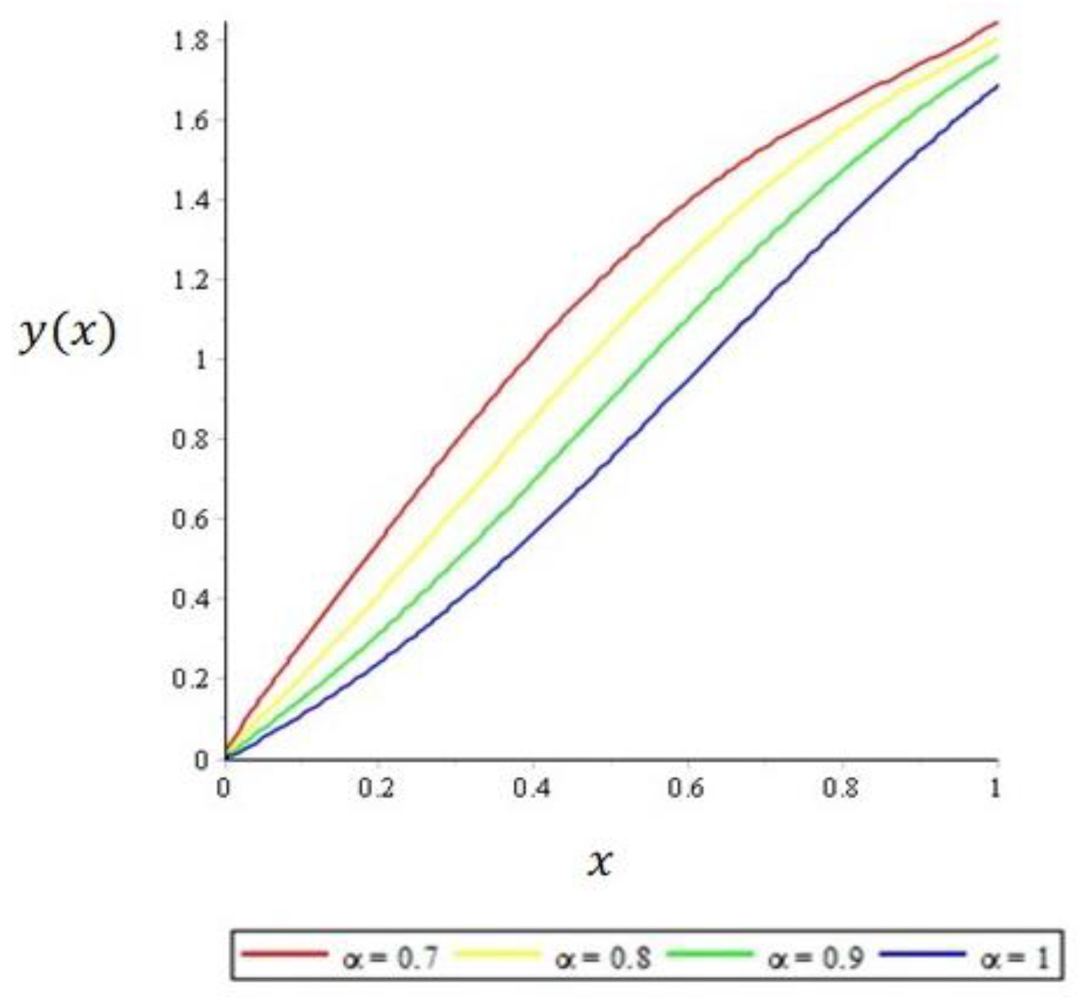
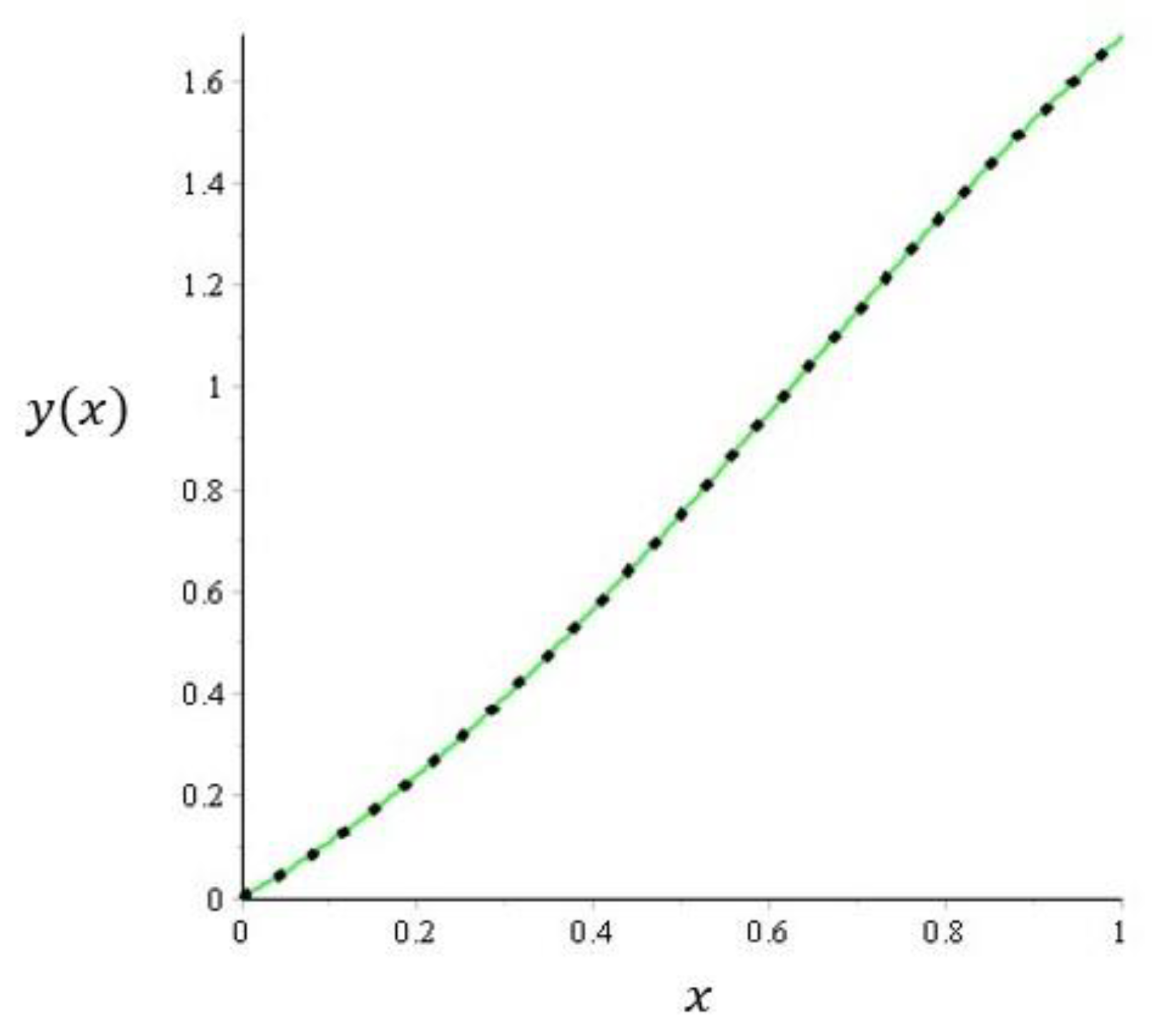
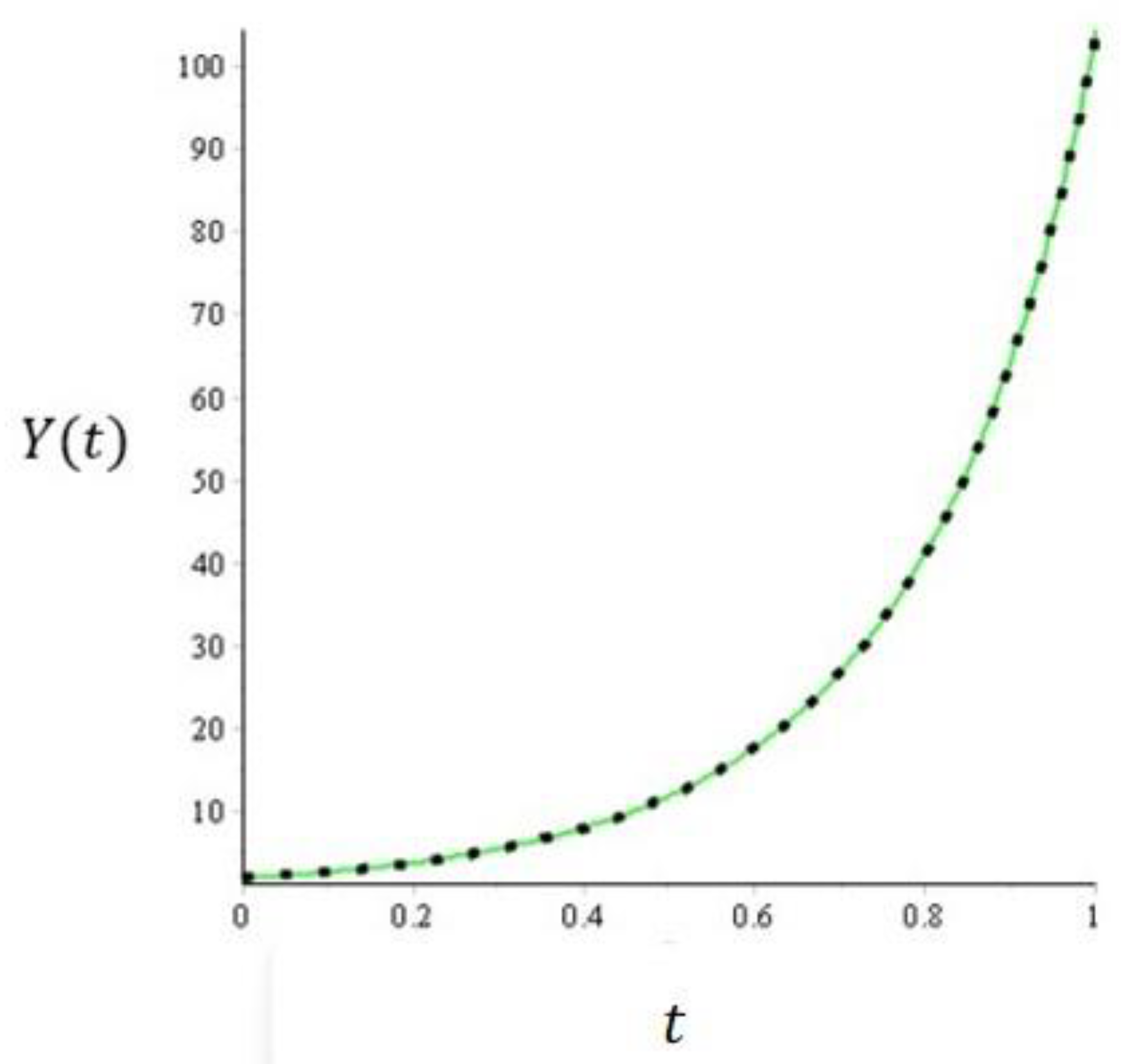
3.4. Numerical Simulation of Economic Growth Model Using ADM-Kamal Combined Method

Example 2.

 

Referring to the work by Johansyah et al. [2], the economic growth model involving memory effects has been presented as follows:

$$D_t^{\alpha }Y\left(t\right)=k_1{Y}^2\left(t\right)+k_{2}Y\left(t\right)+k_3,$$

(27)

where the order of the$\alpha$fractional derivative is the level of consumer memory loss of prices during a certain time interval and:

$$k_1=-\frac{ma}{v}, k_2=\frac{m\left(P-k\right)}{v}, k_3=f\left(t\right)=-\frac{mb}{v}.$$

We set$m=\frac{1}{4}$, P = 162,$a=-\frac{2}{5}$, b = 80, v = 10, k = 2, and the initial condition is$Y\left(0\right)=2$.

We obtained the exact solution as follows:

$$\begin{array}{c}\hfill Y\left(t\right)=\frac{10\sqrt{402}}{201}(-10\sqrt{402}\hfill \\ \hfill +201\tanh \left(\frac{\sqrt{402}}{2010}\left(5\sqrt{402}\mathrm{arctanh}\left(\frac{101}{2010}\sqrt{402}\right)-201t\right)\right)). \hfill \end{array}$$

(28)

Here we give the graph the RFDEapproximate solution Y(t) using the ADM-Kamal Combined Theorem for$\alpha =0.7; 0.8; 0.9, and 1$. Does the solution graph of the Y(t) approximation using the ADM-Kamal Combined Theorem for$\alpha =1$coincide with the exact solution (28)?

Answer

We calculate all values of k₁, k₂, and k₃ as follows:

$$\begin{array}{c}\hfill k_1=-\frac{ma}{v}=-\frac{\left(\frac{1}{4}\right)\left(-\frac{2}{5}\right)}{10}=0.01; \hfill \\ \hfill k_2=\frac{m\left(P-k\right)}{v}=\frac{\left(\frac{1}{4}\right)\left(162-2\right)}{10}=4; \hfill \\ \hfill k_3=-\frac{mb}{v}=-\frac{\left(\frac{1}{4}\right)\left(80\right)}{10}=-2.\hfill \end{array}$$

Thus, the RFDE in Equation (27) is as follows:

$$\begin{array}{c}\hfill D_t^{\alpha }Y(t)=k_1{Y}^2(t)+k_{2}Y(t)+k_3,\hfill \\ \hfill D_t^{\alpha }Y\left(t\right)=0.01Y^2\left(t\right)+4Y-2, t>0, 0<\alpha \le 1.\hfill \end{array}$$

(29)

Based on the ADM-Kamal Combined Theorem, the approximate solution of the RFDE (27) in the economic growth model, the output value is obtained as follows:

$$\begin{array}{cc}\hfill w_0& =w\left(0\right)+{\mathcal{G}}^{-1}\left[v^{\alpha }\mathcal{G}\left[P\right]\right],\hfill \\ \hfill w_{n+1}& ={\mathcal{G}}^{-1}\left[v^{\alpha }\mathcal{G}\left[Q{w}_n\right]\right]+{\mathcal{G}}^{-1}\left[v^{\alpha }\mathcal{G}\left[R{A}_n\right]\right],n=0,1,2,\dots ,\hfill \end{array}$$

with $R=k_1=0.01; Q=k_2=4; and P=k_3=-2$, we obtained:

$$\begin{array}{cc}{y}_0\hfill & =y\left(0\right)+{\mathcal{G}}^{-1}\left[v^{\alpha }\mathcal{G}\left[k_3\right]\right],\hfill \\ y_0\hfill & =2+{\mathcal{G}}^{-1}\left[v^{\alpha }\mathcal{G}\left[-2\right]\right],\hfill \\ y_0\hfill & =2-2{\mathcal{G}}^{-1}\left[v^{\alpha }v\right],\hfill \\ y_0\hfill & =2-2{\mathcal{G}}^{-1}\left[v^{\alpha +1}\right],\hfill \\ y_0\hfill & =2-\frac{2}{\mathsf{\Gamma }\left(\alpha +1\right)}{t}^{\alpha }.\hfill \\ y_{n+1}\hfill & ={\mathcal{G}}^{-1}\left[v^{\alpha }\mathcal{G}\left[k_2{y}_n\right]\right]+{\mathcal{G}}^{-1}\left[v^{\alpha }\mathcal{G}\left[k_1{A}_n\right]\right], n=0,1,2,\dots ,\hfill \\ y_{n+1}\hfill & ={\mathcal{G}}^{-1}\left[v^{\alpha }\mathcal{G}\left[4y_n\right]\right]+{\mathcal{G}}^{-1}\left[v^{\alpha }\mathcal{G}\left[0.01·A_n\right]\right],\hfill \\ y_{n+1}\hfill & =4{\mathcal{G}}^{-1}\left[v^{\alpha }\mathcal{G}\left[y_n\right]\right]+0.01{\mathcal{G}}^{-1}\left[v^{\alpha }\mathcal{G}\left[A_n\right]\right],\hfill \end{array}$$

(30)

where A_n is the Adomian polynomial of the nonlinear operator Ny = y², which can be described as follows:

$$\begin{array}{cc}{A}_0\hfill & =y_0^2,\hfill \\ A_1\hfill & =2y_0{y}_1,\hfill \\ A_2\hfill & =2y_0{y}_2+y_1^2,\hfill \\ ⋮\hfill & \end{array}$$

The following is a description of the approximate solution (30):

$$\begin{array}{cc}{y}_0\hfill & =2-\frac{2}{\mathsf{\Gamma }\left(\alpha +1\right)}{t}^{\alpha }.\hfill \\ y_{n+1}\hfill & =4{\mathcal{G}}^{-1}\left[v^{\alpha }\mathcal{G}\left[y_n\right]\right]+0.01{\mathcal{G}}^{-1}\left[v^{\alpha }\mathcal{G}\left[A_n\right]\right], n=0,1,2,\dots ,\hfill \\ y_1\hfill & =4{\mathcal{G}}^{-1}\left[v^{\alpha }\mathcal{G}\left[y_0\right]\right]+0.01{\mathcal{G}}^{-1}\left[v^{\alpha }\mathcal{G}\left[A_0\right]\right],\hfill \\ y_1\hfill & =4{\mathcal{G}}^{-1}\left[v^{\alpha }\mathcal{G}\left[2-\frac{2}{\mathsf{\Gamma }\left(\alpha +1\right)}{t}^{\alpha }\right]\right]+0.01{\mathcal{G}}^{-1}\left[v^{\alpha }\mathcal{G}\left[y_0^2\right]\right],\hfill \\ y_1\hfill & =4{\mathcal{G}}^{-1}\left[v^{\alpha }\mathcal{G}\left[2-\frac{2}{\mathsf{\Gamma }\left(\alpha +1\right)}{t}^{\alpha }\right]\right]+0.01{\mathcal{G}}^{-1}\left[v^{\alpha }\mathcal{G}\left[{\left(2-\frac{2}{\mathsf{\Gamma }\left(\alpha +1\right)}{t}^{\alpha }\right)}^2\right]\right],\hfill \\ y_1\hfill & =4{\mathcal{G}}^{-1}\left[v^{\alpha }\left(2v-2v^{\alpha +1}\right)\right]+0.01{\mathcal{G}}^{-1}\left[v^{\alpha }\mathcal{G}\left[4-\frac{8}{\mathsf{\Gamma }\left(\alpha +1\right)}{t}^{\alpha }+\frac{4}{{\mathsf{\Gamma }}^2\left(\alpha +1\right)}{t}^{2\alpha }\right]\right],\hfill \\ y_1\hfill & =4{\mathcal{G}}^{-1}\left[2v^{\alpha +1}-2v^{2\alpha +1}\right]+0.01{\mathcal{G}}^{-1}\left[v^{\alpha }\left(4v-8v^{\alpha +1}+\frac{4\mathsf{\Gamma }\left(2\alpha +1\right)}{{\mathsf{\Gamma }}^2\left(\alpha +1\right)}{v}^{2\alpha +1}\right)\right],\hfill \\ y_1\hfill & =8\left(\frac{1}{\mathsf{\Gamma }\left(\alpha +1\right)}{t}^{\alpha }-\frac{1}{\mathsf{\Gamma }\left(2\alpha +1\right)}{t}^{2\alpha }\right)\hfill \\ \hfill & +0.01{\mathcal{G}}^{-1}\left[4v^{\alpha +1}-8v^{2\alpha +1}+\frac{4\mathsf{\Gamma }\left(2\alpha +1\right)}{{\mathsf{\Gamma }}^2\left(\alpha +1\right)}{v}^{3\alpha +1}\right],\hfill \\ y_1\hfill & =\frac{8}{\mathsf{\Gamma }\left(\alpha +1\right)}{t}^{\alpha }-\frac{8}{\mathsf{\Gamma }\left(2\alpha +1\right)}{t}^{2\alpha }\hfill \\ \hfill & +0.01(\frac{4}{\mathsf{\Gamma }\left(\alpha +1\right)}{t}^{\alpha }-\frac{8}{\mathsf{\Gamma }\left(2\alpha +1\right)}{t}^{2\alpha }+\frac{4\mathsf{\Gamma }\left(2\alpha +1\right)}{{\mathsf{\Gamma }}^2\left(\alpha +1\right)\mathsf{\Gamma }\left(3\alpha +1\right)}{t}^{3\alpha }),\hfill \\ y_1\hfill & =\frac{8}{\mathsf{\Gamma }\left(\alpha +1\right)}{t}^{\alpha }-\frac{8}{\mathsf{\Gamma }\left(2\alpha +1\right)}{t}^{2\alpha }+\frac{0.04}{\mathsf{\Gamma }\left(\alpha +1\right)}{t}^{\alpha }-\frac{0.08}{\mathsf{\Gamma }\left(2\alpha +1\right)}{t}^{2\alpha }\hfill \\ \hfill & +\frac{0.04\mathsf{\Gamma }\left(2\alpha +1\right)}{{\mathsf{\Gamma }}^2\left(\alpha +1\right)\mathsf{\Gamma }\left(3\alpha +1\right)}{t}^{3\alpha },\hfill \\ y_1\hfill & =\frac{8.04}{\mathsf{\Gamma }\left(\alpha +1\right)}{t}^{\alpha }-\frac{8.08}{\mathsf{\Gamma }\left(2\alpha +1\right)}{t}^{2\alpha }+\frac{0.04\mathsf{\Gamma }\left(2\alpha +1\right)}{{\mathsf{\Gamma }}^2\left(\alpha +1\right)\mathsf{\Gamma }\left(3\alpha +1\right)}{t}^{3\alpha }.\hfill \\ y_{n+1}\hfill & =4{\mathcal{G}}^{-1}\left[v^{\alpha }\mathcal{G}\left[y_n\right]\right]+0.01{\mathcal{G}}^{-1}\left[v^{\alpha }\mathcal{G}\left[A_n\right]\right], n=0,1,2,\dots ,\hfill \\ y_2\hfill & =4{\mathcal{G}}^{-1}\left[v^{\alpha }\mathcal{G}\left[y_1\right]\right]+0.01{\mathcal{G}}^{-1}\left[v^{\alpha }\mathcal{G}\left[A_1\right]\right],\hfill \\ y_2\hfill & =4{\mathcal{G}}^{-1}\left[v^{\alpha }\mathcal{G}\left[\frac{8.04}{\mathsf{\Gamma }\left(\alpha +1\right)}{t}^{\alpha }-\frac{8.08}{\mathsf{\Gamma }\left(2\alpha +1\right)}{t}^{2\alpha }+\frac{0.04\mathsf{\Gamma }\left(2\alpha +1\right)}{{\mathsf{\Gamma }}^2\left(\alpha +1\right)\mathsf{\Gamma }\left(3\alpha +1\right)}{t}^{3\alpha }\right]\right]\hfill \\ \hfill & +0.01{\mathcal{G}}^{-1}\left[v^{\alpha }\mathcal{G}\left[2y_0{y}_1\right]\right],\hfill \\ y_2\hfill & =4{\mathcal{G}}^{-1}\left[v^{\alpha }\mathcal{G}\left[\frac{8.04}{\mathsf{\Gamma }\left(\alpha +1\right)}{t}^{\alpha }-\frac{8.08}{\mathsf{\Gamma }\left(2\alpha +1\right)}{t}^{2\alpha }+\frac{0.04\mathsf{\Gamma }\left(2\alpha +1\right)}{{\mathsf{\Gamma }}^2\left(\alpha +1\right)\mathsf{\Gamma }\left(3\alpha +1\right)}{t}^{3\alpha }\right]\right]\hfill \\ & +0.01{\mathcal{G}}^{-1}\left[v^{\alpha }\mathcal{G}\right[2\left(2-\frac{2}{\mathsf{\Gamma }\left(\alpha +1\right)}{t}^{\alpha }\right)(\frac{8.04}{\mathsf{\Gamma }\left(\alpha +1\right)}{t}^{\alpha }-\frac{8.08}{\mathsf{\Gamma }\left(2\alpha +1\right)}{t}^{2\alpha }\hfill \\ & +\frac{0.04\mathsf{\Gamma }\left(2\alpha +1\right)}{{\mathsf{\Gamma }}^2\left(\alpha +1\right)\mathsf{\Gamma }\left(3\alpha +1\right)}{t}^{3\alpha })]],\hfill \\ y_2\hfill & =4{\mathcal{G}}^{-1}\left[v^{\alpha }\left(8.04v^{\alpha +1}-8.08v^{2\alpha +1}+\frac{0.04\mathsf{\Gamma }\left(2\alpha +1\right)}{{\mathsf{\Gamma }}^2\left(\alpha +1\right)}{v}^{3\alpha +1}\right)\right]\hfill \\ \hfill & +0.01{\mathcal{G}}^{-1}\left[v^{\alpha }\mathcal{G}\right[\left(4-\frac{4}{\mathsf{\Gamma }\left(\alpha +1\right)}{t}^{\alpha }\right)(\frac{8.04}{\mathsf{\Gamma }\left(\alpha +1\right)}{t}^{\alpha }-\frac{8.08}{\mathsf{\Gamma }\left(2\alpha +1\right)}{t}^{2\alpha }\hfill \\ \hfill & +\frac{0.04\mathsf{\Gamma }\left(2\alpha +1\right)}{{\mathsf{\Gamma }}^2\left(\alpha +1\right)\mathsf{\Gamma }\left(3\alpha +1\right)}{t}^{3\alpha })]],\hfill \\ y_2\hfill & =4{\mathcal{G}}^{-1}\left[8.04v^{2\alpha +1}-8.08v^{3\alpha +1}+\frac{0.04\mathsf{\Gamma }\left(2\alpha +1\right)}{{\mathsf{\Gamma }}^2\left(\alpha +1\right)}{v}^{4\alpha +1}\right]\hfill \\ & +0.01{\mathcal{G}}^{-1}\left[v^{\alpha }\mathcal{G}\right[\frac{32.16}{\mathsf{\Gamma }(\alpha +1)}{t}^{\alpha }-\frac{32.32}{\mathsf{\Gamma }(2\alpha +1)}{t}^{2\alpha }+\frac{0.16\mathsf{\Gamma }(2\alpha +1)}{{\mathsf{\Gamma }}^2(\alpha +1)\mathsf{\Gamma }(3\alpha +1)}{t}^{3\alpha }\hfill \\ & -\frac{32.16}{\mathsf{\Gamma }(\alpha +1)\mathsf{\Gamma }(\alpha +1)}{t}^{\alpha }{t}^{\alpha }+\frac{32.32}{\mathsf{\Gamma }(2\alpha +1)\mathsf{\Gamma }(\alpha +1)}{t}^{2\alpha }{t}^{\alpha }\hfill \\ & -\frac{0.16\mathsf{\Gamma }(2\alpha +1)}{{\mathsf{\Gamma }}^2(\alpha +1)\mathsf{\Gamma }(3\alpha +1)\mathsf{\Gamma }(\alpha +1)}{t}^{3\alpha }{t}^{\alpha }\left]\right],\hfill \\ y_2\hfill & =4(\frac{8.04}{\mathsf{\Gamma }(2\alpha +1)}{t}^{2\alpha }-\frac{8.08}{\mathsf{\Gamma }(3\alpha +1)}{t}^{3\alpha }+\frac{0.04\mathsf{\Gamma }(2\alpha +1)}{{\mathsf{\Gamma }}^2(\alpha +1)\mathsf{\Gamma }(4\alpha +1)}{t}^{4\alpha })\hfill \\ & +0.01{\mathcal{G}}^{-1}\left[v^{\alpha }\mathcal{G}\right[\frac{32.16}{\mathsf{\Gamma }(\alpha +1)}{t}^{\alpha }-\frac{32.32}{\mathsf{\Gamma }(2\alpha +1)}{t}^{2\alpha }\hfill \\ & +\frac{0.16\mathsf{\Gamma }(2\alpha +1)}{{\mathsf{\Gamma }}^2(\alpha +1)\mathsf{\Gamma }(3\alpha +1)}{t}^{3\alpha }-\frac{32.32}{{\mathsf{\Gamma }}^2(\alpha +1)}{t}^{2\alpha }\hfill \\ & +\frac{32.32}{\mathsf{\Gamma }(2\alpha +1)\mathsf{\Gamma }(\alpha +1)}{t}^{3\alpha }-\frac{0.16\mathsf{\Gamma }(2\alpha +1)}{{\mathsf{\Gamma }}^3(\alpha +1)\mathsf{\Gamma }(3\alpha +1)}{t}^{4\alpha }\left]\right],\hfill \\ y_2\hfill & =\frac{32.16}{\mathsf{\Gamma }(2\alpha +1)}{t}^{2\alpha }-\frac{32.32}{\mathsf{\Gamma }(3\alpha +1)}{t}^{3\alpha }+\frac{0.16\mathsf{\Gamma }(2\alpha +1)}{{\mathsf{\Gamma }}^2(\alpha +1)\mathsf{\Gamma }(4\alpha +1)}{t}^{4\alpha }\hfill \\ & +0.01{\mathcal{G}}^{-1}\left[v^{\alpha }\right(32.16v^{\alpha +1}-32.32v^{2\alpha +1}+\frac{0.16\mathsf{\Gamma }(2\alpha +1)}{{\mathsf{\Gamma }}^2(\alpha +1)}{v}^{3\alpha +1}\hfill \\ & -\frac{32.16\mathsf{\Gamma }(2\alpha +1)}{{\mathsf{\Gamma }}^2(\alpha +1)}{v}^{2\alpha +1}+\frac{32.32\mathsf{\Gamma }(3\alpha +1)}{\mathsf{\Gamma }(2\alpha +1)\mathsf{\Gamma }(\alpha +1)}{v}^{3\alpha +1}\hfill \\ & -\frac{0.16\mathsf{\Gamma }(2\alpha +1)\mathsf{\Gamma }(4\alpha +1)}{{\mathsf{\Gamma }}^3(\alpha +1)\mathsf{\Gamma }(3\alpha +1)}{v}^{4\alpha +1}\left)\right],\hfill \\ y_2\hfill & =\frac{32.16}{\mathsf{\Gamma }(2\alpha +1)}{t}^{2\alpha }-\frac{32.32}{\mathsf{\Gamma }(3\alpha +1)}{t}^{3\alpha }+\frac{0.16\mathsf{\Gamma }(2\alpha +1)}{{\mathsf{\Gamma }}^2(\alpha +1)\mathsf{\Gamma }(4\alpha +1)}{t}^{4\alpha }\hfill \\ & +0.01{\mathcal{G}}^{-1}[32.16v^{2\alpha +1}-32.32v^{3\alpha +1}+\frac{0.16\mathsf{\Gamma }(2\alpha +1)}{{\mathsf{\Gamma }}^2(\alpha +1)}{v}^{4\alpha +1}\hfill \\ & -\frac{32.16\mathsf{\Gamma }(2\alpha +1)}{{\mathsf{\Gamma }}^2(\alpha +1)}{v}^{3\alpha +1}+\frac{32.32\mathsf{\Gamma }(3\alpha +1)}{\mathsf{\Gamma }(2\alpha +1)\mathsf{\Gamma }(\alpha +1)}{v}^{4\alpha +1}\hfill \\ & -\frac{0.16\mathsf{\Gamma }(2\alpha +1)\mathsf{\Gamma }(4\alpha +1)}{{\mathsf{\Gamma }}^3(\alpha +1)\mathsf{\Gamma }(3\alpha +1)}{v}^{5\alpha +1}],\hfill \\ y_2\hfill & =\frac{32.16}{\mathsf{\Gamma }(2\alpha +1)}{t}^{2\alpha }-\frac{32.32}{\mathsf{\Gamma }(3\alpha +1)}{t}^{3\alpha }+\frac{0.16\mathsf{\Gamma }(2\alpha +1)}{{\mathsf{\Gamma }}^2(\alpha +1)\mathsf{\Gamma }(4\alpha +1)}{t}^{4\alpha }\hfill \\ & +0.01(\frac{0.3216}{\mathsf{\Gamma }(2\alpha +1)}{t}^{2\alpha }-\frac{0.3232}{\mathsf{\Gamma }(3\alpha +1)}{t}^{3\alpha }+\frac{0.0016\mathsf{\Gamma }(2\alpha +1)}{{\mathsf{\Gamma }}^2(\alpha +1)\mathsf{\Gamma }(4\alpha +1)}{t}^{4\alpha }\hfill \\ & -\frac{32.16\mathsf{\Gamma }(2\alpha +1)}{{\mathsf{\Gamma }}^2(\alpha +1)\mathsf{\Gamma }(3\alpha +1)}{t}^{3\alpha }+\frac{32.32\mathsf{\Gamma }(3\alpha +1)}{\mathsf{\Gamma }(2\alpha +1)\mathsf{\Gamma }(\alpha +1)\mathsf{\Gamma }(4\alpha +1)}{t}^{4\alpha }\hfill \\ & -\frac{0.16\mathsf{\Gamma }(2\alpha +1)\mathsf{\Gamma }(4\alpha +1)}{{\mathsf{\Gamma }}^3(\alpha +1)\mathsf{\Gamma }(3\alpha +1)\mathsf{\Gamma }(5\alpha +1)}{t}^{5\alpha }),\hfill \\ y_2\hfill & =\frac{32.16}{\mathsf{\Gamma }(2\alpha +1)}{t}^{2\alpha }-\frac{32.32}{\mathsf{\Gamma }(3\alpha +1)}{t}^{3\alpha }+\frac{0.16\mathsf{\Gamma }(2\alpha +1)}{{\mathsf{\Gamma }}^2(\alpha +1)\mathsf{\Gamma }(4\alpha +1)}{t}^{4\alpha }+\frac{0.3216}{\mathsf{\Gamma }(2\alpha +1)}{t}^{2\alpha }\hfill \\ & -\frac{0.3232}{\mathsf{\Gamma }(3\alpha +1)}{t}^{3\alpha }+\frac{0.0016\mathsf{\Gamma }(2\alpha +1)}{{\mathsf{\Gamma }}^2(\alpha +1)\mathsf{\Gamma }(4\alpha +1)}{t}^{4\alpha }\hfill \\ & -\frac{0.3216\mathsf{\Gamma }(2\alpha +1)}{{\mathsf{\Gamma }}^2(\alpha +1)\mathsf{\Gamma }(3\alpha +1)}{t}^{3\alpha }+\frac{0.3232\mathsf{\Gamma }(3\alpha +1)}{\mathsf{\Gamma }(2\alpha +1)\mathsf{\Gamma }(\alpha +1)\mathsf{\Gamma }(4\alpha +1)}{t}^{4\alpha }\hfill \\ & -\frac{0.0016\mathsf{\Gamma }(2\alpha +1)\mathsf{\Gamma }(4\alpha +1)}{{\mathsf{\Gamma }}^3(\alpha +1)\mathsf{\Gamma }(3\alpha +1)\mathsf{\Gamma }(5\alpha +1)}{t}^{5\alpha },\hfill \\ y_2\hfill & =\frac{32.4816}{\mathsf{\Gamma }(2\alpha +1)}{t}^{2\alpha }-\frac{32.6432}{\mathsf{\Gamma }(3\alpha +1)}{t}^{3\alpha }+\frac{0.16\mathsf{\Gamma }(2\alpha +1)}{{\mathsf{\Gamma }}^2(\alpha +1)\mathsf{\Gamma }(4\alpha +1)}{t}^{4\alpha }\hfill \\ & +\frac{0.0016\mathsf{\Gamma }(2\alpha +1)}{{\mathsf{\Gamma }}^2(\alpha +1)\mathsf{\Gamma }(4\alpha +1)}{t}^{4\alpha }-\frac{0.3216\mathsf{\Gamma }(2\alpha +1)}{{\mathsf{\Gamma }}^2(\alpha +1)\mathsf{\Gamma }(3\alpha +1)}{t}^{3\alpha }\hfill \\ & +\frac{0.3232\mathsf{\Gamma }(3\alpha +1)}{\mathsf{\Gamma }(2\alpha +1)\mathsf{\Gamma }(\alpha +1)\mathsf{\Gamma }(4\alpha +1)}{t}^{4\alpha }\hfill \\ & -\frac{0.0016\mathsf{\Gamma }(2\alpha +1)\mathsf{\Gamma }(4\alpha +1)}{{\mathsf{\Gamma }}^3(\alpha +1)\mathsf{\Gamma }(3\alpha +1)\mathsf{\Gamma }(5\alpha +1)}{t}^{5\alpha }.\hfill \\ y\left(t\right)\hfill & =y_0+y_1+y_2+\dots ,\hfill \\ & =2-\frac{2}{\mathsf{\Gamma }(\alpha +1)}{t}^{\alpha }+\frac{8.04}{\mathsf{\Gamma }(\alpha +1)}{t}^{\alpha }-\frac{8.08}{\mathsf{\Gamma }(2\alpha +1)}{t}^{2\alpha }+\frac{0.04\mathsf{\Gamma }(2\alpha +1)}{{\mathsf{\Gamma }}^2(\alpha +1)\mathsf{\Gamma }(3\alpha +1)}{t}^{3\alpha }\hfill \\ & +\frac{32.4816}{\mathsf{\Gamma }(2\alpha +1)}{t}^{2\alpha }-\frac{32.6432}{\mathsf{\Gamma }(3\alpha +1)}{t}^{3\alpha }+\frac{0.16\mathsf{\Gamma }(2\alpha +1)}{{\mathsf{\Gamma }}^2(\alpha +1)\mathsf{\Gamma }(4\alpha +1)}{t}^{4\alpha }\hfill \\ & +\frac{0.0016\mathsf{\Gamma }(2\alpha +1)}{{\mathsf{\Gamma }}^2(\alpha +1)\mathsf{\Gamma }(4\alpha +1)}{t}^{4\alpha }-\frac{0.3216\mathsf{\Gamma }(2\alpha +1)}{{\mathsf{\Gamma }}^2(\alpha +1)\mathsf{\Gamma }(3\alpha +1)}{t}^{3\alpha }\hfill \\ & +\frac{0.3232\mathsf{\Gamma }(3\alpha +1)}{\mathsf{\Gamma }(2\alpha +1)\mathsf{\Gamma }(\alpha +1)\mathsf{\Gamma }(4\alpha +1)}{t}^{4\alpha }\hfill \\ & -\frac{0.0016\mathsf{\Gamma }(2\alpha +1)\mathsf{\Gamma }(4\alpha +1)}{{\mathsf{\Gamma }}^3(\alpha +1)\mathsf{\Gamma }(3\alpha +1)\mathsf{\Gamma }(5\alpha +1)}{t}^{5\alpha }\hfill \\ & +\dots .\hfill \end{array}$$

(31)

Figure 3 displays the graph of the exact solution of Equation (28) (green line) coinciding with the graph of the approximate solution using ADM-Kamal Combined Method (black dot) for $\alpha =1$ in $0<t\le 1$. It shows that the ADM-Kamal Combined Method is very accurate, it is also easy to use to solve RFDE on the economic growth model.

The numerical simulation results in

Table 1. The exact solution for the economic growth model using ADM-Kamal Combined Theorem for $\alpha =0.7; 0.8; 0.9; \mathrm{and} 1$.

$\mathit{t}$	Approximate Solution
	$\mathit{\alpha }\mathbf{=}\mathbf{0.7}$	$\mathit{\alpha }\mathbf{=}\mathbf{0.8}$	$\mathit{\alpha }\mathbf{=}\mathbf{0.9}$	$\mathit{\alpha }\mathbf{=}\mathbf{1}$
0	2	2	2	2
0.2	9.687973998	6.260302407	4.710244008	3.861227413
0.4	46.21972094	19.56419792	11.57216925	8.074385875
0.6	328.0381130	69.24841234	30.29195286	17.79339967
0.8	3635.669747	331.8435757	87.92003272	41.22290131
1	38,049.84591	2366.054814	321.7714120	103.9547603

show that for t, the closer to 1, the output value Y(t) gets bigger, while for $\alpha$ getting closer to 1, the output value Y(t) gets smaller. The output value of Y(t) will be maximum if the value of $\alpha$ is close to zero for the value of t = 1. Based on this, the memory effect significantly affects the output value of Y(t) for the quadratic cost function in the economic growth model.

In this paper, we have proposed RFDE on an economic growth model involving memory effects for the quadratic cost function. The value a, k < 0 is defined as the marginal cost reduction at the output value Y(t) of a, k. Meanwhile, if the value of a, k = 0, then there is no additional cost or marginal cost reduction of a, k and if a, k > 0, then there is an additional marginal cost at the output value of Y(t) of a, k.

4. Conclusions

In this paper, we have proved the existence and uniqueness of the RFDE solution with constant coefficients with the help of Banach’s fixed point theorem (contraction theorem). The main novelty of this work was to investigate the existence and uniqueness of the non-linear RFDE with constant coefficients in the economic growth model. The RFDE approximate solution to the economic growth model involving memory effect has been completed with ADM-Kamal Combined Theorem. Furthermore, the graph of the exact solution coincides with the graph of the approximate for $\alpha$ = 1 with 0 < t $\le$ 1. The results of the numerical simulation showed that the output value for t was getting closer to 1, then the output value of Y(t) was getting bigger, while for $\alpha$ was getting closer to 1. The output value of Y(t) was getting smaller. The ADM-Kamal Combined Method is accurate and efficient for solving RFDE on economic growth models.

References

1. Johansyah, M.D.; Supriatna, A.K.; Rusyaman, E.; Saputra, J. Application of fractional differential equation in economic growth model: A systematic review approach. AIMS Math. 2021, 6, 10266–10280. [Google Scholar] [CrossRef]
2. Johansyah, M.D.; Supriatna, A.K.; Rusyaman, E.; Saputra, J. Solving the Economic Growth Acceleration Model with Memory Effects: An Application of Combined Theorem of Adomian Decomposition Methods and Kashuri–Fundo Transformation Methods. Symmetry 2022, 14, 192. [Google Scholar] [CrossRef]
3. Sukono; Sambas, A.; He, S.; Liu, H.; Vaidyanathan, S.; Hidayat, Y.; Saputra, J. Dynamical analysis and adaptive fuzzy control for the fractional-order financial risk chaotic system. Adv. Differ. Equ. 2020, 2020, 674. [Google Scholar] [CrossRef]
4. Subartini, B.; Vaidyanathan, S.; Sambas, A.; Zhang, S. Multistability in the Finance Chaotic System, Its Bifurcation Analysis and Global Chaos Synchronization via Integral Sliding Mode Control. IAENG Int. J. Appl. Math. 2021, 51, 995–1002. [Google Scholar]
5. Xin, B.; Zhang, J. Finite-time stabilizing a fractional-order chaotic financial system with market confidence. Nonlinear Dyn. 2015, 79, 1399–1409. [Google Scholar] [CrossRef]
6. Jia, H.; Pu, Y. Fractional calculus method for enhancing digital image of bank slip. Congr. Image Signal Process. 2008, 3, 326–330. [Google Scholar]
7. Chen, T.; Wang, D. Combined application of blockchain technology in fractional calculus model of supply chain financial system. Chaos Solitons Fractals 2020, 131, 109461. [Google Scholar] [CrossRef]
8. Wang, W.; Khan, M.A.; Kumam, P.; Thounthong, P. A comparison study of bank data in fractional calculus. Chaos Solitons Fractals 2019, 126, 369–384. [Google Scholar] [CrossRef]
9. Tenreiro Machado, J.A.; Lopes, A.M. Relative fractional dynamics of stock markets. Nonlinear Dyn. 2016, 86, 1613–1619. [Google Scholar] [CrossRef]
10. Sambas, A.; Vaidyanathan, S.; Zhang, X.; Koyuncu, I.; Bonny, T.; Tuna, M.; Alcin, M.; Zhang, S.; Sulaiman, I.M.; Awwal, A.M.; et al. A Novel 3D Chaotic System with Line Equilibrium: Multistability, Integral Sliding Mode Control, Electronic Circuit, FPGA and its Image Encryption. IEEE Access 2022, 10, 68057–68074. [Google Scholar] [CrossRef]
11. Sambas, A.; Vaidyanathan, S.; Tlelo-Cuautle, E.; Abd-El-Atty, B.; Abd El-Latif, A.A.; Guillen-Fernandez, O.; Sukono; Hidayat, Y.; Gundara, G. A 3-D multi-stable system with a peanut-shaped equilibrium curve: Circuit design, FPGA realization, and an application to image encryption. IEEE Access 2020, 8, 137116–137132. [Google Scholar]
12. Vaidyanathan, S.; Sambas, A.; Mamat, M.; Sanjaya, W.S.M. A new three-dimensional chaotic system with a hidden attractor, circuit design and application in wireless mobile robot. Arch. Control. Sci. 2017, 27, 541–554. [Google Scholar]
13. Silva-Juárez, A.; Tlelo-Cuautle, E.; De La Fraga, L.G.; Li, R. FPAA-based implementation of fractional-order chaotic oscillators using first-order active filter blocks. J. Adv. Res. 2020, 25, 77–85. [Google Scholar]
14. Sambas, A.; Vaidyanathan, S.; Bonny, T.; Zhang, S.; Hidayat, Y.; Gundara, G.; Mamat, M. Mathematical model and FPGA realization of a multi-stable chaotic dynamical system with a closed butterfly-like curve of equilibrium points. Appl. Sci. 2021, 11, 788. [Google Scholar] [CrossRef]
15. Karakaya, B.; Gülten, A.; Frasca, M. A true random bit generator based on a memristive chaotic circuit: Analysis, design and FPGA implementation. Chaos Solitons Fractals 2019, 119, 143–149. [Google Scholar]
16. Wazwaz, A.M. The combined Laplace transform–Adomian decomposition method for handling nonlinear Volterra integro–differential equations. Appl. Math. Comput. 2010, 216, 1304–1309. [Google Scholar]
17. Babolian, E.; Vahidi, A.R.; Shoja, A. An efficient method for nonlinear fractional differential equations: Combination of the Adomian decomposition method and spectral method. Indian J. Pure Appl. Math. 2014, 45, 1017–1028. [Google Scholar]
18. Varsoliwala, A.C.; Singh, T.R. An approximate analytical solution of non linear partial differential equation for water infiltration in unsaturated soils by combined Elzaki Transform and Adomian Decomposition Method. J. Phys. Conf. Ser. 2020, 1473, 012009. [Google Scholar]
19. Ahmed, S.; Elzaki, T. The solution of nonlinear Volterra integro-differential equations of second kind by combine Sumudu transforms and Adomian decomposition method. Int. J. Adv. Innov. Res. 2013, 2, 90–93. [Google Scholar]
20. Chindhe, A.D.; Kiwne, S.B. Application of Combine Natural Transform and Adomian Decomposition Method in Volterra Integro-Differential Equations. Math. J. Interdiscip. Sci. 2016, 5, 1–14. [Google Scholar]
21. Johansyah, M.D.; Supriatna, A.K.; Rusyaman, E.; Saputra, J. Solving Differential Equations of Fractional Order Using Combined Adomian Decomposition Method with Kamal Integral Transformation. Math. Stat. 2022, 10, 187–194. [Google Scholar] [CrossRef]
22. Ramezani, M.; Nourazar, S.S.; Dehghanpour, H. Combination of Adomian decomposition method with Fourier transform for solving the squeezing flow influenced by a magnetic field. AUT J. Model. Simul. 2021, 53, 1–25. [Google Scholar]
23. Liaqat, M.I.; Khan, A.; Alam, M.; Pandit, M.K.; Etemad, S.; Rezapour, S. Approximate and closed-form solutions of Newell-Whitehead-Segel equations via modified conformable Shehu transform decomposition method. Math. Probl. Eng. 2022, 2022, 6752455. [Google Scholar]
24. Khandelwal, R.; Khandelwal, Y. Solution of Blasius Equation Concerning with Mohand Transform. Int. J. Appl. Comput. Math. 2020, 6, 128. [Google Scholar]
25. Diethelm, K.; Ford, N.J. Analysis of fractional differential equations. J. Math. Anal. Appl. 2002, 265, 229–248. [Google Scholar] [CrossRef]
26. Lakshmikantham, V.; Vatsala, A.S. Basic theory of fractional differential equations. Nonlinear Anal. Theory Methods Appl. 2008, 69, 2677–2682. [Google Scholar] [CrossRef]
27. Benlabbes, A.; Benbachir, M.; Lakrib, M. Existence solutions of a nonlinear fractional differential equations. J. Adv. Res. Dyn. Control. Syst. 2014, 6, 10266–10280. [Google Scholar]
28. Elsaid, A.; Latif, M.A.; Kamal, F.M. Series solution for fractional Riccati differential equation and its convergence. J. Fract. Calc. Appl. 2015, 6, 186–196. [Google Scholar]
29. Asaduzzaman, M.; Ali, M.Z. Existence of Multiple Positive Solutions to the Caputo-Type Nonlinear Fractional Differential Equation With Integral Boundary Value Conditions. Fixed Point Theory 2022, 23, 127–129. [Google Scholar]
30. Asaduzzaman, M.; Ali, M.Z. Existence of positive solution to the boundary value problems for coupled system of nonlinear fractional differential equations. AIMS Math. 2019, 4, 880–895. [Google Scholar]
31. Asaduzzaman, M.; Ali, M.Z. Existence of Triple Positive Solutions for Nonlinear Second Order Arbitrary Two-point Boundary Value Problems. Malays. J. Math. Sci. 2020, 14, 335–349. [Google Scholar]
32. Asaduzzaman, M.; Kilicman, A.; Ali, M.Z.; Sapar, S.H. Fixed point theorem based solvability of 2-Dimensional dissipative cubic nonlinear Klein-Gordon equation. Mathematics 2020, 8, 1103. [Google Scholar] [CrossRef]
33. El-Sayed, A.M.A.; El-Mesiry, A.E.M.; El-Saka, H.A.A. On the fractional-order logistic equation. Appl. Math. Lett. 2007, 20, 817–823. [Google Scholar]
34. Bartle, R.G.; Sherbert, D.R. Introduction to Real Analysis, 4th ed.; John Wiley & Sons: New York, NY, USA, 2011. [Google Scholar]
35. Mathai, A.M.; Haubold, H.J. An Introduction to Fractional Calculus; Nova Science Publishers: New York, NY, USA, 2017. [Google Scholar]
36. Kamal, A.; Sedeeg, H. The new integral transform Kamal transform. Adv. Theor. Appl. Math. 2016, 11, 451–458. [Google Scholar]
37. Wazwaz, A.M.; El-Sayed, S.M. A new modification of the Adomian decomposition method for linear and nonlinear operators. Appl. Math. Comput. 2001, 122, 393–405. [Google Scholar]
38. Odetunde, O.S.; Taiwo, O.A. A decomposition algorithm for the solution of fractional quadratic Riccati differential equations with Caputo derivatives. Am. J. Comput. Appl. Math. 2014, 4, 83–91. [Google Scholar]
Figure 1. Graphics of RFDE solution using the ADM-Kamal Combined Theorem (26) for α = 0.7 ,   α = 0.8 ,   α = 0.9 , and α = 1 .
Mathematics 10 03029 g001
Figure 2. The exact solution Odetunde and Taiwo [38] (green line) coincides with the approximate solution using the ADM-Kamal Combined Method (black dot) for α = 1.
Mathematics 10 03029 g002
Figure 3. The exact solution Equation (28) (green line) coincides with the approximate solution using the ADM-Kamal Combined Theorem for parameter α = 1 (black dot).
Mathematics 10 03029 g003