Efficient Estimation of Two-Parameter Xgamma Distribution Parameters Using Ranked Set Sampling Design

Abstract

An efficient method such as ranked set sampling is used for estimating the population parameters when the actual observation measurement is expensive and complicated. In this paper, we consider the problem of estimating the two-parameter xgamma (TPXG) distribution parameters under the ranked set sampling as well as the simple random sampling design. Various estimation methods, including the weighted least-square estimator, maximum likelihood estimators, least-square estimator, Cramer–von Mises, the maximum product of spacings estimators, and Anderson–Darling estimators, are considered. A comparison between the ranked set sampling and simple random sampling estimators, with the same number of measurement units, is conducted using a simulation study in terms of the bias, mean squared errors, and efficiency of estimators. The merit of the ranked set sampling estimators is examined using real data of bank customers. The results indicate that estimations using the ranked set sampling method are more efficient than the simple random sampling competitor considered in this study.

1. Introduction

A random variable X follows the xgamma distribution if its probability density function (pdf) is given by

$$f(x,\lambda )={\displaystyle \frac{{\lambda }^2\left(\lambda x^2+2\right)}{2\left(\lambda +1\right)}}{\mathrm{e}}^{-\lambda x};x>0,\lambda >0,$$

(1)

and its cumulative distribution function (CDF) is

$$F(x,\lambda )=1-{\displaystyle \frac{\frac{x^2{\lambda }^2}{2}+x\lambda +\lambda +1}{\lambda +1}}{\mathrm{e}}^{-x\lambda };x>0,\lambda >0.$$

(2)

Plots of the pdf of the xgamma distribution are presented in Figure 1 for some values of $\lambda$.

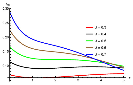
Figure 1. The pdfs plots of the xgamma distribution for different values of the $\lambda$.

As an extension to the xgamma distribution, the two-parameter xgamma distribution is proposed as a new distribution by [1] by using an additional parameter to the xgamma distribution to obtain a more flexible distribution in modeling real data sets due to the wide use of the xgamma distribution in several survival analyses. When a random variable, X, follows the TPXG distribution, the probability density function and the cumulative distribution function are, respectively, given by

$$f(x,\beta ,\lambda )={\displaystyle \frac{{\lambda }^2\left(\beta \lambda x^2+2\right){\mathrm{e}}^{-\lambda x}}{2\left(\lambda +\beta \right)}};x>0,\lambda >0,\beta >0,$$

(3)

$$F(x,\beta ,\lambda )=1-{\displaystyle \frac{\left(\frac{\beta x^2{\lambda }^2}{2}+\beta x\lambda +\lambda +\beta \right){\mathrm{e}}^{-x\lambda }}{\lambda +\beta }};x>0,\lambda >0,\beta >0.$$

(4)

For $\beta =1$ in (3), we obtain the xgamma distribution with parameter $\lambda$ as a special case of the TPXG distribution.

The rth moment for the distribution is obtained by

$$E\left(X^r\right)=\frac{r!}{2{\lambda }^r(\beta +\lambda )}[2\lambda +\beta (1+r)(2+r)];r=1,2\dots$$

(5)

The characteristic function (CF) and hazard function $H(x,\beta ,\lambda )$ of the model are, respectively, given by

$${\varphi }_X\left(t\right)=E\left[e^{itx}\right]=\frac{{\lambda }^2}{\beta +\lambda }\left[{(\lambda -it)}^{-1}+\beta \lambda {(\lambda -it)}^{-3}\right];t\in \mathbb{R},i=\sqrt{-1}.$$

(6)

$$H(x,\beta ,\lambda )=\frac{{\lambda }^2\left(\beta \lambda x^2+2\right)}{2\lambda +\beta \left(\lambda x\right(\lambda x+2)+2)}.$$

(7)

Figure 2 represents some possible pdf shapes of the TPXG distribution for selected values of $\beta$ and $\lambda$, which reveals the flexibility of the distribution in modeling right-skewed observations. Further, Figure 3 indicates the possible shapes of the function $H(x,\beta ,\lambda )$. They are bathtub, increasing, decreasing, and decreasing-increasing shapes. For more explanations regarding the TPXG distribution, see [1].

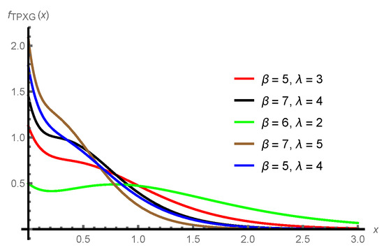
Figure 2. The pdfs plots of the TPXG distribution for different values of the parameters.

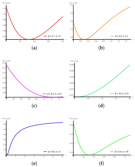
Figure 3. Plots of $H(x,\beta ,\lambda )$ of the TPXG distribution for (a) $\beta =2.1,\lambda =3$, (b) $\beta =2.2,\lambda =4$, (c) $\beta =0.3,\lambda =2.5$, (d) $\beta =10,\lambda =0.3$, (e) $\beta =9.9,\lambda =5$, (f) $\beta =0.9,\lambda =16$.

When the variable of interest is expensive to measure or difficult to obtain, but cheap and simple to rank, ranked set sampling is recognized as an effective sampling strategy for enhancing the accuracy and efficiency of parameters estimation. McIntyre [2] proposed the ranked set sampling scheme for estimating the pasture and forage yields.

Let $X\sim$TPXG distribution, with the pdfs $f\left(x\right)$ and CDF $F\left(x\right)$, where $\mu$ and ${\sigma }^2$ represent, respectively, the population mean and variance. Let the random sample $X_1$, $X_2$, ⋯, $X_k$$(i=1,2,\cdots ,k)$ with the same pdf $f\left(x\right)$. The method of the ranked set sampling (RSS) can be described as follows:

• Choose k simple random sampling (SRS) each of size k (set size) from the underlying population as

  $X_{1\left(1k\right)}$,	$X_{1\left(2k\right)}$,	…,	$X_{1\left(kk\right)}$.
  $X_{2\left(1k\right)}$,	$X_{2\left(2k\right)}$,	…,	$X_{2\left(kk\right)}$.
  ⋮	⋮	⋮	⋮
  $X_{k\left(1k\right)}$,	$X_{k\left(2k\right)}$,	…,	$X_{k\left(kk\right)}.$

• Rank the units in each set of size k from lowest to the largest visually or based on any cost-free method as

  $X_{1(1:k)}$,	$X_{1(2:k)}$,	…,	$X_{1(k:k)}$.
  $X_{2(1:k)}$,	$X_{2(2:k)}$,	…,	$X_{2(k:k)}$.
  ⋮	⋮	⋮	⋮
  $X_{k(1:k)}$,	$X_{k(2:k)}$,	…,	$X_{k(k:k)}.$

• Select the ith order statistic (in bold) from the ith set ($i=1$, 2, …, k) as

  ${\mathit{X}}_{\mathbf{1}(\mathbf{1}:\mathit{k})}$,	$X_{1(2:k)}$,	…,	$X_{1(k:k)}$.
  $X_{2(1:k)}$,	${\mathit{X}}_{\mathbf{2}(\mathbf{2}:\mathit{k})}$,	…,	$X_{2(k:k)}$.
  ⋮	⋮	⋮	⋮
  $X_{k(1:k)}$,	$X_{k(2:k)}$,	…,	${\mathit{X}}_{\mathit{k}(\mathit{k}:\mathit{k})}$.

• Repeat the Steps (1)–(3), n times (cycles) to obtain an RSS of size $N=kn$.

The selected RSS units are denoted by $X_{1(1:k)},X_{2(2:k)},\dots ,X_{k(k:k)}$, where $X_{j(i:k)}$ is the ith largest unit in a set of size k in the jth cycle. Notice that even we selected $k^2$ units, we only measured k of them; these units are not identically distributed, but they are independent because they are selected from different sets.

Takahasi and Wakimoto [3] delivered the mathematical theory of the RSS, and showed that the RSS estimator of mean with the perfect ranking is unbiased and better than the SRS estimator due to its smaller variance. The SRS mean estimator is given by

$${\displaystyle {\overline{X}}_{SRS}=\frac{1}{k}\sum _{i=1}^k{X}_i, \mathrm{with}\mathrm{variance} \mathrm{Var}\left({\overline{X}}_{SRS}\right)=\frac{{\sigma }^2}{k}.}$$

The RSS estimator of the population mean with its variance are given by

$${\displaystyle {\overline{X}}_{RSS}=\frac{1}{nk}\sum _{j=1}^n\sum _{i=1}^k{X}_{j(i:k)},}$$

$${\displaystyle \mathrm{Var}\left({\overline{X}}_{RSS}\right)=\frac{1}{n{k}^2}\sum _{i=1}^k{\displaystyle \mathrm{Var}\left(X_{(i:k)}\right)=\frac{{\sigma }^2}{nk}-\frac{1}{n{k}^2}\sum _{i=1}^k{\left({\mu }_{(i:k)}-\mu \right)}^2}.}$$

Note that since $\frac{1}{k^2}{\sum }_{i=1}^k{({\mu }_{(i:k)}-\mu )}^2\ge 0$, we have

$$\mathrm{Var}\left({\overline{X}}_{RSS}\right)\le \mathrm{Var}\left({\overline{X}}_{SRS}\right).$$

They also showed that

$${\displaystyle \mu =\frac{1}{k}\sum _{i=1}^k{\mu }_{(i:k)} \mathrm{and} f\left(x\right)=\frac{1}{k}\sum _{i=1}^k{f}_{(i:k)\left(x\right)},}$$

where

$${\displaystyle {\mu }_{(i:k)}=\underset{-\infty }{\overset{\infty }{\int }}x{f}_{(i:k)}\left(x\right)dx, \mathrm{and} {\sigma }_{(i:k)}^2={\int }_{-\infty }^{\infty }{\left(x-{\mu }_{(i:k)}\right)}^2{f}_{(i:k)}\left(x\right)dx.}$$

Under perfect rankings, this relation emphasizes the efficiency of the ${\overline{X}}_{RSS}$ mean estimator due to its variance compared to ${\overline{X}}_{SRS}$ for the SRS estimator for the same number of quantified observations regardless of the distribution of nature. Even with a ranking error, Dell and Clutter [4] demonstrated that RSS is more effective than simple random sampling.

Some further modifications of RSS are suggested in the literature, such as extreme RSS by Samawi et al. [5], Mutllak [6] introduced a modification of RSS called median ranked set sampling; another scheme of RSS is proposed by Al-Saleh and Al-Kadiri [7] which is the double RSS, percentile RSS by Mutllak [8], L RSS by Al-Nasser [9], Haq et al. [10] suggested partial RSS design, and neoteric RSS by Zamanzade and Al-Omari [11]. In addition to these modifications, many authors investigated the parameter estimation of some distributions using RSS or its modifications. For example, the logistic model parameters are estimated based on SRS and RSS by Abu-Dayyeh et al. [12]. The generalized quasi-Lindley distribution parameter estimation is considered by Al-Omari et al. [13]. Yousef and Al-Subh [14] used maximum likelihood methods to estimate Gumbel parameters under RSS. Akgul and Şenoglu [15] investigated some modifications of the RSS in estimating the Weibull distribution parameters. The Bayesian and maximum likelihood estimation approaches are considered by Hussian [16] to determine parameter estimates for the Kumaraswamy distribution under RSS. Chen et al. [17] used moving extremes RSS to estimate the scale parameter for the scale distribution. Al-Omari and Bouza [18] considered ratio estimators of the population mean with missing values using RSS. Later, Al-Omari [19] considered the varied L RSS and used the MLE in location-scale families. Hassan et al. [20] used median RSS and estimated the stress–strength reliability for the generalized inverted exponential distribution.

Due to the importance of the TPXG distribution in lifetime distributions and to our knowledge, this is the first study to consider the RSS design for parameter estimations of the TPXG distribution. Hence, the main focus of this paper is to use RSS design for estimating the TPXG distribution parameters and then use some well-known methods of estimation, including the method of maximum product of spacings, maximum likelihood method, ordinary least square method, method of Cramer and von Mises, weight least square method, and the Anderson–Darling method. Then, the suggested estimators based on the RSS design are compared with their competitors in SRS for the same number of measured observations. A real data set is analyzed to explain the usefulness of the offered estimators. Based on the gained results, the RSS estimators are found to be better than the SRS counterparts in terms of the MSE, bias, and efficiency values for all methods of estimation considered in the study.

The layout of this paper is as follows. The estimation methods of the TPXG distribution parameters are presented in Section 2. A simulation study is conducted to show the superiority of the RSS relative to the SRS estimators in Section 3. In Section 4, the suggested estimators’ usefulness is examined using a real data set fitted to the TPXG distribution. The last section will present the conclusion and remarks.

2. Method of Estimation

Here, based on RSS design, six estimation methods are considered to estimate the $\lambda$ and $\beta$ parameters of the TPXG distribution, which are: the maximum likelihood (MLE) method, the maximum product of spacings (MPS) method, ordinary least square (OLS) method, weight least square (WLS) method, Cramer–von Mises (CV) method, and Anderson–Darling (AD) method. In all methods, we denote by $\{X_{(i:k)j},i=1,2,\dots ,$k$; j=1,2,\dots ,n\}$ the ith order statistics from the ith set of size k of the jth cycle and take them to be the RSS data for X with sample size $N=kn$.

2.1. MLE Method

Considering an RSS sample of size $N=kn$, the likelihood function is obtained by

$$M_{RSS}(\beta ,\lambda )=\prod _{j=1}^r\prod _{i=1}^k{f}_{(i:k)}(x_{(i:k)j},\beta ,\lambda ),$$

(8)

with

$$\begin{array}{ccc}\hfill f_{(i:k)}(x_{(i:k)j},\beta ,\lambda )& =& {\displaystyle \frac{k!}{(i-1)!(k-i)!}{\left[F\left(x_{(i:k)j}\right)\right]}^{i-1}{[1-F\left(x_{(i:k)j}\right)]}^{k-i}f\left(x_{(i:k)j}\right)}\hfill \\ \hfill & =& {\displaystyle \frac{k!}{(i-1)!(k-i)!}{\left[1-{\displaystyle \frac{{\mathrm{e}}^{-\lambda x_{(i:k)j}}\left(\frac{{\lambda }^2{x}_{(i:k)j}^2\beta }{2}+\lambda x_{(i:k)j}\beta +\beta +\lambda \right)}{\beta +\lambda }}\right]}^{i-1}}\hfill \\ \hfill & \times & {\left[{\displaystyle \frac{{\mathrm{e}}^{-\lambda x_{(i:k)j}}\left(\frac{{\lambda }^2{x}_{(i:k)j}^2\beta }{2}+\lambda x_{(i:k)j}\beta +\beta +\lambda \right)}{\beta +\lambda }}\right]}^{k-i}\hfill \\ \hfill & \times & \left({\displaystyle \frac{{\lambda }^2\left(\beta \lambda x_{(i:k)j}^2+2\right){\mathrm{e}}^{-\lambda x_{(i:k)j}}}{2\left(\lambda +\beta \right)}}\right).\hfill \end{array}$$

(9)

Let the log-likelihood function ${\Psi }_{RSS}=log{M}_{RSS}(\beta ,\lambda )$ be

$$\begin{array}{ccc}\hfill {\Psi }_{RSS}& =& \sum _{j=1}^r\sum _{i=1}^{k}log\left\{f_{(i:k)}(x_{(i:k)j},\lambda ,\beta )\right\}\hfill \\ \hfill & =& \sum _j^r\sum _{i=1}^{k}log\left({\displaystyle \frac{k!}{(i-1)!(k-i)!}}\right)+\sum _{j=1}^r\sum _{i=1}^k(i-1)log\left(F\left(x_{(i:k)j}\right)\right)\hfill \\ \hfill & +& \sum _{j=1}^r\sum _{i=1}^k(k-i)log(1-F\left(x_{(i:k)j}\right))+\sum _{j=1}^r\sum _{i=1}^{k}logf\left(x_{(i:k)j}\right).\hfill \end{array}$$

(10)

The $\frac{\partial {\Psi }_{RSS}}{\partial \lambda }=0$ and $\frac{\partial {\Psi }_{RSS}}{\partial \beta }=0$ cannot be obtained explicitly and they are not in closed form. Hence, they should be solved numerically to find the MLEs, ${\widehat{\lambda }}_{RSS}^{MLE}$ and ${\widehat{\beta }}_{RSS}^{MLE}$ of $\lambda$ and $\beta$, respectively.

2.2. Method of MPS

Cheng and Amin [21,22] introduced this method, which depends on maximizing the geometric mean of data spacings. Consider $X_{(1:N)},X_{(2:N)},\dots ,X_{(N:N)}$ to be an ordered sample forming a RSS of size $N=nk$ from the TPXG distribution. The uniform spacings are given by

$${\upsilon }_i(\beta ,\lambda )=F\left(x_{(i:N)}\right|\beta ,\lambda )-F\left(x_{(i-1:N)}\right|\beta ,\lambda ),i=1,2,\cdots ,N.$$

Note that $F\left(x_{0:N}\right|\beta ,\lambda )=0$ and $F\left(x_{N+1:N}\right|\beta ,\lambda )=1$. It is clear that ${\displaystyle \sum _{i=1}^{N+1}{\upsilon }_i(\beta ,\lambda )=1.}$

Let the geometric mean of the spacing be

$$Q(\beta ,\lambda |\mathrm{x})={\left[\prod _{i=1}^{N+1}{\upsilon }_i(\beta ,\lambda )\right]}^{\frac{1}{N+1}}.$$

(11)

The natural logarithm of (11) is

$${\rm Y}(\beta ,\lambda |\mathrm{x})=\frac{1}{N+1}\sum _{i=1}^{N+1}log{\upsilon }_i(\beta ,\lambda ).$$

The estimators, ${\widehat{\beta }}_{RSS}^{MPS}$ and ${\widehat{\lambda }}_{RSS}^{MPS}$, are the values of $\beta$ and $\lambda$, which maximize the geometric mean of spacings. The determination of these estimators can be achieved by determining the solution of the following nonlinear equations:

$$\frac{\partial }{\partial \beta }{\rm Y}(\beta ,\lambda )=\frac{1}{N+1}\sum _{i=1}^{N+1}\frac{1}{{\upsilon }_i(\beta ,\lambda )}\left[{\Phi }_1\left(x_{(i:N)}\right|\beta ,\lambda )-{\Phi }_1\left(x_{(i-1:N)}\right|\beta ,\lambda )\right]=0,$$

$$\frac{\partial }{\partial \lambda }{\rm Y}(\beta ,\lambda )=\frac{1}{N+1}\sum _{i=1}^{N+1}\frac{1}{{\upsilon }_i(\beta ,\lambda )}\left[{\Phi }_2\left(x_{(i:N)}\right|\beta ,\lambda )-{\Phi }_2\left(x_{(i-1:N)}\right|\beta ,\lambda )\right]=0,$$

where

$${\Phi }_1\left(x_{(i:N)}\right|\beta ,\lambda )=\frac{\partial }{\partial \beta }F\left(x_{(i:N)}\right|\beta ,\lambda )=-{\displaystyle \frac{{\lambda }^2{x}_{(i:N)}·\left(\lambda x_{(i:N)}+2\right){\mathrm{e}}^{-\lambda x_{(i:N)}}}{2{\left(\beta +\lambda \right)}^2}},$$

(12)

and

$${\Phi }_2\left(x_{(i:N)}\right|\beta ,\lambda )=\frac{\partial }{\partial \lambda }F\left(x_{(i:N)}\right|\beta ,\lambda )={\displaystyle \frac{x_{(i:N)}\lambda ·\left(\beta x_{(i:N)}^2{\lambda }^2+\left({\beta }^2{x}_{(i:N)}^2+\beta x_{(i:N)}+2\right)\lambda +4\beta \right){\mathrm{e}}^{-x_{(i:N)}\lambda }}{2{\left(\lambda +\beta \right)}^2}},$$

(13)

that can be solved numerically.

2.3. Methods of LS

Well-known results in probability theory indicate that $F\left(x_{(i:N)}\right)\sim Beta(i,N-i+1)$, where F is a distribution function, and $X_{(i:N)}$ are the ith-order statistic of the sample $\left(X_1,X_2,\dots ,X_N\right)$. Therefore, ${\displaystyle E\left[F\left(x_{(i:N)}\right)\right]=\frac{i}{N+1}}$ and ${\displaystyle \mathrm{V}\mathrm{a}\mathrm{r}\left[F\left(x_{(i:N)}\right)\right]=\frac{i(N-i+1)}{{(N+1)}^2(N+2)}}$.

Using the expectation and variance, two variants of the least squares methods can be obtained. Swain et al. [23] were the first to use the method of LS for parameter estimations of the beta distribution.

2.3.1. OLS Method

The OLS estimators ${\widehat{\beta }}_{OLS}^{RSS}$ and ${\widehat{\lambda }}_{OLS}^{RSS}$ of $\beta$ and $\lambda$, respectively, can be found by minimizing the following function, with respect to $\beta$ and $\lambda$:

$$\begin{array}{ccc}\hfill \Omega (\beta ,\lambda |\mathrm{x})& =& \sum _{i=1}^N{\left[F\left(x_{(i:N)}\right|\beta ,\lambda )-\frac{i}{N+1}\right]}^2\hfill \\ & =& \hfill \sum _{i=1}^N{\left[1-{\displaystyle \frac{\left(\frac{\beta x_{(i:N)}^2{\lambda }^2}{2}+\beta x_{(i:N)}\lambda +\lambda +\beta \right){\mathrm{e}}^{-x_{(i:N)}\lambda }}{\lambda +\beta }}-\frac{i}{N+1}\right]}^2,\hfill \end{array}$$

Alternatively, we can obtain the estimators by solving simultaneously the nonlinear equations:

$$\sum _{i=1}^N\left[F\left(x_{(i:N)}\right|\beta ,\lambda )-\frac{i}{N+1}\right]{\Phi }_1\left(x_{(i:N)}\right|\beta ,\lambda )=0,$$

$$\sum _{i=1}^N\left[F\left(x_{(i:N)}\right|\beta ,\lambda )-\frac{i}{N+1}\right]{\Phi }_2\left(x_{(i:N)}\right|\beta ,\lambda )=0,$$

where ${\Phi }_1\left(x_{(i:N)}\right|\beta ,\lambda )$ and ${\Phi }_2\left(x_{(i:N)}\right|\beta ,\lambda )$ are defined as in (12) and (13), respectively.

2.3.2. WLS Method

The WLS estimators of $\beta$ and $\lambda$, say, ${\widehat{\beta }}_{WLS}^{RSS}$ and ${\widehat{\lambda }}_{WLS}^{RSS}$, respectively, can be determined by minimizing the following function, with respect to $\beta$ and $\lambda$:

$$\begin{array}{ccc}\hfill W(\beta ,\lambda |\mathrm{x})& =& \sum _{i=1}^N\frac{{(N+1)}^2(N+2)}{i(N-i+1)}{\left[F\left(x_{(i:N)}\right|\beta ,\lambda )-\frac{i}{N+1}\right]}^2\hfill \\ & =& \sum _{i=1}^N\frac{{(N+1)}^2(N+2)}{i(N-i+1)}\hfill \\ & & {\left[1-{\displaystyle \frac{\left(\frac{\beta x_{(i:N)}^2{\lambda }^2}{2}+\beta x_{(i:N)}\lambda +\lambda +\beta \right){\mathrm{e}}^{-x_{(i:N)}\lambda }}{\lambda +\beta }}-\frac{i}{N+1}\right]}^2,\hfill \end{array}$$

Note that these estimators are also the solution to the following nonlinear equations:

$$\sum _{i=1}^N\frac{{(N+1)}^2(N+2)}{i(N-i+1)}\left[F\left(x_{(i:N)}\right|\beta ,\lambda )-\frac{i}{N+1}\right]{\Phi }_1\left(x_{(i:N)}\right|\beta ,\lambda )=0,$$

$$\sum _{i=1}^N\frac{{(N+1)}^2(N+2)}{i(N-i+1)}\left[F\left(x_{(i:N)}\right|\beta ,\lambda )-\frac{i}{N+1}\right]{\Phi }_2\left(x_{(i:N)}\right|\beta ,\lambda )=0,$$

where ${\Phi }_1\left(x_{(i:N)}\right|\beta ,\lambda )$ and ${\Phi }_2\left(x_{(i:N)}\right|\beta ,\lambda )$ are specified as in (12) and (13), respectively.

2.4. Methods of Minimum Distances

Several methods of estimation can be proposed based on the minimization of test statistics between the empirical cumulative distribution and theoretical functions. The Cramer–von Mises and Anderson–Darling methods are considered here. (See D’Agostino and Stephens [24]).

2.4.1. CV Method

The CV ${\widehat{\beta }}_{CV}^{RSS}$ and ${\widehat{\lambda }}_{CV}^{RSS}$ of $\beta$ and $\lambda$, respectively, can be found by minimizing the following function, with respect to $\beta$ and $\lambda$:

$$\begin{array}{ccc}\hfill CV(\beta ,\lambda )& =& \frac{1}{12N}+\sum _{i=1}^N\frac{{(N+1)}^2(N+2)}{i(N-i+1)}{\left[F(x_{(i:N)};\beta ,\lambda )-\frac{2i-1}{2N}\right]}^2\hfill \\ & =& \frac{1}{12N}+\sum _{i=1}^N\frac{{(N+1)}^2(N+2)}{i(N-i+1)}\hfill \\ & & {\left[1-{\displaystyle \frac{\left(\frac{\beta x_{(i:N)}^2{\lambda }^2}{2}+\beta x_{(i:N)}\lambda +\lambda +\beta \right){\mathrm{e}}^{-x_{(i:N)}\lambda }}{\lambda +\beta }}-\frac{2i-1}{2N}\right]}^2,\hfill \end{array}$$

Consequently, these estimators are also the solution to the nonlinear equations:

$$\sum _{i=1}^N\frac{{(N+1)}^2(N+2)}{i(N-i+1)}\left[F\left(x_{(i:N)}\right|\beta ,\lambda )-\frac{2i-1}{2N}\right]{\Phi }_1\left(x_{(i:N)}\right|\beta ,\lambda )=0,$$

$$\sum _{i=1}^N\frac{{(N+1)}^2(N+2)}{i(N-i+1)}\left[F\left(x_{(i:N)}\right|\beta ,\lambda )-\frac{2i-1}{2N}\right]{\Phi }_2\left(x_{(i:N)}\right|\beta ,\lambda )=0,$$

where ${\Phi }_1\left(x_{(i:N)}\right|\beta ,\lambda )$ and ${\Phi }_2\left(x_{(i:N)}\right|\beta ,\lambda )$ are given in (12) and (13), respectively.

2.4.2. AD Method

The AD estimates of the TPXG distribution parameters, $\beta$ and $\lambda$, denoted by ${\widehat{\beta }}_{AD}^{RSS}$ and ${\widehat{\lambda }}_{AD}^{RSS}$, can be gained by minimizing the following function with respect to $\beta$ and $\lambda$:

$$\begin{array}{ccc}\hfill A(\beta ,\lambda )& =& -N-\frac{1}{N}\sum _{i=1}^N(2i-1)\{logF\left(x_{(i:N)}\right|\beta ,\lambda )+log\overline{F}\left(x_{(N-i+1:N)}\right|\beta ,\lambda )\},\hfill \\ & =& -N-\frac{1}{N}\sum _{i=1}^N(2i-1)\left\{log\left(1-{\displaystyle \frac{\left(\frac{\beta x_{(i:N)}^2{\lambda }^2}{2}+\beta x_{(i:N)}\lambda +\lambda +\beta \right){\mathrm{e}}^{-x_{(i:N)}\lambda }}{\lambda +\beta }}\right)\right.\hfill \\ & +& \left.log\left({\displaystyle \frac{\left(\frac{\beta x_{(i:N)}^2{\lambda }^2}{2}+\beta x_{(i:N)}\lambda +\lambda +\beta \right){\mathrm{e}}^{-x_{(i:N)}\lambda }}{\lambda +\beta }}\right)\right\},\hfill \end{array}$$

or by simultaneously solving the two equations:

$$\frac{\partial A(\beta ,\lambda )}{\partial \beta }=\sum _{i=1}^N(2i-1)\left\{\frac{{\Phi }_1\left(x_{(i:N)}\right|\beta ,\lambda )}{F\left(x_{(i:N)}\right|\beta ,\lambda )}-\frac{{\Phi }_1\left(x_{(N-i+1:N)}\right|\beta ,\lambda )}{\overline{F}\left(x_{(N-i+1:N)}\right|\beta ,\lambda )}\right\}=0,$$

and

$$\frac{\partial A(\beta ,\lambda )}{\partial \lambda }=\sum _{i=1}^N(2i-1)\left\{\frac{{\Phi }_2\left(x_{(i:N)}\right|\beta ,\lambda )}{F\left(x_{(i:N)}\right|\beta ,\lambda )}-\frac{{\Phi }_2\left(x_{(N-i+1:N)}\right|\beta ,\lambda )}{\overline{F}\left(x_{(N-i+1:N)}\right|\beta ,\lambda )}\right\}=0,$$

where ${\Phi }_1\left(x_{(i:N)}\right|\beta ,\lambda )$ and ${\Phi }_2\left(x_{(i:N)}\right|\beta ,\lambda )$ are specified in (12) and (13), respectively.

3. Simulation and Discussion

In this section, a simulation study is supplemented using R software. Based on different parameters and sample sizes for both designs RSS and SRS, 1000 samples from the TPXG distribution are generated. The simulation is performed assuming that the ranking in RSS design is perfect, i.e., there is no error in ranking. The number of cycles is nominated to be n = 10, 15, and 20, while the set size k is designated as 4, 5, and 6. The SRS size is $N=nk$, which must have the same size in the RSS design. For the purpose of comparison between SRS and RSS methods, the estimated mean squared error (MSE) and efficiency are deliberated for each estimator as:

$${\displaystyle MSE\left(\widehat{\beta }\right)=\frac{1}{1000}\sum _{i=1}^{1000}{\left(\widehat{{\beta }_i}-\beta \right)}^2\mathrm{and}MSE\left(\widehat{\lambda }\right)=\frac{1}{1000}\sum _{i=1}^{1000}{\left(\widehat{{\lambda }_i}-\lambda \right)}^2,}$$

where $\widehat{{\beta }_i}$ and $\widehat{{\lambda }_i}$ denote the estimate of $\beta$ and $\lambda$, respectively, for the ith simulated sample. The efficiency (Eff) values of the RSS estimators with respect to the SRS estimators based on the same sample size are defined by

$${\displaystyle Eff\left({\widehat{\beta }}_{RSS},{\widehat{\beta }}_{SRS}\right)=\frac{MSE\left({\widehat{\beta }}_{SRS}\right)}{MSE\left({\widehat{\beta }}_{RSS}\right)}\mathrm{and}Eff\left({\widehat{\lambda }}_{RSS}{\widehat{\lambda }}_{SRS}\right)=\frac{MSE\left({\widehat{\lambda }}_{SRS}\right)}{MSE\left({\widehat{\lambda }}_{RSS}\right)}.}$$

For various selections of the parameters, sample sizes and number of cycles, the estimates (ES), estimated MSE, and the Eff values are displayed in Table 1, Table 2, Table 3 and Table 4. The results in Table 1, Table 2, Table 3 and Table 4 indicate that:

Table 1. The ESs, MSEs, and Effs values, using the MLE, MPS, and OLS methods for the TPXG model parameters with $\beta =1$, $\lambda =1$.

n	k		Sampling	WLS			CV			AD
				Es	MSE	Eff	Es	MSE	Eff	Es	MSE	Eff
10	4	$\widehat{\beta }$	RSS	1.2822	0.8970	2.8395	0.8920	0.6166	1.7305	1.1081	1.0136	3.0978
			SRS	1.5018	2.5471		1.0348	1.0670		1.3057	3.1398
		$\widehat{\lambda }$	RSS	1.0047	0.0334	1.4867	0.8837	0.0634	0.9157	0.9463	0.0463	1.1537
			SRS	1.0068	0.0497		0.9034	0.0580		0.9652	0.0534
	5	$\widehat{\beta }$	RSS	1.2051	0.6485	3.9544	0.8959	0.4766	1.9883	1.0803	0.7148	1.7602
			SRS	1.4297	2.5644		1.0264	0.9476		1.1959	1.2582
		$\widehat{\lambda }$	RSS	1.0014	0.0248	1.7205	0.9038	0.0494	1.0278	0.9571	0.0357	1.2049
			SRS	1.0092	0.0426		0.9180	0.0508		0.9668	0.0430
	6	$\widehat{\beta }$	RSS	1.1811	0.4284	2.8285	0.8814	0.4284	1.6333	1.0526	0.5138	1.9028
			SRS	1.3048	1.2117		0.9809	0.6997		1.1567	0.9777
		$\widehat{\lambda }$	RSS	1.0096	0.0191	1.7311	0.9056	0.0479	0.9760	0.9650	0.0292	1.2111
			SRS	1.0038	0.0331		0.9164	0.0468		0.9679	0.0354
15	4	$\widehat{\beta }$	RSS	1.1980	0.5220	2.2403	0.9327	0.5051	1.3842	1.0614	0.6018	1.7132
			SRS	1.3315	1.1693		1.0131	0.6992		1.1728	1.0311
		$\widehat{\lambda }$	RSS	1.0092	0.0212	1.5417	0.9217	0.0406	1.0995	0.9574	0.0349	1.0294
			SRS	1.0055	0.0327		0.9208	0.0447		0.9660	0.0359
	5	$\widehat{\beta }$	RSS	1.1279	0.3831	2.1394	0.8883	0.3730	1.4622	1.0363	0.4818	1.2633
			SRS	1.2233	0.8196		0.9746	0.5454		1.0954	0.6086
		$\widehat{\lambda }$	RSS	0.9978	0.0183	1.6681	0.9139	0.0413	0.9143	0.9613	0.0281	1.1134
			SRS	0.9979	0.0305		0.9294	0.0378		0.9698	0.0313
	6	$\widehat{\beta }$	RSS	1.1102	0.2367	2.6970	0.9008	0.2436	1.9160	1.0101	0.2857	1.9564
			SRS	1.1833	0.6385		0.9750	0.4667		1.0864	0.5590
		$\widehat{\lambda }$	RSS	1.0057	0.0117	2.2664	0.9359	0.0284	1.1122	0.9710	0.0185	1.3982
			SRS	0.9989	0.0265		0.9414	0.0316		0.9743	0.0259
20	4	$\widehat{\beta }$	RSS	1.1535	0.3851	1.9453	0.9291	0.3667	1.4194	1.0485	0.4412	1.5535
			SRS	1.2323	0.7492		0.9926	0.5205		1.1359	0.6854
		$\widehat{\lambda }$	RSS	1.0044	0.0162	1.9553	0.9295	0.0331	1.0839	0.9692	0.0226	1.2817
			SRS	1.0022	0.0317		0.9378	0.0359		0.9811	0.0290
	5	$\widehat{\beta }$	RSS	1.1147	0.2362	2.0681	0.9290	0.2482	1.5216	1.0338	0.2807	1.5711
			SRS	1.1584	0.4885		0.9638	0.3777		1.0708	0.4410
		$\widehat{\lambda }$	RSS	1.0070	0.0127	1.6004	0.9438	0.0273	1.0055	0.9785	0.0178	1.2573
			SRS	1.0004	0.0202		0.9440	0.0275		0.9764	0.0224
	6	$\widehat{\beta }$	RSS	1.0709	0.1626	2.0186	0.8982	0.2007	1.3866	1.0067	0.2140	1.5474
			SRS	1.1306	0.3282		0.9637	0.2783		1.0749	0.3312
		$\widehat{\lambda }$	RSS	1.0014	0.0090	1.9698	0.9407	0.0242	0.9670	0.9770	0.0145	1.3105
			SRS	0.9999	0.0177		0.9507	0.0234		0.9833	0.0191

Table 2. The ESs, MSEs, and Effs values, using the WLS, CV, and AD methods for the TPXG model parameters with $\beta =1$, $\lambda =1$.

n	k		Sampling	WLS			CV			AD
				Es	MSE	Eff	Es	MSE	Eff	Es	MSE	Eff
10	4	$\widehat{\beta }$	RSS	1.1454	0.9627	2.3971	1.5024	1.8420	3.2663	1.1809	0.9235	2.1388
			SRS	1.3323	2.3077		1.7892	6.0165		1.3746	1.9752
		$\widehat{\lambda }$	RSS	0.9609	0.0421	1.1735	1.0297	0.0423	1.2695	0.9736	0.0387	1.1148
			SRS	0.9744	0.0494		1.0472	0.0537		0.9922	0.0432
	5	$\widehat{\beta }$	RSS	1.1085	0.6941	2.0320	1.3873	1.1647	2.1187	1.1458	0.6652	2.0651
			SRS	1.2510	1.4103		1.5651	2.4676		1.2897	1.3736
		$\widehat{\lambda }$	RSS	0.9673	0.0331	1.1906	1.0285	0.0308	1.3332	0.9814	0.0302	1.2161
			SRS	0.9787	0.0394		1.0360	0.0411		0.9918	0.0368
	6	$\widehat{\beta }$	RSS	1.0850	0.4915	2.0535	1.3100	0.7583	2.1090	1.1209	0.4893	2.0556
			SRS	1.2145	1.0093		1.4627	1.5993		1.2373	1.0057
		$\widehat{\lambda }$	RSS	0.9762	0.0265	1.2298	1.0270	0.0253	1.3354	0.9881	0.0239	1.2891
			SRS	0.9821	0.0326		1.0299	0.0338		0.9907	0.0308
15	4	$\widehat{\beta }$	RSS	1.1145	0.6484	1.6197	1.3426	0.9927	1.6418	1.1437	0.6288	1.6188
			SRS	1.2299	1.0501		1.4819	1.6299		1.2535	1.0180
		$\widehat{\lambda }$	RSS	0.9744	0.0300	1.0810	1.0242	0.0288	1.0940	0.9860	0.0273	1.0980
			SRS	0.9803	0.0325		1.0307	0.0315		0.9901	0.0299
	5	$\widehat{\beta }$	RSS	1.0646	0.4564	1.4143	1.2430	0.6365	1.4503	1.0849	0.4309	1.5054
			SRS	1.1370	0.6454		1.3234	0.9232		1.1551	0.6487
		$\widehat{\lambda }$	RSS	0.9727	0.0243	1.1433	1.0149	0.0222	1.2360	0.9817	0.0220	1.2253
			SRS	0.9813	0.0278		1.0227	0.0275		0.9868	0.0270
	6	$\widehat{\beta }$	RSS	1.0434	0.2625	2.1830	1.1862	0.3523	2.1911	1.0684	0.2629	2.1731
			SRS	1.1253	0.5731		1.2787	0.7720		1.1383	0.5713
		$\widehat{\lambda }$	RSS	0.9837	0.0148	1.5218	1.0179	0.0142	1.5458	0.9917	0.0139	1.5096
			SRS	0.9869	0.0225		1.0213	0.0219		0.9922	0.0209
20	4	$\widehat{\beta }$	RSS	1.0801	0.4347	1.6750	1.2440	0.6007	1.7131	1.1011	0.4327	1.5615
			SRS	1.1784	0.7281		1.3568	1.0291		1.1902	0.6757
		$\widehat{\lambda }$	RSS	0.9805	0.0192	1.3983	1.0180	0.0185	1.4710	0.9872	0.0186	1.3114
			SRS	0.9922	0.0268		1.0299	0.0272		0.9988	0.0244
	5	$\widehat{\beta }$	RSS	1.0636	0.2655	1.6645	1.1930	0.3442	1.6822	1.0815	0.2660	1.6672
			SRS	1.1058	0.4420		1.2412	0.5789		1.1190	0.4434
		$\widehat{\lambda }$	RSS	0.9891	0.0154	1.2095	1.0205	0.0147	1.2242	0.9952	0.0143	1.2327
			SRS	0.9882	0.0187		1.0197	0.0180		0.9933	0.0176
	6	$\widehat{\beta }$	RSS	1.0288	0.1928	1.6684	1.1372	0.2353	1.7142	1.0399	0.1849	1.7156
			SRS	1.1003	0.3217		1.2134	0.4034		1.1086	0.3172
		$\widehat{\lambda }$	RSS	0.9857	0.0122	1.3090	1.0137	0.0103	1.4823	0.9909	0.0105	1.4428
			SRS	0.9921	0.0159		1.0190	0.0153		0.9956	0.0151

Table 3. The ESs, MSEs, and Effs values, using the MLE, MPS, and OLS methods for the TPXG model parameters with $\beta =0.5$, $\lambda =1$.

n	k		Sampling	WLS			CV			AD
				Es	MSE	Eff	Es	MSE	Eff	Es	MSE	Eff
10	4	$\widehat{\beta }$	RSS	0.7681	0.5863	2.2926	0.5127	0.3742	1.5608	0.6942	0.6792	2.6051
			SRS	0.9016	1.3442		0.5843	0.5840		0.8047	1.7693
		$\widehat{\lambda }$	RSS	1.0360	0.0620	1.3453	0.9025	0.0693	1.0132	0.9991	0.0637	1.0801
			SRS	1.0377	0.0834		0.9191	0.0702		1.0145	0.0688
	5	$\widehat{\beta }$	RSS	0.6968	0.3947	2.4677	0.4768	0.2587	1.6924	0.6606	0.6318	1.5033
			SRS	0.8374	0.9740		0.5557	0.4377		0.7878	0.9498
		$\widehat{\lambda }$	RSS	1.0178	0.0501	1.3100	0.9006	0.0606	0.9538	0.9906	0.0543	1.1423
			SRS	1.0307	0.0657		0.9180	0.0578		1.0233	0.0621
	6	$\widehat{\beta }$	RSS	0.6098	0.2167	2.8960	0.4166	0.1611	2.1658	0.5591	0.2968	2.9335
			SRS	0.7601	0.6277		0.5380	0.3489		0.7358	0.8708
		$\widehat{\lambda }$	RSS	0.9988	0.0377	1.6417	0.8850	0.0538	1.0265	0.9655	0.0417	1.3349
			SRS	1.0188	0.0619		0.9239	0.0552		1.0193	0.0557
15	4	$\widehat{\beta }$	RSS	0.6983	0.3494	2.2947	0.4895	0.2550	1.7792	0.6871	0.5204	1.5954
			SRS	0.7781	0.8019		0.5512	0.4536		0.7432	0.8303
		$\widehat{\lambda }$	RSS	1.0250	0.0471	1.3393	0.9096	0.0586	0.9504	1.0109	0.0499	1.1248
			SRS	1.0144	0.0631		0.9207	0.0557		1.0107	0.0561
	5	$\widehat{\beta }$	RSS	0.6096	0.2053	2.1409	0.4248	0.1514	1.8825	0.5678	0.2570	1.8184
			SRS	0.7203	0.4395		0.5275	0.2851		0.6802	0.4673
		$\widehat{\lambda }$	RSS	1.0050	0.0346	1.5334	0.8974	0.0496	1.0226	0.9786	0.0398	1.1677
			SRS	1.0199	0.0530		0.9288	0.0507		1.0109	0.0465
	6	$\widehat{\beta }$	RSS	0.5897	0.1523	1.8181	0.4284	0.1324	1.5013	0.5633	0.2184	1.5977
			SRS	0.6301	0.2769		0.4694	0.1987		0.6517	0.3489
		$\widehat{\lambda }$	RSS	1.0036	0.0296	1.6904	0.9046	0.0458	1.0519	0.9821	0.0363	1.1660
			SRS	0.9933	0.0501		0.9143	0.0482		1.0135	0.0424
20	4	$\widehat{\beta }$	RSS	0.6063	0.2237	1.9466	0.4384	0.1759	1.6529	0.5971	0.2924	1.7466
			SRS	0.6894	0.4354		0.5116	0.2908		0.6850	0.5108
		$\widehat{\lambda }$	RSS	0.9997	0.0381	1.4077	0.9002	0.0521	0.9707	0.9888	0.0445	1.0531
			SRS	1.0064	0.0536		0.9233	0.0506		1.0114	0.0469
	5	$\widehat{\beta }$	RSS	0.5680	0.1270	2.1627	0.4230	0.1169	1.6505	0.5458	0.1715	2.1895
			SRS	0.6540	0.2748		0.4952	0.1930		0.6669	0.3756
		$\widehat{\lambda }$	RSS	0.9949	0.0270	1.6691	0.9043	0.0426	1.0178	0.9770	0.0329	1.2466
			SRS	1.0024	0.0450		0.9259	0.0434		1.0113	0.0411
	6	$\widehat{\beta }$	RSS	0.5427	0.1049	1.7870	0.4128	0.1099	1.3755	0.5235	0.1592	1.5091
			SRS	0.5791	0.1874		0.4514	0.1512		0.5718	0.2402
		$\widehat{\lambda }$	RSS	0.9880	0.0259	1.3978	0.9052	0.0419	0.9497	0.9698	0.0325	1.0423
			SRS	0.9838	0.0362		0.9149	0.0398		0.9822	0.0339

Table 4. The ESs, MSEs, and Effs values, using the WLS, CV, and AD methods for the TPXG model parameters with $\beta =0.5$, $\lambda =1$.

n	k		Sampling	WLS			CV			AD
				Es	MSE	Eff	Es	MSE	Eff	Es	MSE	Eff
10	4	$\widehat{\beta }$	RSS	0.6874	0.6705	1.5521	0.9502	1.3324	2.3410	0.7076	0.6432	2.2283
			SRS	0.7857	1.0407		1.0935	3.1191		0.8293	1.4332
		$\widehat{\lambda }$	RSS	0.9904	0.0638	1.0474	1.0713	0.0823	1.0847	1.0036	0.0633	1.0894
			SRS	1.0097	0.0668		1.0827	0.0893		1.0255	0.0689
	5	$\widehat{\beta }$	RSS	0.6412	0.4921	2.1837	0.8443	0.8789	2.1745	0.6547	0.4471	1.8495
			SRS	0.8065	1.0747		1.0407	1.9112		0.8052	0.8269
		$\widehat{\lambda }$	RSS	0.9837	0.0535	1.1161	1.0536	0.0666	1.1381	0.9946	0.0518	1.0992
			SRS	1.0229	0.0597		1.0873	0.0758		1.0318	0.0570
	6	$\widehat{\beta }$	RSS	0.5539	0.2684	2.7350	0.7073	0.4386	2.7228	0.5692	0.2363	2.6108
			SRS	0.7233	0.7342		0.9134	1.1942		0.7359	0.6170
		$\widehat{\lambda }$	RSS	0.9627	0.0417	1.2761	1.0232	0.0480	1.3464	0.9746	0.0405	1.2523
			SRS	1.0071	0.0533		1.0700	0.0647		1.0193	0.0507
15	4	$\widehat{\beta }$	RSS	0.6797	0.5187	1.5551	0.8561	0.8361	1.5132	0.6741	0.4206	1.8506
			SRS	0.7431	0.8067		0.9218	1.2652		0.7488	0.7784
		$\widehat{\lambda }$	RSS	1.0040	0.0500	1.0943	1.0655	0.0611	1.0726	1.0083	0.0478	1.0979
			SRS	1.0065	0.0547		1.0622	0.0656		1.0130	0.0525
	5	$\widehat{\beta }$	RSS	0.5622	0.2450	1.8665	0.6896	0.3603	1.8527	0.5802	0.2248	1.9059
			SRS	0.6896	0.4573		0.8302	0.6675		0.6981	0.4285
		$\widehat{\lambda }$	RSS	0.9741	0.0390	1.1501	1.0271	0.0441	1.1836	0.9867	0.0377	1.1327
			SRS	1.0119	0.0449		1.0622	0.0522		1.0209	0.0427
	6	$\widehat{\beta }$	RSS	0.5525	0.1910	1.6690	0.6646	0.2675	1.6729	0.5612	0.1693	1.7132
			SRS	0.6350	0.3188		0.7521	0.4475		0.6339	0.2900
		$\widehat{\lambda }$	RSS	0.9769	0.0353	1.1207	1.0263	0.0380	1.1743	0.9853	0.0334	1.1265
			SRS	1.0036	0.0396		1.0496	0.0446		1.0073	0.0376
20	4	$\widehat{\beta }$	RSS	0.5942	0.2778	1.8645	0.7208	0.4141	1.7932	0.5935	0.2518	1.8232
			SRS	0.6960	0.5180		0.8287	0.7425		0.6874	0.4590
		$\widehat{\lambda }$	RSS	0.9859	0.0419	1.0768	1.0361	0.0483	1.0882	0.9899	0.0402	1.0705
			SRS	1.0129	0.0451		1.0590	0.0526		1.0144	0.0431
	5	$\widehat{\beta }$	RSS	0.5316	0.1552	2.3008	0.6235	0.2112	2.2878	0.5431	0.1507	2.0644
			SRS	0.6646	0.3570		0.7706	0.4833		0.6588	0.3112
		$\widehat{\lambda }$	RSS	0.9691	0.0327	1.1608	1.0094	0.0352	1.1748	0.9771	0.0319	1.0960
			SRS	1.0096	0.0379		1.0505	0.0413		1.0121	0.0350
	6	$\widehat{\beta }$	RSS	0.5215	0.1406	1.5823	0.6040	0.1801	1.5828	0.5275	0.1334	1.5362
			SRS	0.5707	0.2225		0.6522	0.2850		0.5709	0.2049
		$\widehat{\lambda }$	RSS	0.9703	0.0300	1.0373	1.0088	0.0309	1.0576	0.9753	0.0295	0.9944
			SRS	0.9805	0.0311		1.0154	0.0327		0.9843	0.0293

• Most of the efficiency values are larger than 1 for all cases considered in this study, indicating that the RSS estimators perform better than the SRS estimators in all methods based on the same number of measured units;
• Using the RSS design with an increasing number of cycles, the MSE values decrease. As an example, when k = 5, the MSEs of the MLE estimators of $\lambda$ are 0.0501, 0.0346, and 0.0270 for n = 10, 15, and 20, respectively;
• Based on the RSS method, the MSE value decreases as k value increases. For example, when n = 15, the MSEs of estimators of $\beta$, using the AD method, are 0.4206, 0.2248, and 0.1693 for k = 4, 5, and 6, respectively;
• Under the SRS technique, the MSE value decreases when $N=nk$ increases;
• The SRS estimators of $\lambda$ perform better than the RSS estimators using the MPS method in some cases, otherwise, the RSS estimators are better;
• The MLE estimators accomplish superior performance compared to the other estimation methods under both RSS and SRS schemes for all results in the tables.

4. Application to Read Data

The usefulness of the proposed RSS estimators is examined in this section using a well-known real data set, which embodies the waiting times (in minutes) before service of 100 bank customers. These data were studied by Ghitany et al. [25]. The data observations are: 2.6, 2.7, 2.9, 3.1, 3.2, 3.3, 3.5, 3.6, 4.0, 4.1, 4.2, 4.2, 4.3, 4.3, 4.4, 4.4, 4.6, 4.7, 4.7, 4.8, 4.9, 4.9, 5.0, 0.8, 0.8, 1.3, 1.5, 1.8, 1.9, 1.9, 2.1, 5.3, 5.5, 5.7, 5.7, 6.1, 7.1, 7.1, 7.4, 7.6, 7.7, 8.0, 8.2, 8.6, 8.6, 8.6, 8.8, 8.8, 11.0, 11.1, 11.2, 6.2, 6.2, 6.2, 8.9, 8.9, 9.5, 9.6, 9.7, 9.8, 10.7, 10.9, 11.0, 6.3, 6.7, 6.9, 7.1, 7.1, 11.2, 11.5, 11.9, 12.4, 12.5, 12.9, 13.0, 13.1, 13.3, 17.3, 17.3, 18.1, 18.2, 18.4, 18.9, 19.0, 19.9, 20.6, 21.3, 21.4, 21.9, 23.0, 27.0, 31.6, 33.1, 13.6, 13.7, 13.9, 14.1, 15.4, 15.4, 38.5.

The TPXGD distribution is fitted to this data. We considered different criteria in this study, such as the Akaike information criterion (AIC), Bayesian information criterion (BIC), Hannan Quinn Information Criterion (HQIC), Consistent Akaike Information Criterion (CAIC). Details of these criteria can be found in Akaike [26], and Schwarz [27], Hannan and Quinn [28] and Bozdogan [29]. Additionally, Kolmogorov–Smirnov (KS) is obtained for each model.

The formulae for these criteria are: AIC = $-2L+2h$, CAIC = $-2L+2\frac{2hn}{n-h-1}$, HQIC = $2loglog\left(n\right)[h-2L]$, BIC = $-2L+hlog\left(n\right)$, and KS = ${\displaystyle sup|F_n\left(x\right)-F\left(x\right)|,F_n\left(x\right)=\frac{1}{n}\sum _i^n{ł}_{x_i\le x}}$, where h is the number of parameters and n is the sample size and L is the value of the maximum log-likelihood function.

Since the distribution under study has two parameters, for fitting the data, we considered two distributions of two parameters—Darna distribution and Marshall–Olkin Esscher transformed Laplace distribution—and one distribution of one parameter, the inverse length-biased Maxwell distribution. The pdfs of these distributions are mentioned below.

• Darna distribution with pdf:

  $$f_{DD}(x;\theta ,\alpha )=\frac{\theta }{2{\alpha }^2+{\theta }^2}\left(2\alpha +\frac{{\theta }^4{x}^2}{2{\alpha }^3}\right)e^{-\frac{\theta x}{\alpha }};x>0,\alpha >0,\theta >0.$$
• Marshall–Olkin Esscher transformed Laplace distribution (MOETL) with pdf:

  $$f(x;\lambda ,k)=\frac{\lambda k}{1+k^2}\left\{\begin{array}{c}\hfill e^{\frac{\lambda }{k}x},x<0\hfill \\ \hfill e^{-k\lambda x},x\ge 0\hfill \end{array}\right.$$
• Inverse length-biased Maxwell distribution (ILBMD) with pdf:

  $$f_{ILBMD}(x;\alpha )=\frac{1}{2{\alpha }^4{x}^5}{e}^{-\frac{1}{2{\alpha }^2{x}^2}},0<x<\infty ,\alpha >0.$$

The results are reported in Table 5. They show that the TPXG distribution provides a superior fit over other competing continuous models, since it has the smallest values for all measures with smallest values of the Kolmogorov–Smirnov distance; Figure 4 supports this claim.

Table 5. The goodness-of-fit tests for data sets.

Density	AIC	CAIC	BIC	HQIC	KS
TXPG	644.6638	644.7875	649.8741	646.7725	0.4893
DD	662.2815	662.4053	667.4919	664.3903	0.5924
MOETL	662.1237	662.2474	667.334	664.2324	0.6170
ILBMD	978.2727	978.3135	980.8779	979.3271	0.4961

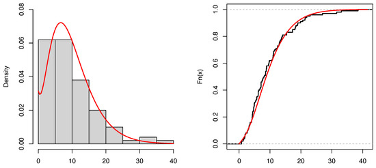
Figure 4. Plots of estimated pdf and CDF for the bank customers data.

Total Time on the Test (TTT) plot plays a vital role in selecting the proper model for fitting the underlying data regarding the failure rates. This informs us of the altered forms of the model failure rate. If the plot has a straight line, then the given data have a constant failure rate. The failure rates will be decreased if it is convex and increased if this plot is concave. For the bathtub shape, the TTT plot decreases first and then increases. Whereas, if the TTT plot is concave first and then convex, the failure rates will have an inverted bathtub shape. The TTT and density plots for TPXG distribution for the bank customers’ data are given in Figure 5. The probability–probability (P-P) and quantile–quantile (Q-Q) plots for the TPXG model based on the real data are given in Figure 6. Figure 7 presents the box and Bee Swarm plots for these data.

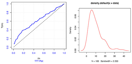
Figure 5. TTT and density plots for TPXG distribution for bank customer data.

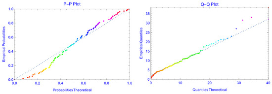
Figure 6. P-P and Q-Q plots for TPXG distribution for bank customers.

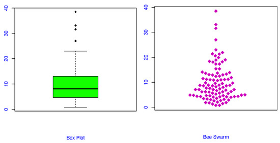
Figure 7. Box and Bee Swarm plots for TPXG distribution for bank customers.

Based on these data, we take an SRS of size 20, while for the ranked set sampling, a small sample size of $k=5$ is considered with number of cycles as $n=4$. Table 6 and Table 7 include the RSS (n = 4 and k = 5) and SRS ($N=20$) samples taken from the bank customers data. It is of interest to note here that the SRS and RSS methods are compared based on the same number of measured units. Using the previous methods, we calculate the estimates of $\beta$ and $\lambda$ in each design. Here, we assumed that the ranking is perfect. To compare estimators, we considered the previous criteria measures, AIC, BIC, CAIC HQC, and KS. The results are summarized in Table 8.

Table 6. RSS sample taken from the bank customers data for n = 4 and k = 5.

1st-Cycle:	1.9	8.9	7.4	15.4	38.5
2nd-Cycle:	2.1	1.9	8.6	7.4	13.3
3rd-Cycle:	4.8	6.3	8.9	17.3	18.2
4th-Cycle:	0.8	8.6	15.4	18.9	11.0

Table 7. SRS sample taken form the data set of size 20.

21.9	2.9	4.3	7.1	21.3	6.2	4.2	2.7	12.5	17.3
18.4	6.1	38.5	11.1	31.6	15.4	33.1	7.6	1.5	13.9

Table 8. Estimates, AIC, BIC, CAIC HQC, and KS in SRS and RSS design using MLE, MPS, OLS, WLS, CV, and AD.

Method	Design	AIC	BIC	AICS	HQC	KS
MLE	SRS	673.043	678.253	673.167	675.152	0.223
	RSS	648.315	653.526	648.439	650.424	0.102
MPS	SRS	680.050	685.261	680.174	682.159	0.228
	RSS	656.563	661.773	656.686	658.671	0.125
OLS	SRS	678.286	683.496	678.409	680.394	0.226
	RSS	650.269	655.479	650.393	652.378	0.098
WLS	SRS	678.174	683.384	678.298	680.283	0.235
	RSS	649.969	655.179	650.092	652.077	0.095
CV	SRS	672.151	677.362	672.275	674.260	0.226
	RSS	647.083	652.293	647.207	649.192	0.096
AD	SRS	674.156	679.366	674.280	676.265	0.228
	RSS	648.987	654.198	649.111	651.096	0.097

The findings in Table 8 illustrate that the TPXG parameter estimates, based on the RSS method, are improved compared to their counterparts in SRS in terms of the smallest values of AIC, BIC, CAIC HQC, and KS, using the MLE, MPS, OLS, WLS, CV, and AD.

5. Conclusions

This paper discusses several estimation methods for the TPXG distribution parameters based on RSS and SRS designs. A simulation study is performed to compare the performance of these various estimators, considering the same number of measuring units. A real data set is analyzed to illustrate the usefulness of the suggested estimators. Based on the obtained results, the RSS estimators are better than the SRS estimators in terms of MSE, bias, and efficiency values for all estimation methods considered in the paper. For future work, the topics discussed in this paper can be considered under imperfect ranking (Dell and Clutter [4]) based on RSS or using some of its modifications. For some modifications of the RSS, see the balanced groups RSS by Jemain et al. [30], percentile DRSS by Al-Omari and Jaber [31], and new mixed RSS by Hanandeh et al. [32]. Furthermore, one can use other real data sets for additional investigation of the suggested estimators of the TPXG distribution.

References

- Sen, S.; Maiti, S.S.; Chandra, N. The xgamma distribution: Statistical properties and application. J. Mod. Appl. Stat. Methods 2016, 15, 38. [Google Scholar] [CrossRef]
- McIntyre, G.A. A method for unbiased selective sampling using ranked set sampling. Aust. J. Agric. Res. 1952, 3, 385–390. [Google Scholar] [CrossRef]
- Takahasi, K.; Wakimoto, K. On unbiased estimates of the population mean based on the sample stratified by means of ordering. Ann. Inst. Stat. Math. 1968, 20, 1–31. [Google Scholar] [CrossRef]
- Dell, T.R.; Clutter, J.L. Ranked set sampling theory with order statistics background. Biometrics 1972, 28, 545–555. [Google Scholar] [CrossRef]
- Samawi, H.; Abu-Daayeh, H.A.; Ahmed, S. Estimating the population mean using extreme ranked set sampling. Biom. J. 1996, 38, 577–586. [Google Scholar] [CrossRef]
- Mutllak, H.A. Median ranked set sampling. J. Appl. Stat. Sci. 1997, 6, 245–255. [Google Scholar]
- Al-Saleh, M.F.; Al-Kadiri, M.A. Double-ranked set sampling. Stat. Probab. Lett. 2000, 48, 205–212. [Google Scholar] [CrossRef]
- Muttlak, H.A. Modified ranked set sampling methods. Pak. J. Stat.-All Ser. 2003, 19, 315–324. [Google Scholar] [CrossRef]
- Al-Nasser, A.D. L-Ranked set sampling: A generalization procedure for robust visual sampling. Commun. Stat. 2007, 6, 33–43. [Google Scholar] [CrossRef]
- Haq, A.; Brown, J.; Moltchanova, E.; Al-Omari, A.I. Partial ranked set sampling design. Environmetrics 2013, 24, 201–207. [Google Scholar] [CrossRef]
- Zamanzade, E.; Al-Omari, A.I. New ranked set sampling for estimating the population mean and variance. Hacet. J. Math. Stat. 2016, 45, 1891–1905. [Google Scholar] [CrossRef]
- Abu-Dayyeh, W.A.; Al-Subh, S.A.; Muttlak, H.A. Logistic parameters estimation using simple random sampling and ranked set sampling data. Appl. Math. Comput. 2004, 150, 543–554. [Google Scholar] [CrossRef]
- Al-Omari, A.I.; Benchiha, S.; Almanjahie, I.M. Efficient Estimation of the Generalized Quasi-Lindley Distribution Parameters under Ranked Set Sampling and Applications. Math. Probl. Eng. 2021, 1, 9982397. [Google Scholar] [CrossRef]
- Yousef, O.M.; Al-Subh, S.A. Estimation of Gumbel parameters under ranked set sampling. J. Mod. Appl. Stat. Methods 2014, 13, 24. [Google Scholar] [CrossRef]
- Akgul, F.G.; Şenoglu, B. Estimation of P (X< Y) using ranked set sampling for the Weibull distribution. Qual. Technol. Quant. Manag. 2017, 14, 296–309. [Google Scholar]
- Hussian, M.A. Bayesian and maximum likelihood estimation for Kumaraswamy distribution based on ranked set sampling. Am. J. Math. Stat. 2014, 4, 30–37. [Google Scholar]
- Chen, W.; Xie, M.; Wu, M. Parametric estimation for the scale parameter for scale distributions using moving extremes ranked set sampling. Stat. Probab. Lett. 2013, 83, 2060–2066. [Google Scholar] [CrossRef]
- Al-Omari, A.I.; Bouza, C.N. Ratio estimators of the population mean with missing values using ranked set sampling. Environmetrics 2015, 26, 67–76. [Google Scholar] [CrossRef]
- Al-Omari, A.I. Maximum likelihood estimation in location-scale families using varied L ranked set sampling. RAIRO-Oper. Res. 2021, 55, S2759–S2771. [Google Scholar] [CrossRef]
- Hassan, A.S.; Al-Omari, A.I.; Nagy, H.F. The Determination of the order of an autoregression. Iran. J. Sci. Technol. Trans. Sci. 2021, 45, 641–659. [Google Scholar] [CrossRef]
- Cheng, R.C.H.; Amin, N.A.K. Maximum product-of-spacings estimation with applications to the log-Normal distribution; Technical Report; Department of Mathematics, University of Wales: Cardiff, UK, 1979. [Google Scholar]
- Cheng, R.C.H.; Amin, N.A.K. Estimating parameters in continuous univariate distributions with a shifted origin. J. R. Stat. Soc. Ser. 1983, 45, 394–403. [Google Scholar] [CrossRef]
- Swain, J.; Venkatraman, S.; Wilson, J. Least squares estimation of distribution function in Johnson’s translation system. J. Stat. Comput. Simul. 1988, 29, 271–297. [Google Scholar] [CrossRef]
- D’Agostino, R.B.; Stephens, M.A. Goodness-of-Fit Techniques; Marcel Dekker: New York, NY, USA, 1986. [Google Scholar]
- Ghitany, M.E.; Atieh, B.; Nadarajah, S. Lindley distribution and its application. Math. Comput. Simul. 2008, 78, 493–506. [Google Scholar] [CrossRef]
- Akaike, H. A new look at the statistical model identification. IEEE Trans. Autom. Control 1974, 19, 716–723. [Google Scholar] [CrossRef]
- Schwarz, G. Estimating the dimension of a model. Ann. Stat. 1978, 6, 461–464. [Google Scholar] [CrossRef]
- Hannan, E.J.; Quinn, B.G. The Determination of the order of an autoregression. J. R. Stat. Soc. Ser. B 1979, 41, 190–195. [Google Scholar] [CrossRef]
- Bozdogan, H. Model selection and Akaike’s information criterion (AIC): The general theory and its analytical extensions. Psychometrika 1987, 52, 345–370. [Google Scholar] [CrossRef]
- Jemain, A.A.; Al-Omari, A.I.; Ibrahim, K. Balanced groups ranked set sampling for estimating the population median. J. Appl. Stat. 2008, 17, 39–46. [Google Scholar]
- Al-Omari, A.I.; Jaber, K. Percentile double ranked set sampling. J. Math. Stat. 2008, 4, 60–64. [Google Scholar] [CrossRef][Green Version]
- Hanandeh, A.A.; Al-Nasser, A.D.; Al-Omari, A.I. New mixed ranked set sampling variations. Stat 2022, 11, e417. [Google Scholar] [CrossRef]
Publisher’s Note: MDPI stays neutral with regard to jurisdictional claims in published maps and institutional affiliations. |
© 2022 by the authors. Licensee MDPI, Basel, Switzerland. This article is an open access article distributed under the terms and conditions of the Creative Commons Attribution (CC BY) license (https://creativecommons.org/licenses/by/4.0/).