Some Asymptotic Properties of a Kernel Bispectum Estimate with Different Multitapers

Abstract

Assume $X_1,X_2,\dots ,X_N$ are realizations of N observations from a real-valued discrete parameter third-order stationary process $X_t,t=0\pm 1,\pm 2,\dots$, with bispectrum $f_{XXX}({\lambda }_1,{\lambda }_2)$ where “$-\pi \le {\lambda }_1,{\lambda }_2\le \pi$”. Based on the previous assumption, L different multitapered biperiodograms $I_{XXX}^{{\left(mt\right)}_j}({\lambda }_1,{\lambda }_2);j=1,2,\dots ,L$ on overlapped segments ($X_t^{\left(j\right)};1\le t<N$) can be constructed. Further, the mean and variance of the average of these different multitapered biperiodograms can be expressed as asymptotic expressions. According to different bispectral windows/kernels ($W_{\beta }^{\left(j\right)}({\alpha }_1,{\alpha }_2)$, where “$-\pi ⩽{\alpha }_1,{\alpha }_2⩽\pi$” and$\beta$ is the bandwidth) and $I_{XXX}^{{\left(mt\right)}_j}({\lambda }_1,{\lambda }_2)$, the bispectrum $f_{XXX}({\lambda }_1,{\lambda }_2)$ can be estimated. The asymptotic expressions of the first- and second-ordered moments as well as the integrated relative mean squared error (IMSE) of this estimate are derived. Finally, some estimation results based on numerically generated data from the selected process “DCGINAR(1)” are presented and discussed in detail.

1. Introduction

The multitapering approach has been widely applied in the geophysical field. Furthermore, it has been demonstrated in numerous instances to perform better than the single-tapered smoothed periodogram (see [1,2,3]). The performance advantage of the multitapering technique is quantified relative to overlapped segments. This is due to the method’s ability to produce estimates with lower levels of variance while preserving the good bias features provided by tapers (see [4,5]). Several authors used tapered data to study some asymptotic statistical characteristics of spectral estimates (see [6,7,8]). At the IEEE workshop on higher-order statistics, ref. [9] studied the statistical properties of multi-window bispectrum estimates. Ref. [10] discussed properties of multitaper estimators for both power and bispectral density functions. Ref. [11] demonstrated a unified view of multitaper multivariate spectral estimation. Ref. [12] developed a multiple window bispectrum estimator (MWBE), which was derived from the best tapers with the largest concentration of bifrequency and has strong variance features. Through the use of various tapers and weight functions (kernels), the asymptotic formulations of the first- and second-order moments of specific spectral estimates on overlapped segments for stationary processes in both continuous and discrete time were studied in [13,14]. Ref. [15] discussed an approach for using the multitapering technique to evaluate a multidimensional strictly stationary time series with some arbitrarily distorted data in the frequency domain. By Thomson’s modified approach, ref. [16] produced an enhanced multitaper spectral estimate to reduce for curvature bias. Ref. [17] study the problem of estimating a spectral density function (spectrum) using different multitapers for a discrete parameter stationary time series. Ref. [18] introduced an R package that uses sine multitapers and allows the number to vary with frequency to lower mean square error in order to compute univariate power spectral density estimates with little to no tuning effort. Ref. [19] presented a review of multitaper spectral analysis. Ref. [20] presented a spectral analysis of wave elevation time histories using the multitaper method. Ref. [21] presented a spectral estimator by explicitly modelling the spectral dynamics by fusing the multitaper approach with state-space models in a Bayesian estimating framework. Ref. [22] addressed these shortcomings by explicitly modeling the spectral dynamics through integrating the multitaper method with state-space models in a Bayesian estimation framework. Ref. [23] addressed the multitaper spectral analysis of latent stationary processes that generate neural spiking activity. Ref. [24] improved the convergence of spectral proper orthogonal decomposition using multitaper estimates. Ref. [25] used the adaptive multitaper approach, a nonparametric spectrum analysis method appropriate for time series with coloured power spectral density, to analyse the power spectral density. The multitaper S-transform (MTST) approach was developed by [26] to estimate the evolutionary power spectral density (EPSD) and coherence of multivariate non-stationary processes. There are many previous studies that estimated the spectral density function in case of overlapping segments. However, the situation is more complicated in case of bispectral density functions.

The main aim of this paper is that, due to the difficulty of finding a bispectral density function estimator in the case of overlapping segments for a discrete parameter stationary time series, a novel bispectral density function estimator is proposed and discussed in detail. The new estimator depends on various multitapers. Thus, the bispectral density function is estimated utilizing the average of its estimators across all segments, and the Bartlett window (kernel) is applied to smooth this estimator. Consequently the resulting estimator is called a smoothed multitapering biperiodogram. Some statistical and approximate properties of the introduced estimator are derived. Not being able to find natural observations, a smoothed multitapering biperiodogram is reported as an estimator of the bispectral density function based on a well-known process called DCGINAR(1) (see [27] and Theorem 6 in [28]). Finally, a simulation is utilized to obtain the best smoothed multitapering biperiodogram.

The structure of this paper is as follows: Section 2 introduces a bispectral density function estimate utilising various multitapers and bispctral windows (kernels). The asymptotic equations for the mean and variance of the average of the different multitapered biperiodograms that were constructed are expressed. In Section 3, under the assumption that the multitapered bispectral estimates are uncorrelated, the asymptotic expressions of the mean and variance for the proposed estimate are obtained. In addition, by analysing the bias and variance of this estimate, we are able to suggest a certain bandwidth. The integrated relative mean squared error of the estimate is also expressed asymptotically in our work. In Section 4, the numerical results for the proposed estimator for the dependent counting geometric INAR(1) (DCGINAR(1)) process are shown. Section 5 concludes the paper by providing a summary.

2. The Structural Model

Assume $X_1,X_2,\dots ,X_N$ are realizations of N observations from a real-valued discrete parameter third-order stationary process $X_t,t=0\pm 1,\pm 2,\dots$, with $\mu =E\left(X_t\right)$. The bispectral density function of $X_t$ is

$$f_{XXX}({\lambda }_1,{\lambda }_2)=\frac{1}{{\left(2\pi \right)}^2}\sum _{t_1=-\infty }^{\infty }\sum _{t_2=-\infty }^{\infty }{C}_{XXX}(t_1,t_2)e^{-i{t}_1{\lambda }_1-i{t}_2{\lambda }_2},-\pi \le {\lambda }_1,{\lambda }_2\le \pi ,$$

(1)

where $C_{XXX}(t_1,t_2)$ is the third-order covariance function of $X_t$ and given by

$$C_{XXX}(t_1,t_2)=E\left[(X_t-\mu )(X_{t+t_1}-\mu )(X_{t+t_2}-\mu )\right],$$

(2)

provided that ${\sum }_{t_1=-\infty }^{\infty }{\sum }_{t_2=-\infty }^{\infty }\mid C_{XXX}(t_1,t_2)\mid <\infty$. If the process $X_t$ is invertible, then the inverse bispectral density function is defined by

$$f_{XXX}^{-1}({\lambda }_1,{\lambda }_2)=\frac{1}{{\left(2\pi \right)}^2}\sum _{t_1=-\infty }^{\infty }\sum _{t_2=-\infty }^{\infty }{d}_{XXX}(t_1,t_2)e^{-i{t}_1{\lambda }_1-i{t}_2{\lambda }_2},$$

(3)

such that ${\sum }_{t_1=-\infty }^{\infty }{\sum }_{t_2=-\infty }^{\infty }\mid d_{XXX}(t_1,t_2)\mid <\infty$, where $d_{XXX}(t_1,t_2)$ is the inverse third-order covariance of $X_t$. We construct L segments by dividing the given observations:

$$X_t^{\left(j\right)}=X_{\left[\right(j-1)n+t]},j=1,2,\dots ,L;t=1,2,\dots ,n+q;0\le q<n,$$

(4)

where $X_t^{\left(j\right)}$ is the set of observations in the $j^{th}$ segment. If $N=Ln+q;0<q<n$, then the number of overlapped segments $L=(N-q)/n$ and each segment contains $n+q$ observations. Additionally, if $q=0$, then the number of non-overlapped segments $L=N/n$. Now, we define the average of different multitapered biperiodograms as an estimate of $f_{XXX}({\lambda }_1,{\lambda }_2)$

$${\widehat{f}}_{XXX}^{\left(mt\right)}({\lambda }_1,{\lambda }_2)=\frac{1}{L}\sum _{j=1}^L{I}_{XXX}^{{\left(mt\right)}_j}({\lambda }_1,{\lambda }_2),$$

(5)

where $I_{XXX}^{{\left(mt\right)}_j}({\lambda }_1,{\lambda }_2)$ is the multitapered biperiodogram of $X^{\left(j\right)}\left(t\right)$ given by (see [9,12])

$$\begin{array}{c}\hfill I_{XXX}^{{\left(mt\right)}_j}({\lambda }_1,{\lambda }_2)=\frac{1}{{\left(2\pi \right)}^2\gamma }\sum _{k=1}^K\sum _{l=1}^K\sum _{m=1}^{K}Q(k,l,m)[\sum _{t=1}^{n+q}{h}_k\left(t\right)X_t^{\left(j\right)}{e}^{-i{\lambda }_{1}t}]\\ \hfill \times [\sum _{t=1}^{n+q}{h}_l\left(t\right)X_t^{\left(j\right)}{e}^{-i{\lambda }_{2}t}[[\sum _{t=1}^{n+q}{h}_m\left(t\right)X_t^{\left(j\right)}{e}^{i({\lambda }_1+{\lambda }_2)t}],\end{array}$$

(6)

where the three-dimensional weight function is

$$Q(k,l,m)=\sum _{t=1}^{n+q}{h}_k\left(t\right)h_l\left(t\right)h_m\left(t\right),$$

(7)

and the normalizing constant $\gamma$ is defined by

$$\gamma =\sum _{k=1}^K\sum _{l=1}^K\sum _{m=1}^K{Q}^2(k,l,m),$$

(8)

where K is the number of tapers applied in the averaging, $h_k\left(t\right),h_l\left(t\right)$ and $h_m\left(t\right)$ are data tapers or lag windows and equal to zero outside the interval $[1,n+q]$, the time index is $t=1,\dots ,n+q$, and the subscripts $k,l,m=0,1,\dots ,K$ denote the window order. In this paper, three lag windows are used. These lag windows are the Parzen window, Daniell window and Tukey–Hamming window. Ref. [29] introduced the Parzen lag window

$$h\left(t\right)=\left\{\begin{array}{cc}1-6{\left(\frac{t}{M}\right)}^2+6{\left(\frac{\left|t\right|}{M}\right)}^3;\hfill & \left|t\right|\le \frac{M}{2}\hfill \\ 2{(1-\frac{\left|t\right|}{M})}^3;\hfill & \frac{M}{2}<\left|t\right|\le M\hfill \\ 0;\hfill & \left|t\right|>M,\hfill \end{array}\right.$$

(9)

Ref. [30] introduced the Daniell lag window as

$$h\left(t\right)=\frac{sin\left(\frac{t\pi }{M}\right)}{\frac{t\pi }{M}},$$

(10)

and [31] proposed the Tukey–Hamming window as

$$h\left(t\right)=\left\{\begin{array}{cc}0.5+0.5cos\left(\frac{t\pi }{M}\right);\hfill & \left|t\right|\le M\hfill \\ 0;\hfill & \left|t\right|>M,\hfill \end{array}\right.$$

(11)

where M is some integer less than $(N-1)$ whose precise value is as yet unspecified, and sometimes called the window parameter or number of frequencies used in smoothing. In fact, the multitapered biperiodogram $I_{XXX}^{\left(mt\right)}({\lambda }_1,{\lambda }_2)$ has the asymptotic properties (see [9,12])

$$\begin{array}{cc}\hfill & E\left[I_{XXX}^{\left(mt\right)}({\lambda }_1,{\lambda }_2)\right]\approx f_{XXX}({\lambda }_1,{\lambda }_2),\hfill \\ \hfill Var\left[I_{XXX}^{\left(mt\right)}({\lambda }_1,{\lambda }_2)\right]& \approx \frac{1}{3w^2(n+q)}{f}_{XX}\left({\lambda }_1\right)f_{XX}\left({\lambda }_2\right)f_{XX}({\lambda }_1+{\lambda }_2),\hfill \end{array}$$

(12)

where $f_{XX}(.)$ is the power spectral density function of $X_t$ and w is fixed ( $0<w<\frac{1}{2}$). By using (5), (12) and the uncorrelation of multitapered $I_{XXX}^{{\left(mt\right)}_j}({\lambda }_1,{\lambda }_2)$ biperiodogram, then

$$\begin{array}{cc}\hfill & E\left[f_{XXX}^{\left(mt\right)}({\lambda }_1,{\lambda }_2)\right]\approx f_{XXX}({\lambda }_1,{\lambda }_2),\hfill \\ \hfill Var\left[f_{XXX}^{\left(mt\right)}({\lambda }_1,{\lambda }_2)\right]& \approx \frac{1}{3w^2(n+q)L}{f}_{XX}\left({\lambda }_1\right)f_{XX}\left({\lambda }_2\right)f_{XX}({\lambda }_1+{\lambda }_2).\hfill \end{array}$$

Smoothing the multitapered biperiodograms $I_{XXX}^{{\left(mt\right)}_j}({\lambda }_1,{\lambda }_2),j=1,2,\dots ,L$ by the kernel (bispectral window) $W_{\beta }^{\left(j\right)}({\alpha }_1,{\alpha }_2),-\pi ⩽{\alpha }_1,{\alpha }_2⩽\pi$ (see [32]), we obtain

$${\widehat{f}}_{XXX}^{{\left(mt\right)}_{sp}}({\lambda }_1,{\lambda }_2)=\frac{1}{{\beta }^{2}L}\sum _{j=1}^L\underset{-\pi }{\overset{\pi }{\int }}\underset{-\pi }{\overset{\pi }{\int }}{W}^{\left(j\right)}(\frac{{\lambda }_1-\mu }{\beta },\frac{{\lambda }_2-\nu }{\beta })I_{XXX}^{{\left(mt\right)}_j}(\mu ,\nu )d\mu d\nu ,$$

(13)

which is a smoothed estimate of $f_{XXX}({\lambda }_1,{\lambda }_2)$ with $W_{\beta }^{\left(j\right)}({\alpha }_1,{\alpha }_2)=\frac{1}{{\beta }^2}W(\frac{{\alpha }_1}{\beta },\frac{{\alpha }_2}{\beta })$, such that ${\int }_{-\pi }^{\pi }{\int }_{-\pi }^{\pi }{W}^{\left(j\right)}({\alpha }_1,{\alpha }_2)d{\alpha }_{1}d{\alpha }_2=1,W^{\left(j\right)}({\alpha }_1,{\alpha }_2)=W^{\left(j\right)}({\alpha }_2,{\alpha }_1)=W^{\left(j\right)}({\alpha }_1,-{\alpha }_1-{\alpha }_2)=W^{\left(j\right)}(-{\alpha }_1-{\alpha }_2,-{\alpha }_2).$ $\beta$ is called the bandwidth (see [32]). The bispectral window $W^{\left(j\right)}({\alpha }_1,{\alpha }_2)$ can be derived from spectral windows as (see [33])

$$W^{\left(j\right)}({\alpha }_1,{\alpha }_2)=W^{\left(j\right)}\left({\alpha }_1\right)W^{\left(j\right)}\left({\alpha }_2\right)W^{\left(j\right)}({\alpha }_1+{\alpha }_2).$$

In this paper, we use the Bartlett spectral window (see [34]), which is given by

$$W^{\left(j\right)}\left(\alpha \right)=\frac{1}{2\pi }{\left[\frac{sin\left(\frac{\alpha }{2}\right)}{\frac{\alpha }{2}}\right]}^2.$$

(14)

We can deduce (13) to

$${\widehat{f}}_{XXX}^{{\left(mt\right)}_{sp}}({\lambda }_1,{\lambda }_2)=\frac{1}{L}\sum _{j=1}^L{\widehat{f}}_{XXX}^{{\left(mt\right)}_j}({\lambda }_1,{\lambda }_2),$$

(15)

where

$${\widehat{f}}_{XXX}^{{\left(mt\right)}_j}({\lambda }_1,{\lambda }_2)=\frac{1}{{\beta }^2}\underset{-\pi }{\overset{\pi }{\int }}\underset{-\pi }{\overset{\pi }{\int }}{W}^{\left(j\right)}(\frac{{\lambda }_1-\mu }{\beta },\frac{{\lambda }_2-\nu }{\beta })I_{XXX}^{{\left(mt\right)}_j}(\mu ,\nu )d\mu d\nu ,$$

(16)

is the $j^{th}$ smoothed multitapered biperiodogram of $X^{\left(j\right)}\left(t\right)$.

3. Statistical Properties of ${\widehat{\mathit{f}}}_{\mathit{XXX}}^{{\left(\mathit{mt}\right)}_{\mathit{sp}}}({\mathit{\lambda }}_{\mathit{1}},{\mathit{\lambda }}_{\mathit{2}})$

The asymptotic equations of the expectation, variance, and IMSE of the smoothed (kernel) bispectrum estimator ${\widehat{f}}_{XXX}^{{\left(mt\right)}_{sp}}({\lambda }_1,{\lambda }_2)$ are given in this section.

3.1. Expected Value

Taking the expectation of (13), then

$$E\left[{\widehat{f}}_{XXX}^{{\left(mt\right)}_{sp}}({\lambda }_1,{\lambda }_2)\right]\approx \frac{1}{{\beta }^{2}L}\sum _{j=1}^L\underset{-\pi }{\overset{\pi }{\int }}\underset{-\pi }{\overset{\pi }{\int }}{W}^{\left(j\right)}(\frac{{\lambda }_1-\mu }{\beta },\frac{{\lambda }_2-\nu }{\beta })f_{XXX}(\mu ,\nu )d\mu d\nu .$$

(17)

Making the transformation by taking $\mu ={\lambda }_1-\beta {\alpha }_1,\nu ={\lambda }_2-\beta {\alpha }_2$, with small $\beta ;{\lambda }_1,{\lambda }_2\in (-\pi ,\pi ]$, then (17) becomes

$$E\left[{\widehat{f}}_{XXX}^{{\left(mt\right)}_{sp}}({\lambda }_1,{\lambda }_2)\right]\approx \frac{1}{L}\sum _{j=1}^L\underset{-\infty }{\overset{\infty }{\int }}\underset{-\infty }{\overset{\infty }{\int }}{W}^{\left(j\right)}({\alpha }_1,{\alpha }_2)f_{XXX}({\lambda }_1-\beta {\alpha }_1,{\lambda }_2-\beta {\alpha }_2)d{\alpha }_{1}d{\alpha }_2,$$

(18)

by using the Taylor expansion for $f_{XXX}({\lambda }_1-\beta {\alpha }_1,{\lambda }_2-\beta {\alpha }_2)$ about ${\lambda }_1$ and ${\lambda }_2$, we can write (18) as

$$\begin{array}{cc}\hfill E[{\widehat{f}}_{XXX}^{{\left(mt\right)}_{sp}}& ({\lambda }_1,{\lambda }_2)]=\frac{1}{L}\sum _{j=1}^L\underset{-\infty }{\overset{\infty }{\int }}\underset{-\infty }{\overset{\infty }{\int }}{W}^{\left(j\right)}({\alpha }_1,{\alpha }_2)[f_{XXX}({\lambda }_1,{\lambda }_2)-\beta {\alpha }_1\frac{\partial f_{XXX}({\lambda }_1,{\lambda }_2)}{\partial {\lambda }_1}\hfill \\ \hfill & -\beta {\alpha }_2\frac{\partial f_{XXX}({\lambda }_1,{\lambda }_2)}{\partial {\lambda }_2}+\frac{1}{2!}(\frac{{\beta }^2{\alpha }_1^2{\partial }^2{f}_{XXX}({\lambda }_1,{\lambda }_2)}{\partial {\lambda }_1^2}+\frac{2{\alpha }_1{\alpha }_2{\beta }^2{\partial }^2{f}_{XXX}({\lambda }_1,{\lambda }_2)}{\partial {\lambda }_1\partial {\lambda }_2}\hfill \\ \hfill & +\frac{{\beta }^2{\alpha }_2^2{\partial }^2{f}_{XXX}({\lambda }_1,{\lambda }_2)}{\partial {\lambda }_2^2}+o\left({\beta }^2\right)\left)\right]d{\alpha }_{1}d{\alpha }_2.\hfill \end{array}$$

(19)

$$\begin{array}{cc}\hfill E\left[{\widehat{f}}_{XXX}^{{\left(mt\right)}_{sp}}({\lambda }_1,{\lambda }_2)\right]=& f_{XXX}({\lambda }_1,{\lambda }_2)-\frac{\beta }{L}\frac{\partial f_{XXX}({\lambda }_1,{\lambda }_2)}{\partial {\lambda }_1}\sum _{j=1}^L\underset{-\infty }{\overset{\infty }{\int }}\underset{-\infty }{\overset{\infty }{\int }}{\alpha }_1{W}^{\left(j\right)}({\alpha }_1,{\alpha }_2)d{\alpha }_{1}d{\alpha }_2\hfill \\ \hfill & -\frac{\beta }{L}\frac{\partial f_{XXX}({\lambda }_1,{\lambda }_2)}{\partial {\lambda }_2}\sum _{j=1}^L\underset{-\infty }{\overset{\infty }{\int }}\underset{-\infty }{\overset{\infty }{\int }}{\alpha }_2{W}^{\left(j\right)}({\alpha }_1,{\alpha }_2)d{\alpha }_{1}d{\alpha }_2\hfill \\ \hfill & +\frac{{\beta }^2}{2!L}\frac{{\partial }^2{f}_{XXX}({\lambda }_1,{\lambda }_2)}{\partial {\lambda }_1^2}\sum _{j=1}^L\underset{-\infty }{\overset{\infty }{\int }}\underset{-\infty }{\overset{\infty }{\int }}{\alpha }_1^2{W}^{\left(j\right)}({\alpha }_1,{\alpha }_2)d{\alpha }_{1}d{\alpha }_2\hfill \\ & +\frac{2{\beta }^2}{2!L}\frac{{\partial }^2{f}_{XXX}({\lambda }_1,{\lambda }_2)}{\partial {\lambda }_1\partial {\lambda }_2}\sum _{j=1}^L\underset{-\infty }{\overset{\infty }{\int }}\underset{-\infty }{\overset{\infty }{\int }}{\alpha }_1{\alpha }_2{W}^{\left(j\right)}({\alpha }_1,{\alpha }_2)d{\alpha }_{1}d{\alpha }_2\hfill \\ \hfill & +\frac{{\beta }^2}{2!L}\frac{{\partial }^2{f}_{XXX}({\lambda }_1,{\lambda }_2)}{\partial {\lambda }_2^2}\sum _{j=1}^L\underset{-\infty }{\overset{\infty }{\int }}\underset{-\infty }{\overset{\infty }{\int }}{\alpha }_2^2{W}^{\left(j\right)}({\alpha }_1,{\alpha }_2)d{\alpha }_{1}d{\alpha }_2+o\left({\beta }^2\right),\hfill \end{array}$$

(20)

since $\underset{-\infty }{\overset{\infty }{\int }}\underset{-\infty }{\overset{\infty }{\int }}{\alpha }_i{W}^{\left(j\right)}({\alpha }_1,{\alpha }_2)d{\alpha }_{1}d{\alpha }_2=0\forall i=1,2$ (see [32]), then

$$\begin{array}{cc}\hfill E\left[{\widehat{f}}_{XXX}^{{\left(mt\right)}_{sp}}({\lambda }_1,{\lambda }_2)\right]=& f_{XXX}({\lambda }_1,{\lambda }_2)+\frac{{\beta }^2}{2L}\frac{{\partial }^2{f}_{XXX}({\lambda }_1,{\lambda }_2)}{\partial {\lambda }_1^2}\sum _{j=1}^L\underset{-\infty }{\overset{\infty }{\int }}\underset{-\infty }{\overset{\infty }{\int }}{\alpha }_1^2{W}^{\left(j\right)}({\alpha }_1,{\alpha }_2)d{\alpha }_{1}d{\alpha }_2\hfill \\ & +\frac{{\beta }^2}{L}\frac{{\partial }^2{f}_{XXX}({\lambda }_1,{\lambda }_2)}{\partial {\lambda }_1\partial {\lambda }_2}\sum _{j=1}^L\underset{-\infty }{\overset{\infty }{\int }}\underset{-\infty }{\overset{\infty }{\int }}{\alpha }_1{\alpha }_2{W}^{\left(j\right)}({\alpha }_1,{\alpha }_2)d{\alpha }_{1}d{\alpha }_2\hfill \\ \hfill & +\frac{{\beta }^2}{2L}\frac{{\partial }^2{f}_{XXX}({\lambda }_1,{\lambda }_2)}{\partial {\lambda }_2^2}\sum _{j=1}^L\underset{-\infty }{\overset{\infty }{\int }}\underset{-\infty }{\overset{\infty }{\int }}{\alpha }_2^2{W}^{\left(j\right)}({\alpha }_1,{\alpha }_2)d{\alpha }_{1}d{\alpha }_2+o\left({\beta }^2\right).\hfill \end{array}$$

(21)

Accordingly, the bias of ${\widehat{f}}_{XXX}^{{\left(mt\right)}_{sp}}({\lambda }_1,{\lambda }_2)$ can be formulated as

$$\begin{array}{cc}\hfill Bias[{\widehat{f}}_{XXX}^{{\left(mt\right)}_{sp}}(& {\lambda }_1,{\lambda }_2\left)\right]\approx \frac{{\beta }^2}{2L}\frac{{\partial }^2{f}_{XXX}({\lambda }_1,{\lambda }_2)}{\partial {\lambda }_1^2}\sum _{j=1}^L\underset{-\infty }{\overset{\infty }{\int }}\underset{-\infty }{\overset{\infty }{\int }}{\alpha }_1^2{W}^{\left(j\right)}({\alpha }_1,{\alpha }_2)d{\alpha }_{1}d{\alpha }_2\hfill \\ & +\frac{{\beta }^2}{L}\frac{{\partial }^2{f}_{XXXX}({\lambda }_1,{\lambda }_2)}{\partial {\lambda }_1\partial {\lambda }_2}\sum _{j=1}^L\underset{-\infty }{\overset{\infty }{\int }}\underset{-\infty }{\overset{\infty }{\int }}{\alpha }_1{\alpha }_2{W}^{\left(j\right)}({\alpha }_1,{\alpha }_2)d{\alpha }_{1}d{\alpha }_2\hfill \\ \hfill & +\frac{{\beta }^2}{2L}\frac{{\partial }^2{f}_{XXX}({\lambda }_1,{\lambda }_2)}{\partial {\lambda }_2^2}\sum _{j=1}^L\underset{-\infty }{\overset{\infty }{\int }}\underset{-\infty }{\overset{\infty }{\int }}{\alpha }_2^2{W}^{\left(j\right)}({\alpha }_1,{\alpha }_2)d{\alpha }_{1}d{\alpha }_2.\hfill \end{array}$$

(22)

Note that the bias of ${\widehat{f}}_{XXX}^{{\left(mt\right)}_{sp}}({\lambda }_1,{\lambda }_2)$ is the order of $\left({\beta }^2{L}^{-1}\right)$.

3.2. Variance

Since the multitapered biperiodogram ordinates ${\widehat{f}}_{XXX}^{{\left(mt\right)}_j}({\mu }_a,{\nu }_b),1⩽a,b<(n+q)/2,$ are asymptotically independent (see [35,36]), then (13) can be expressed as

$$\begin{array}{cc}\hfill {\widehat{f}}_{XXX}^{{\left(mt\right)}_{sp}}({\lambda }_1,{\lambda }_2)& =\frac{1}{{\beta }^{2}L}\sum _{j=1}^L\sum _a^{}\sum _b^{}\underset{{\mu }_{a-1}}{\overset{{\mu }_a}{\int }}\underset{{\nu }_{b-1}}{\overset{{\nu }_b}{\int }}{W}^{\left(j\right)}(\frac{{\lambda }_1-\mu }{\beta },\frac{{\lambda }_2-\nu }{\beta })I_{XXX}^{{\left(mt\right)}_j}(\mu ,\nu )d\mu d\nu \hfill \\ \hfill & \approx \frac{4{\pi }^2}{{\beta }^{2}L{(n+q)}^2}\sum _{j=1}^L\sum _a^{}\sum _b^{}{W}^{\left(j\right)}(\frac{{\lambda }_1-{\mu }_a}{\beta },\frac{{\lambda }_2-{\nu }_b}{\beta })I_{XXX}^{{\left(mt\right)}_j}({\mu }_a,{\nu }_b).\hfill \end{array}$$

From (28), we get

$$\begin{array}{cc}\hfill Var\left({\widehat{f}}_{XXX}^{{\left(mt\right)}_{sp}}({\lambda }_1,{\lambda }_2)\right)\approx & \frac{16{\pi }^4}{3{\beta }^4{w}^2{L}^2{(n+q)}^5}\sum _{j=1}^L\sum _a^{}\sum _b^{}{\left[W^{\left(j\right)}(\frac{{\lambda }_1-{\mu }_a}{\beta },\frac{{\lambda }_2-{\nu }_b}{\beta })\right]}^2\hfill \\ \hfill & \times f_{XX}\left({\mu }_a\right)f_{XX}\left({\nu }_b\right)f_{XX}({\mu }_a+{\nu }_b)\hfill \\ \hfill \approx & \frac{4{\pi }^2}{3{\beta }^4{w}^2{L}^2{(n+q)}^3}\sum _{j=1}^L\underset{-\pi }{\overset{\pi }{\int }}\underset{-\pi }{\overset{\pi }{\int }}{\left[W^{\left(j\right)}(\frac{{\lambda }_1-\mu }{\beta },\frac{{\lambda }_2-\nu }{\beta })\right]}^2\hfill \\ \hfill & \times f_{XX}\left(\mu \right)f_{XX}\left(\nu \right)f_{XX}(\mu +\nu )d\mu d\nu .\hfill \end{array}$$

Putting $\mu ={\lambda }_1-\beta {\alpha }_1$ and $\nu ={\lambda }_2-\beta {\alpha }_2$,

$$\begin{array}{cc}\hfill Var\left({\widehat{f}}_{XXX}^{{\left(mt\right)}_{sp}}({\lambda }_1,{\lambda }_2)\right)& =\frac{4{\pi }^2}{3{\beta }^2{w}^2{L}^2{(n+q)}^3}\sum _{j=1}^L\underset{-\infty }{\overset{\infty }{\int }}\underset{-\infty }{\overset{\infty }{\int }}{\left[W^{\left(j\right)}({\alpha }_1,{\alpha }_2)\right]}^2{f}_{XX}({\lambda }_1-\beta {\alpha }_1)\hfill \\ \hfill & \times f_{XX}({\lambda }_2-\beta {\alpha }_2)f_{XX}({\lambda }_1+{\lambda }_2-\beta {\alpha }_1-\beta {\alpha }_2)d{\alpha }_{1}d{\alpha }_2\hfill \\ \hfill & \approx \frac{4{\pi }^2}{3{\beta }^2{w}^2{L}^2{(n+q)}^3}{f}_{XX}\left({\lambda }_1\right)f_{XX}\left({\lambda }_2\right)f_{XX}({\lambda }_1+{\lambda }_2)\hfill \\ \hfill & \times \sum _{j=1}^L{\int }_{-\infty }^{\infty }{\int }_{-\infty }^{\infty }{\left[W^{\left(j\right)}({\alpha }_1,{\alpha }_2)\right]}^{2}d{\alpha }_{1}d{\alpha }_2,\hfill \end{array}$$

(23)

which is of the order ${\left[{\beta }^2{L}^2{(n+q)}^3\right]}^{-1}$. The mean squared errors $\left(MSEs\right)$ of ${\widehat{f}}_{XXX}^{{\left(mt\right)}_{sp}}({\lambda }_1,{\lambda }_2)$ are defined as

$$MSE\left({\widehat{f}}_{XXX}^{{\left(mt\right)}_{sp}}({\lambda }_1,{\lambda }_2)\right)={\left(Bias\left[{\widehat{f}}_{XXX}^{{\left(mt\right)}_{sp}}({\lambda }_1,{\lambda }_2)\right]\right)}^2+Var\left[{\widehat{f}}_{XXX}^{{\left(mt\right)}_{sp}}({\lambda }_1,{\lambda }_2)\right].$$

The bias term and variance term both need to be small for this $MSEs$ to be small. We demonstrated earlier that these terms are of the order ${\beta }^2{L}^{-1}$ and ${\left[{\beta }^2{L}^2{(n+q)}^3\right]}^{-1}$, respectively, in Equations (22) and (23). Therefore, the variance and the squared bias terms of ${\widehat{f}}_{XX}^{{\left(mt\right)}_{sp}}({\lambda }_1,{\lambda }_2)$ are matched for ${\left[{\beta }^2{L}^2{(n+q)}^3\right]}^{-1}\approx {\beta }^4{L}^{-2}$. It follows that the ideal bandwidth option is $\beta \approx {(n+q)}^{-\frac{1}{2}}$. Hence $\beta ⟶0$ as $n⟶\infty$. Depending on the optimal choice of $\beta$, we get from (22) and (23)

$$Bias\left[{\widehat{f}}_{XX}^{{\left(mt\right)}_{sp}}({\lambda }_1,{\lambda }_2)\right],Var\left[{\widehat{f}}_{XXX}^{{\left(mt\right)}_{sp}}({\lambda }_1,{\lambda }_2)\right]⟶0,n⟶\infty ,$$

(24)

that is, ${\widehat{f}}_{XXX}^{{\left(mt\right)}_{sp}}({\lambda }_1,{\lambda }_2)$ is a consistent estimate of $f_{XXX}({\lambda }_1,{\lambda }_2)$ as $n⟶\infty$. Additionally, $Var\left({\widehat{f}}_{XXX}^{{\left(mt\right)}_{sp}}({\lambda }_1,{\lambda }_2)\right)$ has less variability as n increases.

3.3. Integrated Relative Mean Squared Error

For spectral estimates, we use IMSE as a gauge of the goodness of fit (see [37]). The IMSE of ${\widehat{f}}_{XXX}^{{\left(mt\right)}_{sp}}({\lambda }_1,{\lambda }_2)$ is defined by

$$\begin{array}{c}IMSE\left[{\widehat{f}}_{XXX}^{{\left(mt\right)}_{sp}}({\lambda }_1,{\lambda }_2)\right]=\underset{-\pi }{\overset{\pi }{\int }}\underset{-\pi }{\overset{\pi }{\int }}E{\left[\frac{{\widehat{f}}_{XXX}^{{\left(mt\right)}_{sp}}({\lambda }_1,{\lambda }_2)-f_{XXX}({\lambda }_1,{\lambda }_2)}{f_{XXX}({\lambda }_1,{\lambda }_2)}\right]}^{2}d{\lambda }_{1}d{\lambda }_2\hfill \\ \hfill =\underset{-\pi }{\overset{\pi }{\int }}\underset{-\pi }{\overset{\pi }{\int }}{\left[\frac{E\left[{\widehat{f}}_{XXX}^{{\left(mt\right)}_{sp}}({\lambda }_1,{\lambda }_2)\right]}{f_{XXX}({\lambda }_1,{\lambda }_2)}-1\right]}^{2}d{\lambda }_{1}d{\lambda }_2+\underset{-\pi }{\overset{\pi }{\int }}\underset{-\pi }{\overset{\pi }{\int }}Var\left[\frac{{\widehat{f}}_{XXX}^{{\left(mt\right)}_{sp}}({\lambda }_1,{\lambda }_2)}{f_{XXX}({\lambda }_1,{\lambda }_2)}\right]d{\lambda }_{1}d{\lambda }_2.\end{array}$$

Hence,

$$\begin{array}{cc}\hfill & IMSE\left[{\widehat{f}}_{XXX}^{{\left(mt\right)}_{sp}}({\lambda }_1,{\lambda }_2)\right]=4{\pi }^2+\underset{-\pi }{\overset{\pi }{\int }}\underset{-\pi }{\overset{\pi }{\int }}{\left[f_{XXX}^{-1}({\lambda }_1,{\lambda }_2)\right]}^2{\left(E\left[{\widehat{f}}_{XXX}^{{\left(mt\right)}_{sp}}({\lambda }_1,{\lambda }_2)\right]\right)}^{2}d{\lambda }_{1}d{\lambda }_2\hfill \\ \hfill & -2\underset{-\pi }{\overset{\pi }{\int }}\underset{-\pi }{\overset{\pi }{\int }}{f}_{XXX}^{-1}({\lambda }_1,{\lambda }_2)E\left[{\widehat{f}}_{XXX}^{{\left(mt\right)}_{sp}}({\lambda }_1,{\lambda }_2)\right]d{\lambda }_{1}d{\lambda }_2+\underset{-\pi }{\overset{\pi }{\int }}\underset{-\pi }{\overset{\pi }{\int }}{\left[f_{XXX}^{-1}({\lambda }_1,{\lambda }_2)\right]}^{2}Var\left[{\widehat{f}}_{XXX}^{{\left(mt\right)}_{sp}}({\lambda }_1,{\lambda }_2)\right]d{\lambda }_{1}d{\lambda }_2.\hfill \end{array}$$

(25)

By using (21), (23) and the inverse Fourier transform of (3), we get

$$\begin{array}{cc}\hfill & IMSE\left[{\widehat{f}}_{XXX}^{{\left(mt\right)}_{sp}}({\lambda }_1,{\lambda }_2)\right]\approx 4{\pi }^2+{\left(2\pi \right)}^{-4}\sum _{t_1=-\infty }^{\infty }\sum _{t_2=-\infty }^{\infty }\sum _{t_1^{\prime }=-\infty }^{\infty }\sum _{t_2^{\prime }=-\infty }^{\infty }{d}_{XXX}(t_1,t_2)d_{XXX}(t_1^{\prime },t_2^{\prime })\hfill \\ \hfill & \times \underset{-\pi }{\overset{\pi }{\int }}\underset{-\pi }{\overset{\pi }{\int }}[f_{XXX}({\lambda }_1,{\lambda }_2)+\frac{{\beta }^2}{2L}\frac{{\partial }^2{f}_{XXX}({\lambda }_1,{\lambda }_2)}{\partial {\lambda }_1^2}\sum _{j=1}^L\underset{-\infty }{\overset{\infty }{\int }}\underset{-\infty }{\overset{\infty }{\int }}{\alpha }_1^2{W}^{\left(j\right)}({\alpha }_1,{\alpha }_2)d{\alpha }_{1}d{\alpha }_2\hfill \\ & +\frac{{\beta }^2}{L}\frac{{\partial }^2{f}_{XXX}({\lambda }_1,{\lambda }_2)}{\partial {\lambda }_1\partial {\lambda }_2}\sum _{j=1}^L\underset{-\infty }{\overset{\infty }{\int }}\underset{-\infty }{\overset{\infty }{\int }}{\alpha }_1{\alpha }_2{W}^{\left(j\right)}({\alpha }_1,{\alpha }_2)d{\alpha }_{1}d{\alpha }_2\hfill \\ \hfill & +\frac{{\beta }^2}{2L}\frac{{\partial }^2{f}_{XXX}({\lambda }_1,{\lambda }_2)}{\partial {\lambda }_2^2}\sum _{j=1}^L\underset{-\infty }{\overset{\infty }{\int }}\underset{-\infty }{\overset{\infty }{\int }}{\alpha }_2^2{W}^{\left(j\right)}({\alpha }_1,{\alpha }_2)d{\alpha }_{1}d{\alpha }_2{]}^2{e}^{-i{\lambda }_1(t_1+t_1^{\prime })-i{\lambda }_2(t_2+t_2^{\prime })}d{\lambda }_{1}d{\lambda }_2\hfill \\ & -\frac{1}{2{\pi }^2}\sum _{t_1=-\infty }^{\infty }\sum _{t_2=-\infty }^{\infty }{d}_{XXX}(t_1,t_2)\underset{-\pi }{\overset{\pi }{\int }}\underset{-\pi }{\overset{\pi }{\int }}[f_{XXX}({\lambda }_1,{\lambda }_2)+\frac{{\beta }^2}{2L}\frac{{\partial }^2{f}_{XXX}({\lambda }_1,{\lambda }_2)}{\partial {\lambda }_1^2}\sum _{j=1}^L\underset{-\infty }{\overset{\infty }{\int }}\underset{-\infty }{\overset{\infty }{\int }}{\alpha }_1^2\hfill \\ \hfill & \times W^{\left(j\right)}({\alpha }_1,{\alpha }_2)d{\alpha }_{1}d{\alpha }_2+\frac{{\beta }^2}{L}\frac{{\partial }^2{f}_{XXX}({\lambda }_1,{\lambda }_2)}{\partial {\lambda }_1\partial {\lambda }_2}\sum _{j=1}^L\underset{-\infty }{\overset{\infty }{\int }}\underset{-\infty }{\overset{\infty }{\int }}{\alpha }_1{\alpha }_2{W}^{\left(j\right)}({\alpha }_1,{\alpha }_2)d{\alpha }_{1}d{\alpha }_2\hfill \\ \hfill & +\frac{{\beta }^2}{2L}\frac{{\partial }^2{f}_{XXX}({\lambda }_1,{\lambda }_2)}{\partial {\lambda }_2^2}\sum _{j=1}^L\underset{-\infty }{\overset{\infty }{\int }}\underset{-\infty }{\overset{\infty }{\int }}{\alpha }_2^2{W}^{\left(j\right)}({\alpha }_1,{\alpha }_2)d{\alpha }_{1}d{\alpha }_2]e^{-i{t}_1{\lambda }_1-i{t}_2{\lambda }_2}d{\lambda }_{1}d{\lambda }_2+\hfill \end{array}$$

$$\begin{array}{cc}\hfill & +\frac{{\left(2\pi \right)}^{-2}}{3{\beta }^2{w}^2{L}^2{(n+q)}^3}\sum _{t_1=-\infty }^{\infty }\sum _{t_2=-\infty }^{\infty }\sum _{t_1^{\prime }=-\infty }^{\infty }\sum _{t_2^{\prime }=-\infty }^{\infty }{d}_{XXX}(t_1,t_2)d_{XXX}(t_1^{\prime },t_2^{\prime })\underset{-\infty }{\overset{\infty }{\int }}\underset{-\infty }{\overset{\infty }{\int }}\underset{-\pi }{\overset{\pi }{\int }}\underset{-\pi }{\overset{\pi }{\int }}{f}_{XX}\left({\lambda }_1\right)\hfill \\ \hfill & \times f_{XX}\left({\lambda }_2\right)f_{XX}({\lambda }_1+{\lambda }_2)\sum _{j=1}^L{\left[W^{\left(j\right)}({\alpha }_1,{\alpha }_2)\right]}^2{e}^{-i{\lambda }_1(t_1+t_1^{\prime })-i{\lambda }_2(t_2+t_2^{\prime })}d{\lambda }_{1}d{\lambda }_{2}d{\alpha }_{1}d{\alpha }_2.\hfill \end{array}$$

(26)

Considering the optimal choice of $\beta \approx {\left[n+q\right]}^{-\frac{1}{2}}$, then (26) can be expressed as

$$\begin{array}{cc}\hfill IMSE[{\widehat{f}}_{XXX}^{{\left(mt\right)}_{sp}}& ({\lambda }_1,{\lambda }_2)]\approx 4{\pi }^2+{\left(2\pi \right)}^{-4}\sum _{t_1=-\infty }^{\infty }\sum _{t_2=-\infty }^{\infty }\sum _{t_1^{\prime }=-\infty }^{\infty }\sum _{t_2^{\prime }=-\infty }^{\infty }{d}_{XXX}(t_1,t_2)d_{XXX}(t_1^{\prime },t_2^{\prime })\hfill \\ \hfill & \times \underset{-\pi }{\overset{\pi }{\int }}\underset{-\pi }{\overset{\pi }{\int }}{f}_{XXX}^2({\lambda }_1,{\lambda }_2)e^{-i{\lambda }_1(t_1+t_1^{\prime })-i{\lambda }_2(t_2+t_2^{\prime })}d{\lambda }_{1}d{\lambda }_2\hfill \\ \hfill & -\frac{1}{2{\pi }^2}\sum _{t_1=-\infty }^{\infty }\sum _{t_2=-\infty }^{\infty }{d}_{XXX}(t_1,t_2){\int }_{-\pi }^{\pi }{\int }_{-\pi }^{\pi }{f}_{XXX}({\lambda }_1,{\lambda }_2)e^{-i{t}_1{\lambda }_1-i{t}_2{\lambda }_2}d{\lambda }_{1}d{\lambda }_2.\hfill \end{array}$$

Then,

$$\begin{array}{cc}\hfill IMSE[& {\widehat{f}}_{XXX}^{{\left(mt\right)}_{sp}}({\lambda }_1,{\lambda }_2)]\approx 4{\pi }^2-\frac{1}{2{\pi }^2}\sum _{t_1=-\infty }^{\infty }\sum _{t_2=-\infty }^{\infty }{d}_{XXX}(t_1,t_2)C_{XXX}(-t_1,-t_2)\hfill \\ \hfill & +{\left(2\pi \right)}^{-4}\sum _{t_1=-\infty }^{\infty }\sum _{t_2=-\infty }^{\infty }\sum _{t_1^{\prime }=-\infty }^{\infty }\sum _{t_2^{‵}=-\infty }^{\infty }{d}_{XXX}(t_1,t_2)d_{XXX}(t_1^{‵},t_2^{\prime })\hfill \\ \hfill & \times {\int }_{-\pi }^{\pi }{\int }_{-\pi }^{\pi }{f}_{XXX}^2({\lambda }_1,{\lambda }_2)e^{-i{\lambda }_1(t_1+t_1^{\prime })-i{\lambda }_2(t_2+t_2^{\prime })}d{\lambda }_{1}d{\lambda }_2,M\to \infty .\hfill \end{array}$$

(27)

4. Numerical Results

For a particular process, we will study some forms of the suggested estimator. As numerical data, we have chosen to use the DCGINAR(1) process. For this model, a realisation of size N=500 is generated for estimation. We chose $n=90$ observations and $L=5$ intervals, then $q=50$ observations.

4.1. The Dependent Counting Geometric INAR(1) Model

An INAR(1) model based on the generalized binomial thinning operator $\left({•}_{\theta }\right)$ (abbreviated as DCGINAR(1)) was first presented in [38]. It defined the DCGINAR(1) as

$$X_t=\alpha {•}_{\theta }{X}_{t-1}+{\epsilon }_t,t\in Z,\alpha ,\theta \in (0,1),$$

(28)

where ${•}_{\theta }$ is an operator defined as $\alpha {•}_{\theta }X={\sum }_{i=1}^X{U}_i,i\in N,$$\left\{U_i\right\}$, and it is a sequence of dependent Bernoulli$\left(\alpha \right)$ random variables defined as $U_i=(1-V_i)W_i+V_{i}Z.\left\{W_i\right\}$ is a sequence of i.i.d random variables with Bernoulli$\left(\alpha \right)$ distribution, $\left\{V_i\right\}$ is a sequence of i.i.d random variable with Bernoulli$\left(\theta \right)$ distribution, Z is a random variable with Bernoulli$\left(\alpha \right)$ distribution, $W_i,V_j$ and Z are independent $\forall i,j\in N$ and $\left\{U_i\right\}$ are independent of $X_l$ and ${\epsilon }_m$ for any $i,l$ and m. $X_t$ has a heometric $\left(\frac{\mu }{1+\mu }\right)$distribution, where $\mu >0$, and $\left\{{\epsilon }_t\right\}$ is a sequence of i.i.d random variabless distributed as a mixture of zero and two geometrically random variables. This model satisfies these conditions: $\left\{{\epsilon }_t\right\}$ is a sequence of i.i.d random variables such that $Cov({\epsilon }_t,X_s)=0,s<t.,\left\{U_i\right\}$ are independent of $X_j$, and ${\epsilon }_k$ and $\left\{U_i\right\}$ are used for generating $X_s$ and $X_t$, representing the counting series of the process $\left\{X_t\right\}$ that are mutually independent for $t\ne s.$

The mean of $\left\{X_t\right\}$ is given by ${\mu }_X=\mu$. The second- and third-order joint central moments (cumulants) of $\left\{X_t\right\}$ are, respectively, given by $C_2\left(0\right)={\sigma }_X^2=\mu (1+\mu )$, $C_3(0,0)=\mu (1+3\mu +2{\mu }^2).$

See [27,38] for further information about the referred model and properties of operator ${•}_{\theta }$ .

The bispectral density function $f_{XXX}({\lambda }_1,{\lambda }_2)$ of DCGINAR(1) is calculated as (see Theorem 6 in [28])

$$\begin{array}{c}{f}_{XXX}({\lambda }_1,{\lambda }_2)=\frac{1}{{\left(2\pi \right)}^2}[C_3(0,0)\{1+H_1(-{\lambda }_1)+H_1(-{\lambda }_2)+H_1({\lambda }_1+{\lambda }_2)\}\hfill \\ +(C_3(0,0)-\frac{[(1-\alpha )(1-{\theta }^2)+2\mu (1-\alpha ){\theta }^2]C_2\left(0\right)}{(1-\alpha (\alpha +(1-\alpha ){\theta }^2))})\{H_2\left({\lambda }_1\right)+H_2\left({\lambda }_2\right)+H_2(-{\lambda }_1-{\lambda }_2)\}\\ +\left(\frac{[(1-\alpha )(1-{\theta }^2)+2\mu (1-\alpha ){\theta }^2]C_2\left(0\right)}{d(1-\alpha (\alpha +(1-\alpha ){\theta }^2))}\right)\{H_1\left({\lambda }_1\right)+H_1\left({\lambda }_2\right)+H_1(-{\lambda }_1-{\lambda }_2)\}\\ \times (C_3(0,0)-\frac{[(1-\alpha )(1-{\theta }^2)+2\mu (1-\alpha ){\theta }^2]C_2\left(0\right)}{(1-\alpha (\alpha +(1-\alpha ){\theta }^2))})+\{H_2(-{\lambda }_1-{\lambda }_2)H_1(-{\lambda }_2)+H_2(-{\lambda }_1-{\lambda }_2)H_1(-{\lambda }_1)\\ +H_2\left({\lambda }_2\right)H_1(-{\lambda }_2)+H_2\left({\lambda }_2\right)H_1(-{\lambda }_1)+H_2\left({\lambda }_1\right)H_1({\lambda }_1+{\lambda }_2)+H_2\left({\lambda }_2\right)H_1({\lambda }_1+{\lambda }_2)\}\\ +\left(\frac{[(1-\alpha )(1-{\theta }^2)+2\mu (1-\alpha ){\theta }^2]C_2\left(0\right)}{(1-\alpha (\alpha +(1-\alpha ){\theta }^2))}\right)\{H_1(-{\lambda }_1-{\lambda }_2)H_1(-{\lambda }_2)+H_1(-{\lambda }_1-{\lambda }_2)H_1(-{\lambda }_1)\\ \hfill +H_1\left({\lambda }_1\right)H_1(-{\lambda }_2)+H_1\left({\lambda }_2\right)H_1(-{\lambda }_1)+H_1\left({\lambda }_1\right)H_1({\lambda }_1+{\lambda }_2)+H_1\left({\lambda }_2\right)H_1({\lambda }_1+{\lambda }_2)\left\}\right],\end{array}$$

(29)

where $H_1\left({\lambda }_k\right)=\frac{\alpha e^{i{\lambda }_k}}{1-\alpha e^{i{\lambda }_k}}$ and $H_2\left({\lambda }_k\right)=\frac{\alpha (\alpha +(1-\alpha ){\theta }^2)e^{i{\lambda }_k}}{1-\left(\alpha (\alpha +(1-\alpha ){\theta }^2)\right)e^{i{\lambda }_k}},k=1,2$ and $-\pi \le {\lambda }_1,{\lambda }_2\le \pi .$ .

Note: The bispectral density function is a complex valued function that takes the form

$$f_{XXX}({\lambda }_1,{\lambda }_2)=r({\lambda }_1,{\lambda }_2)+iq({\lambda }_1,{\lambda }_2).$$

The modulus and phase of the bispectral density function are given, respectively, by

$$|f_{XXX}({\lambda }_1,{\lambda }_2)|=\sqrt{r^2({\lambda }_1,{\lambda }_2)+q^2({\lambda }_1,{\lambda }_2)},$$

(30)

$$phase=ta{n}^{-1}\left(\frac{q({\lambda }_1,{\lambda }_2)}{r({\lambda }_1,{\lambda }_2)}\right).$$

(31)

4.2. Estimation of the Bispectrum

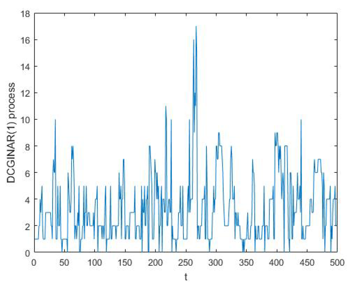
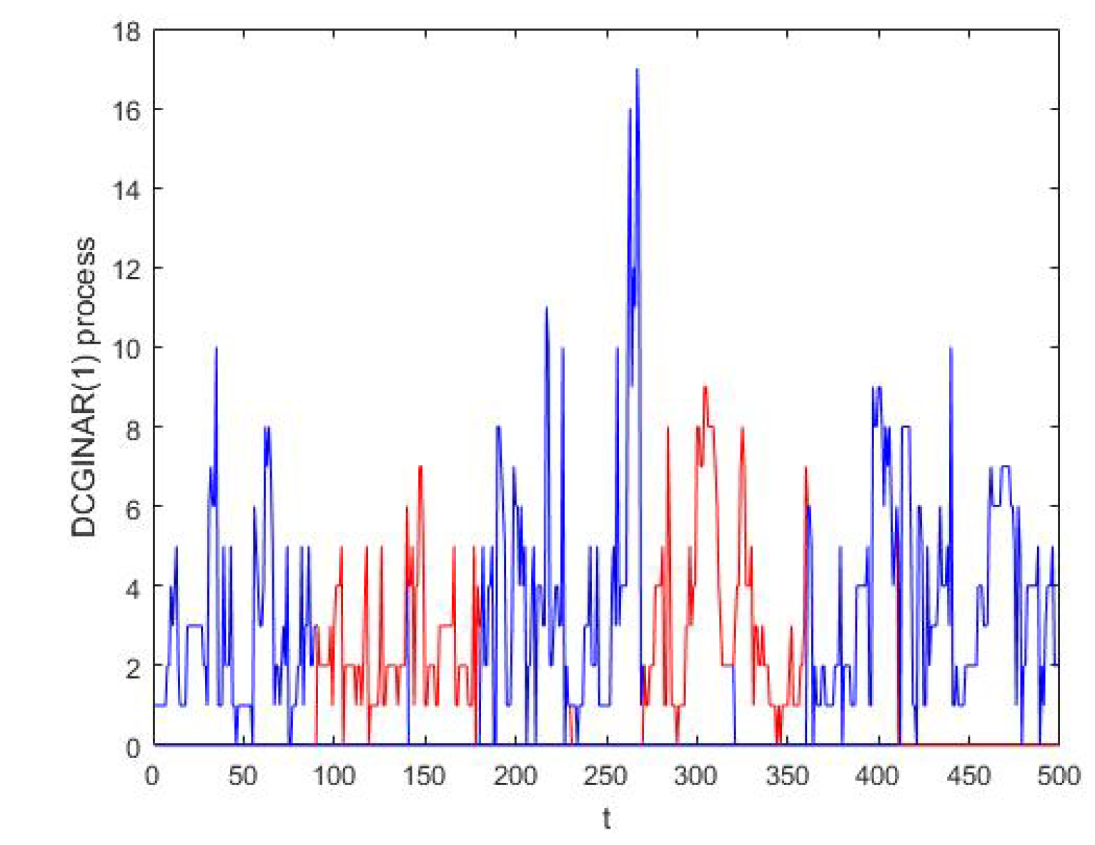
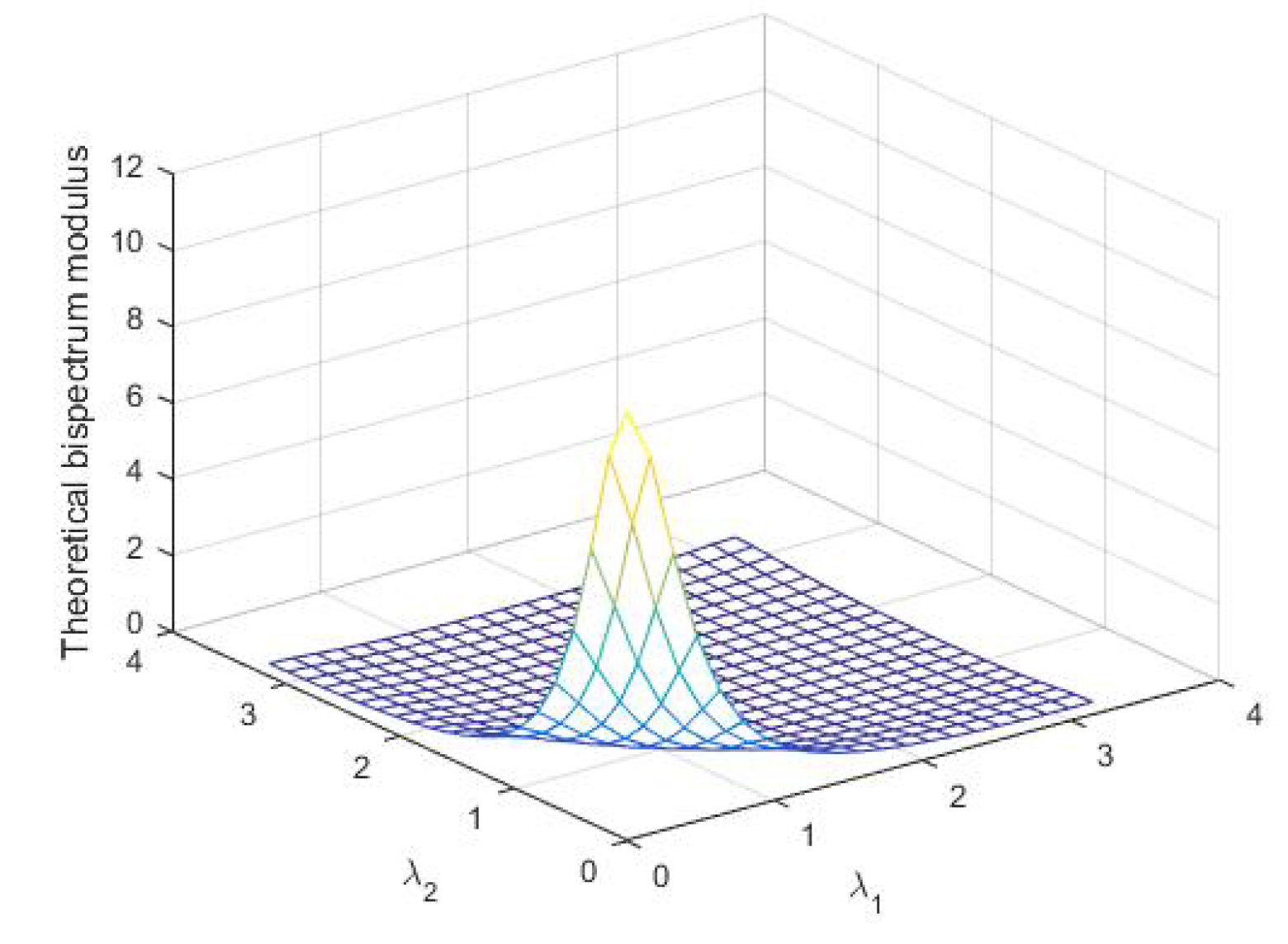
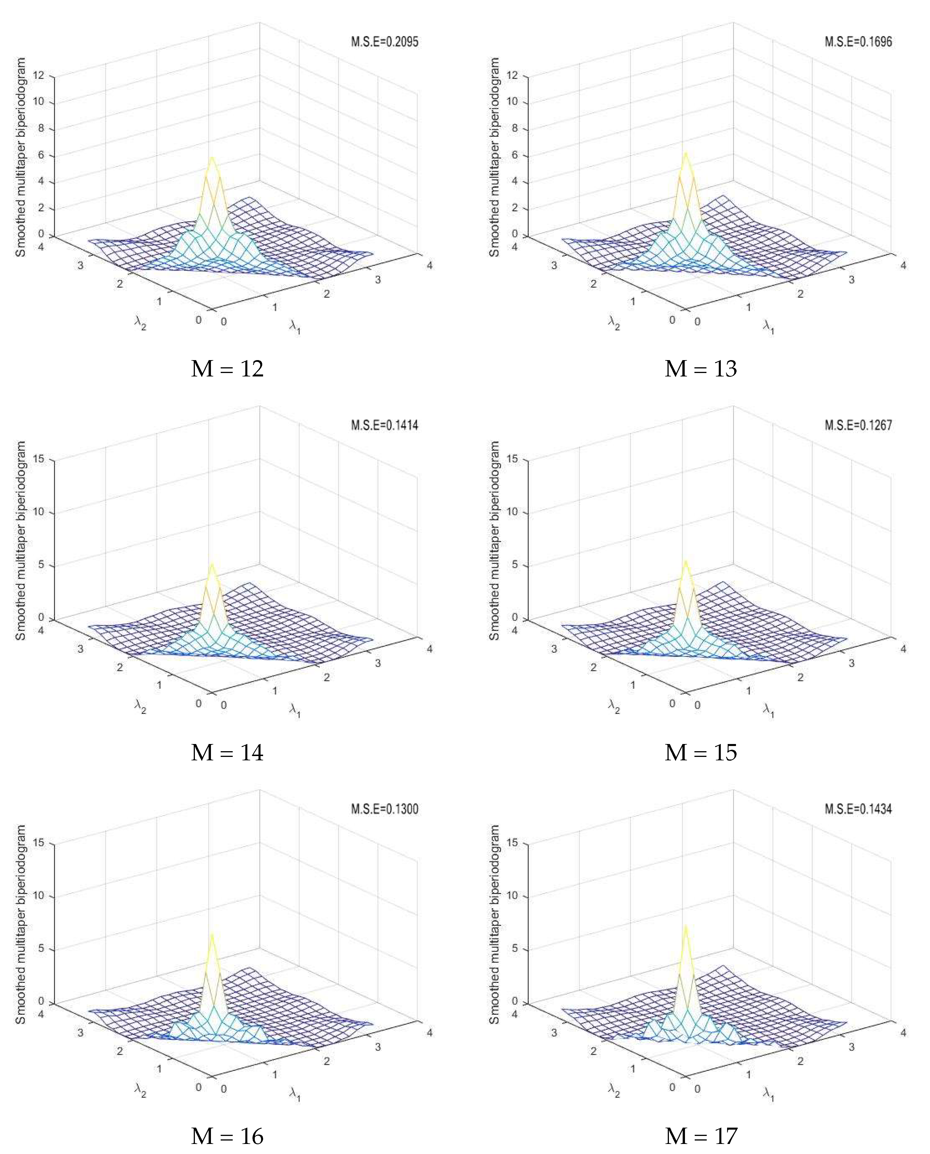
The estimate of the bispectral density function is calculated using the smoothed periodogram method in (13) and simulated series from the DCGINAR(1) model. Figure 1 represents the simulated series of $\{X_t,t=1,2,\dots ,500\}$ from the DCGINAR(1) model with $\mu =1.8,\alpha =0.6$ and $\theta =0.7$. From Figure 1, we note that the process is stationary, and values of simulated series are nonnegative integers, so the plot satisfies the definition of the DCGINAR(1) model. Figure 2 represents the same simulated series of $\{X_t,t=1,2,\dots ,500\}$ from the DCGINAR(1) model at $n=90,q=50$ and $L=5.$ The theoretical bispectrum $f_{XXX}({\lambda }_1,{\lambda }_2)$ is calculated by setting $\mu =1.8,\alpha =0.6$ and $\theta =0.7$ in (29). Figure 3 represents the theoretical bispectral modulus of the DCGINAR(1). Figure 4 represents the smoothed multitapered biperiodogram (which is the estimate of the bispectral density function of DCGINAR(1) model) with $\beta =0.09$ and different values of M using (6), (13) and (14).

Figure 1. The simulated series of the DCGINAR(1) model at $\alpha =0.6,\theta =0.7$.

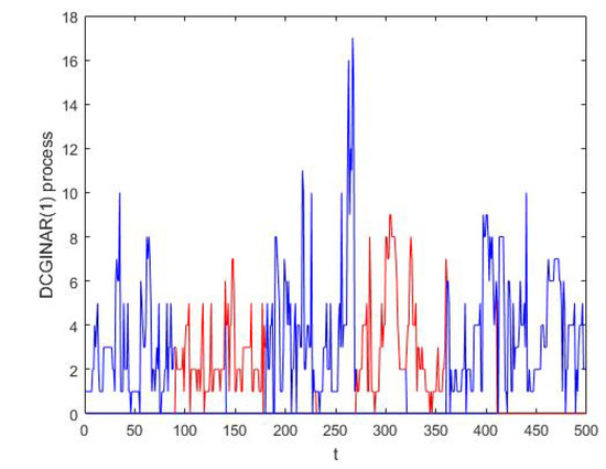
Figure 2. The overlapped segments for the same simulated series of the DCGINAR(1) model at $n=90,q=50$ and $L=5$.

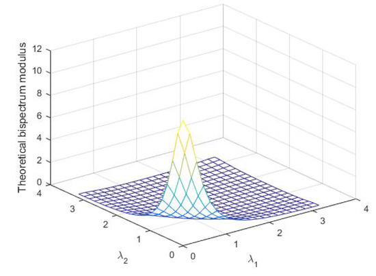
Figure 3. The theoretical bisectral modulus of the DCGINAR(1).

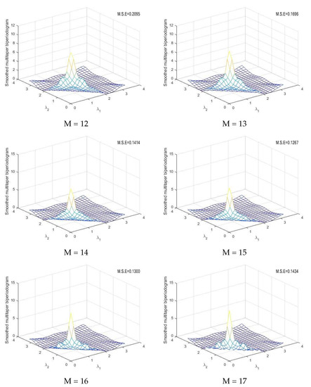
Figure 4. Smoothed multitaper biperiodogram at different values of M .

Some numerical values of theoretical bispectrum modulus as well as smoothed multitapered biperiodograms for the DCGINAR(1) are listed in Table 1, Table 2, Table 3, Table 4, Table 5, Table 6 and Table 7. It is found that the best value for the referred data is M = 15. The sample mean square error (M.S.E.) criterion are used to examine the accuracy of ${\widehat{f}}_{XXX}^{{\left(mt\right)}_{sp}}({\lambda }_1,{\lambda }_2)$ as an estimate of $f_{XXX}({\lambda }_1,{\lambda }_2)$ and compare the bispectral estimates of various simulations. This sample M.S.E. is defined as

$$M.S.E=\frac{1}{k}\sum _{i=1}^k\sum _{j=1}^k\left(\right|{\widehat{f}}_{XXX}^{{\left(mt\right)}_{sp}}({\lambda }_i,{\lambda }_j)|-|f_{XXX}({\lambda }_i,{\lambda }_j){\left|\right)}^2,$$

(32)

where $|{\widehat{f}}_{XXX}^{{\left(mt\right)}_{sp}}({\lambda }_i,{\lambda }_j)|$ is the modulus of the bispectral density estimate, and $|f_{XXX}({\lambda }_i,{\lambda }_j)|$ is the modulus of the theoretical bispectral density function. The summations are taken over all the frequencies (${\lambda }_i$,${\lambda }_j$), ${\lambda }_i$,${\lambda }_j$ = 0.00(0.05$\pi$)$\pi$, and k is the total number of these frequencies $({\lambda }_i,{\lambda }_j)$. Depending on the M.S.E value calculated from (32), which appears on each image, if we compare the estimated bispectrum modulus at different values of M in Figure 4 with the theoretical bispectrum modulus in Figure 3, we can conclude that $M=15$ is the best value for estimating the bispectrum modulus here. Using the smoothed multitapered biperiodogram at $M=15$ made the estimated bispectrum more similar to the theoretical bispectrum.

Table 1. Numerical values of theoretical bispectrum modulus of the DCGINAR(1) at $\mu =1.8,\alpha =0.6$ and $\theta =0.7$.

	${\mathit{\lambda }}_2$	0	0.05$\mathit{\pi }$	0.10$\mathit{\pi }$	0.15$\mathit{\pi }$	0.20$\mathit{\pi }$	0.25$\mathit{\pi }$	0.30$\mathit{\pi }$	0.35$\mathit{\pi }$	0.40$\mathit{\pi }$	0.45$\mathit{\pi }$	0.50$\mathit{\pi }$	0.55$\mathit{\pi }$	0.60$\mathit{\pi }$	0.65$\mathit{\pi }$	0.70$\mathit{\pi }$	0.75$\mathit{\pi }$	0.80$\mathit{\pi }$	0.85$\mathit{\pi }$	0.90$\mathit{\pi }$	0.95$\mathit{\pi }$	$\mathit{\pi }$
${\mathbf{\lambda }}_{\mathbf{1}}$
0		11.2352	9.9030	7.2167	4.8711	3.2912	2.3014	1.6801	1.2790	1.0108	0.8254	0.6933	0.5969	0.5252	0.4712	0.4302	0.3991	0.3759	0.3590	0.3476	0.3410	0.3388
0.05$\mathbf{\pi }$		9.9030	7.9364	5.5644	3.7554	2.5791	1.8410	1.3712	1.0627	0.8530	0.7060	0.6001	0.5220	0.4636	0.4194	0.3859	0.3607	0.3421	0.3289	0.3205	0.3164	0.3164
0.10$\mathbf{\pi }$		7.2167	5.5644	3.8987	2.6715	1.8703	1.3599	1.0296	0.8093	0.6577	0.5502	0.4721	0.4142	0.3708	0.3379	0.3130	0.2945	0.2811	0.2720	0.2667	0.2650	0.2667
0.15$\mathbf{\pi }$		4.8711	3.7554	2.6715	1.8651	1.3289	0.9812	0.7527	0.5984	0.4911	0.4145	0.3585	0.3168	0.2855	0.2619	0.2442	0.2312	0.2220	0.2161	0.2133	0.2133	0.2161
0.20$\mathbf{\pi }$		3.2912	2.5791	1.8703	1.3289	0.9612	0.7188	0.5574	0.4473	0.3701	0.3147	0.2741	0.2438	0.2211	0.2041	0.1914	0.1823	0.1761	0.1725	0.1714	0.1725	0.1761
0.25$\mathbf{\pi }$		2.3014	1.8410	1.3599	0.9812	0.7188	0.5432	0.4251	0.3438	0.2866	0.2453	0.2150	0.1924	0.1755	0.1629	0.1537	0.1473	0.1432	0.1412	0.1412	0.1432	0.1473
0.30$\mathbf{\pi }$		1.6801	1.3712	1.0296	0.7527	0.5574	0.4251	0.3352	0.2731	0.2291	0.1973	0.1739	0.1566	0.1437	0.1342	0.1274	0.1228	0.1201	0.1193	0.1201	0.1228	0.1274
0.35$\mathbf{\pi }$		1.2790	1.0627	0.8093	0.5984	0.4473	0.3438	0.2731	0.2239	0.1890	0.1637	0.1452	0.1314	0.1213	0.1140	0.1088	0.1056	0.1040	0.1040	0.1056	0.1088	0.1140
0.40$\mathbf{\pi }$		1.0108	0.8530	0.6577	0.4911	0.3701	0.2866	0.2291	0.1890	0.1604	0.1398	0.1247	0.1135	0.1054	0.0996	0.0958	0.0935	0.0928	0.0935	0.0958	0.0996	0.1054
0.45$\mathbf{\pi }$		0.8254	0.7060	0.5502	0.4145	0.3147	0.2453	0.1973	0.1637	0.1398	0.1225	0.1099	0.1007	0.0940	0.0894	0.0866	0.0852	0.0852	0.0866	0.0894	0.0940	0.1007
0.50$\mathbf{\pi }$		0.6933	0.6001	0.4721	0.3585	0.2741	0.2150	0.1739	0.1452	0.1247	0.1099	0.0991	0.0914	0.0859	0.0823	0.0802	0.0795	0.0802	0.0823	0.0859	0.0914	0.0991
0.55$\mathbf{\pi }$		0.5969	0.5220	0.4142	0.3168	0.2438	0.1924	0.1566	0.1314	0.1135	0.1007	0.0914	0.0848	0.0802	0.0774	0.0760	0.0760	0.0774	0.0802	0.0848	0.0914	0.1007
0.60$\mathbf{\pi }$		0.5252	0.4636	0.3708	0.2855	0.2211	0.1755	0.1437	0.1213	0.1054	0.0940	0.0859	0.0802	0.0765	0.0744	0.0737	0.0744	0.0765	0.0802	0.0859	0.0940	0.1054
0.65$\mathbf{\pi }$		0.4712	0.4194	0.3379	0.2619	0.2041	0.1629	0.1342	0.1140	0.0996	0.0894	0.0823	0.0774	0.0744	0.0729	0.0729	0.0744	0.0774	0.0823	0.0894	0.0996	0.1140
0.70$\mathbf{\pi }$		0.4302	0.3859	0.3130	0.2442	0.1914	0.1537	0.1274	0.1088	0.0958	0.0866	0.0802	0.0760	0.0737	0.0729	0.0737	0.0760	0.0802	0.0866	0.0958	0.1088	0.1274
0.75$\mathbf{\pi }$		0.3991	0.3607	0.2945	0.2312	0.1823	0.1473	0.1228	0.1056	0.0935	0.0852	0.0795	0.0760	0.0744	0.0744	0.0760	0.0795	0.0852	0.0935	0.1056	0.1228	0.1473
0.80$\mathbf{\pi }$		0.3759	0.3421	0.2811	0.2220	0.1761	0.1432	0.1201	0.1040	0.0928	0.0852	0.0802	0.0774	0.0765	0.0774	0.0802	0.0852	0.0928	0.1040	0.1201	0.1432	0.1761
0.85$\mathbf{\pi }$		0.3590	0.3289	0.2720	0.2161	0.1725	0.1412	0.1193	0.1040	0.0935	0.0866	0.0823	0.0802	0.0802	0.0823	0.0866	0.0935	0.1040	0.1193	0.1412	0.1725	0.2161
0.90$\mathbf{\pi }$		0.3476	0.3205	0.2667	0.2133	0.1714	0.1412	0.1201	0.1056	0.0958	0.0894	0.0859	0.0848	0.0859	0.0894	0.0958	0.1056	0.1201	0.1412	0.1714	0.2133	0.2667
0.95$\mathbf{\pi }$		0.3410	0.3164	0.2650	0.2133	0.1725	0.1432	0.1228	0.1088	0.0996	0.0940	0.0914	0.0914	0.0940	0.0996	0.1088	0.1228	0.1432	0.1725	0.2133	0.2650	0.3164
$\mathbf{\pi }$		0.3388	0.3164	0.2667	0.2161	0.1761	0.1473	0.1274	0.1140	0.1054	0.1007	0.0991	0.1007	0.1054	0.1140	0.1274	0.1473	0.1761	0.2161	0.2667	0.3164	0.3388

Table 2. Numerical values of smoothed multitapered biperiodogram of DCGINAR(1) model with $M=12$ and $\beta =0.09$.

	${\mathit{\lambda }}_2$	0	0.05$\mathit{\pi }$	0.10$\mathit{\pi }$	0.15$\mathit{\pi }$	0.20$\mathit{\pi }$	0.25$\mathit{\pi }$	0.30$\mathit{\pi }$	0.35$\mathit{\pi }$	0.40$\mathit{\pi }$	0.45$\mathit{\pi }$	0.50$\mathit{\pi }$	0.55$\mathit{\pi }$	0.60$\mathit{\pi }$	0.65$\mathit{\pi }$	0.70$\mathit{\pi }$	0.75$\mathit{\pi }$	0.80$\mathit{\pi }$	0.85$\mathit{\pi }$	0.90$\mathit{\pi }$	0.95$\mathit{\pi }$	$\mathit{\pi }$
${\mathbf{\lambda }}_{\mathbf{1}}$
0		11.5611	9.8639	6.805	5.275	5.0508	4.3963	3.2455	2.5186	2.1825	1.7485	1.2759	0.899	0.4956	0.1455	0.031	0.0523	0.1327	0.3934	0.7266	0.8635	0.8596
0.05$\mathbf{\pi }$		9.8639	7.5674	5.5329	4.7663	4.3513	3.4883	2.6402	2.1651	1.804	1.3793	0.989	0.6164	0.248	0.0617	0.0367	0.0764	0.2108	0.4938	0.7315	0.7956	0.7956
0.10$\mathbf{\pi }$		6.805	5.5329	4.4949	3.6911	3.1039	2.5518	2.041	1.6091	1.2796	0.9615	0.6098	0.2774	0.0947	0.0663	0.0486	0.1093	0.238	0.447	0.6061	0.6621	0.6061
0.15$\mathbf{\pi }$		5.275	4.7663	3.6911	2.7918	2.4084	2.0923	1.6085	1.2101	0.946	0.6288	0.291	0.1124	0.1078	0.0936	0.074	0.1313	0.2286	0.3926	0.5349	0.5349	0.3926
0.20$\mathbf{\pi }$		5.0508	4.3513	3.1039	2.4084	2.1953	1.8327	1.3443	0.9943	0.6876	0.3333	0.1309	0.1422	0.1689	0.158	0.0986	0.14	0.2229	0.3851	0.4803	0.3851	0.2229
0.25$\mathbf{\pi }$		4.3963	3.4883	2.5518	2.0923	1.8327	1.4598	1.0525	0.6889	0.3474	0.1427	0.1584	0.2125	0.2723	0.2004	0.1002	0.1297	0.2081	0.3296	0.3296	0.2081	0.1297
0.30$\mathbf{\pi }$		3.2455	2.6402	2.041	1.6085	1.3443	1.0525	0.6715	0.3207	0.1371	0.1593	0.2179	0.315	0.3177	0.1877	0.0858	0.1116	0.1642	0.2084	0.1642	0.1116	0.0858
0.35$\mathbf{\pi }$		2.5186	2.1651	1.6091	1.2101	0.9943	0.6889	0.3207	0.1299	0.1565	0.2244	0.3306	0.3767	0.3048	0.1649	0.0759	0.0905	0.1066	0.1066	0.0905	0.0759	0.1649
0.40$\mathbf{\pi }$		2.1825	1.804	1.2796	0.946	0.6876	0.3474	0.1371	0.1565	0.2331	0.3603	0.4181	0.3822	0.2832	0.1539	0.065	0.0621	0.0575	0.0621	0.065	0.1539	0.2832
0.45$\mathbf{\pi }$		1.7485	1.3793	0.9615	0.6288	0.3333	0.1427	0.1593	0.2244	0.3603	0.4384	0.4081	0.3417	0.2543	0.1264	0.0427	0.032	0.032	0.0427	0.1264	0.2543	0.3417
0.50$\mathbf{\pi }$		1.2759	0.989	0.6098	0.291	0.1309	0.1584	0.2179	0.3306	0.4181	0.4081	0.348	0.2927	0.1993	0.0795	0.0212	0.0172	0.0212	0.0795	0.1993	0.2927	0.348
0.55$\mathbf{\pi }$		0.899	0.6164	0.2774	0.1124	0.1422	0.2125	0.315	0.3767	0.3822	0.3417	0.2927	0.2252	0.123	0.0387	0.0112	0.0112	0.0387	0.123	0.2252	0.2927	0.3417
0.60$\mathbf{\pi }$		0.4956	0.248	0.0947	0.1078	0.1689	0.2723	0.3177	0.3048	0.2832	0.2543	0.1993	0.123	0.053	0.018	0.0063	0.018	0.053	0.123	0.1993	0.2543	0.2832
0.65$\mathbf{\pi }$		0.1455	0.0617	0.0663	0.0936	0.158	0.2004	0.1877	0.1649	0.1539	0.1264	0.0795	0.0387	0.018	0.0075	0.0075	0.018	0.0387	0.0795	0.1264	0.1539	0.1649
0.70$\mathbf{\pi }$		0.031	0.0367	0.0486	0.074	0.0986	0.1002	0.0858	0.0759	0.065	0.0427	0.0212	0.0112	0.0063	0.0075	0.0063	0.0112	0.0212	0.0427	0.065	0.0759	0.0858
0.75$\mathbf{\pi }$		0.0523	0.0764	0.1093	0.1313	0.14	0.1297	0.1116	0.0905	0.0621	0.032	0.0172	0.0112	0.018	0.018	0.0112	0.0172	0.032	0.0621	0.0905	0.1116	0.1297
0.80$\mathbf{\pi }$		0.1327	0.2108	0.238	0.2286	0.2229	0.2081	0.1642	0.1066	0.0575	0.032	0.0212	0.0387	0.053	0.0387	0.0212	0.032	0.0575	0.1066	0.1642	0.2081	0.2229
0.85$\mathbf{\pi }$		0.3934	0.4938	0.447	0.3926	0.3851	0.3296	0.2084	0.1066	0.0621	0.0427	0.0795	0.123	0.123	0.0795	0.0427	0.0621	0.1066	0.2084	0.3296	0.3851	0.3926
0.90$\mathbf{\pi }$		0.7266	0.7315	0.6061	0.5349	0.4803	0.3296	0.1642	0.0905	0.065	0.1264	0.1993	0.2252	0.1993	0.1264	0.065	0.0905	0.1642	0.3296	0.4803	0.5349	0.6061
0.95$\mathbf{\pi }$		0.8635	0.7956	0.6621	0.5349	0.3851	0.2081	0.1116	0.0759	0.1539	0.2543	0.2927	0.2927	0.2543	0.1539	0.0759	0.1116	0.2081	0.3851	0.5349	0.6621	0.7956
$\mathbf{\pi }$		0.8596	0.7956	0.6061	0.3926	0.2229	0.1297	0.0858	0.1649	0.2832	0.3417	0.348	0.3417	0.2832	0.1649	0.0858	0.1297	0.2229	0.3926	0.6061	0.7956	0.8596

Table 3. Numerical values of smoothed multitapered biperiodogram of DCGINAR(1) model with $M=13$ and $\beta =0.09$.

	${\mathit{\lambda }}_2$	0	0.05$\mathit{\pi }$	0.10$\mathit{\pi }$	0.15$\mathit{\pi }$	0.20$\mathit{\pi }$	0.25$\mathit{\pi }$	0.30$\mathit{\pi }$	0.35$\mathit{\pi }$	0.40$\mathit{\pi }$	0.45$\mathit{\pi }$	0.50$\mathit{\pi }$	0.55$\mathit{\pi }$	0.60$\mathit{\pi }$	0.65$\mathit{\pi }$	0.70$\mathit{\pi }$	0.75$\mathit{\pi }$	0.80$\mathit{\pi }$	0.85$\mathit{\pi }$	0.90$\mathit{\pi }$	0.95$\mathit{\pi }$	$\mathit{\pi }$
${\mathbf{\lambda }}_{\mathbf{1}}$
0		11.8543	9.8299	6.4759	5.1308	4.8888	4.0414	3.1227	2.6088	2.0355	1.5383	1.3358	0.973	0.4167	0.1198	0.0449	0.0224	0.1698	0.4111	0.6113	0.8491	0.992
0.05$\mathbf{\pi }$		9.8299	7.265	5.2475	4.5589	4.0463	3.2341	2.5984	2.0978	1.6109	1.3051	1.038	0.5797	0.2031	0.0663	0.0285	0.056	0.2405	0.4563	0.6559	0.8357	0.8357
0.10$\mathbf{\pi }$		6.4759	5.2475	4.1552	3.3621	2.8863	2.3991	1.8622	1.4797	1.2184	0.904	0.5513	0.252	0.1004	0.0379	0.0641	0.0708	0.2379	0.4365	0.5755	0.6275	0.5755
0.15$\mathbf{\pi }$		5.1308	4.5589	3.3621	2.6317	2.3501	1.8867	1.4409	1.2279	0.926	0.5266	0.2631	0.1371	0.0633	0.0934	0.0888	0.0769	0.2497	0.4201	0.4738	0.4738	0.4201
0.20$\mathbf{\pi }$		4.8888	4.0463	2.8863	2.3501	2.0266	1.6006	1.3111	1.0234	0.5913	0.275	0.1567	0.0944	0.1708	0.1419	0.1057	0.0882	0.2636	0.3792	0.392	0.3792	0.2636
0.25$\mathbf{\pi }$		4.0414	3.2341	2.3991	1.8867	1.6006	1.3558	1.0176	0.6087	0.2874	0.1524	0.1007	0.2373	0.2416	0.1576	0.1133	0.0867	0.2216	0.2922	0.2922	0.2216	0.0867
0.30$\mathbf{\pi }$		3.1227	2.5984	1.8622	1.4409	1.3111	1.0176	0.5854	0.2866	0.1543	0.095	0.2442	0.3242	0.259	0.1633	0.1076	0.0707	0.1652	0.2107	0.1652	0.0707	0.1076
0.35$\mathbf{\pi }$		2.6088	2.0978	1.4797	1.2279	1.0234	0.6087	0.2866	0.1601	0.0997	0.2396	0.347	0.3613	0.279	0.1612	0.091	0.0547	0.124	0.124	0.0547	0.091	0.1612
0.40$\mathbf{\pi }$		2.0355	1.6109	1.2184	0.926	0.5913	0.2874	0.1543	0.0997	0.2437	0.3294	0.3742	0.3766	0.2664	0.1319	0.0682	0.0395	0.0704	0.0395	0.0682	0.1319	0.2664
0.45$\mathbf{\pi }$		1.5383	1.3051	0.904	0.5266	0.275	0.1524	0.095	0.2396	0.3294	0.3493	0.3836	0.3539	0.2143	0.0974	0.0487	0.0221	0.0221	0.0487	0.0974	0.2143	0.3539
0.50$\mathbf{\pi }$		1.3358	1.038	0.5513	0.2631	0.1567	0.1007	0.2442	0.347	0.3742	0.3836	0.3862	0.3049	0.1694	0.0744	0.0292	0.0075	0.0292	0.0744	0.1694	0.3049	0.3862
0.55$\mathbf{\pi }$		0.973	0.5797	0.252	0.1371	0.0944	0.2373	0.3242	0.3613	0.3766	0.3539	0.3049	0.2209	0.1185	0.0408	0.009	0.009	0.0408	0.1185	0.2209	0.3049	0.3539
0.60$\mathbf{\pi }$		0.4167	0.2031	0.1004	0.0633	0.1708	0.2416	0.259	0.279	0.2664	0.2143	0.1694	0.1185	0.0498	0.0097	0.0084	0.0097	0.0498	0.1185	0.1694	0.2143	0.2664
0.65$\mathbf{\pi }$		0.1198	0.0663	0.0379	0.0934	0.1419	0.1576	0.1633	0.1612	0.1319	0.0974	0.0744	0.0408	0.0097	0.0072	0.0072	0.0097	0.0408	0.0744	0.0974	0.1319	0.1612
0.70$\mathbf{\pi }$		0.0449	0.0285	0.0641	0.0888	0.1057	0.1133	0.1076	0.091	0.0682	0.0487	0.0292	0.009	0.0084	0.0072	0.0084	0.009	0.0292	0.0487	0.0682	0.091	0.1076
0.75$\mathbf{\pi }$		0.0224	0.056	0.0708	0.0769	0.0882	0.0867	0.0707	0.0547	0.0395	0.0221	0.0075	0.009	0.0097	0.0097	0.009	0.0075	0.0221	0.0395	0.0547	0.0707	0.0867
0.80$\mathbf{\pi }$		0.1698	0.2405	0.2379	0.2497	0.2636	0.2216	0.1652	0.124	0.0704	0.0221	0.0292	0.0408	0.0498	0.0408	0.0292	0.0221	0.0704	0.124	0.1652	0.2216	0.2636
0.85$\mathbf{\pi }$		0.4111	0.4563	0.4365	0.4201	0.3792	0.2922	0.2107	0.124	0.0395	0.0487	0.0744	0.1185	0.1185	0.0744	0.0487	0.0395	0.124	0.2107	0.2922	0.3792	0.4201
0.90$\mathbf{\pi }$		0.6113	0.6559	0.5755	0.4738	0.392	0.2922	0.1652	0.0547	0.0682	0.0974	0.1694	0.2209	0.1694	0.0974	0.0682	0.0547	0.1652	0.2922	0.392	0.4738	0.5755
0.95$\mathbf{\pi }$		0.8491	0.8357	0.6275	0.4738	0.3792	0.2216	0.0707	0.091	0.1319	0.2143	0.3049	0.3049	0.2143	0.1319	0.091	0.0707	0.2216	0.3792	0.4738	0.6275	0.8357
$\mathbf{\pi }$		0.992	0.8357	0.5755	0.4201	0.2636	0.0867	0.1076	0.1612	0.2664	0.3539	0.3862	0.3539	0.2664	0.1612	0.1076	0.0867	0.2636	0.4201	0.5755	0.8357	0.992

Table 4. Numerical values of smoothed multitapered biperiodogram of DCGINAR(1) model with $M=14$ and $\beta =0.09$.

	${\mathit{\lambda }}_2$	0	0.05$\mathit{\pi }$	0.10$\mathit{\pi }$	0.15$\mathit{\pi }$	0.20$\mathit{\pi }$	0.25$\mathit{\pi }$	0.30$\mathit{\pi }$	0.35$\mathit{\pi }$	0.40$\mathit{\pi }$	0.45$\mathit{\pi }$	0.50$\mathit{\pi }$	0.55$\mathit{\pi }$	0.60$\mathit{\pi }$	0.65$\mathit{\pi }$	0.70$\mathit{\pi }$	0.75$\mathit{\pi }$	0.80$\mathit{\pi }$	0.85$\mathit{\pi }$	0.90$\mathit{\pi }$	0.95$\mathit{\pi }$	$\mathit{\pi }$
${\mathbf{\lambda }}_{\mathbf{1}}$
0		12.1855	9.7818	6.1558	5.0108	4.6472	3.7593	3.1864	2.5834	1.7753	1.535	1.43	0.8699	0.3765	0.1561	0.0212	0.0401	0.1436	0.3453	0.6957	0.8756	0.8651
0.05$\mathbf{\pi }$		9.7818	6.9518	4.9739	4.3212	3.7435	3.1001	2.5697	1.9182	1.4788	1.3272	0.9991	0.5125	0.2168	0.0514	0.0261	0.0678	0.1993	0.439	0.6992	0.7797	0.7797
0.10$\mathbf{\pi }$		6.1558	4.9739	3.797	3.0813	2.7342	2.214	1.6891	1.4148	1.1323	0.821	0.5214	0.2614	0.0633	0.056	0.0392	0.0833	0.2245	0.3907	0.5512	0.6223	0.5512
0.15$\mathbf{\pi }$		5.0108	4.3212	3.0813	2.5621	2.2229	1.6558	1.4176	1.2327	0.7966	0.4873	0.303	0.087	0.0785	0.0955	0.0548	0.107	0.2274	0.3502	0.5004	0.5004	0.3502
0.20$\mathbf{\pi }$		4.6472	3.7435	2.7342	2.2229	1.7738	1.4826	1.3182	0.9256	0.5041	0.302	0.1075	0.1151	0.1432	0.1431	0.075	0.1156	0.2172	0.3393	0.4296	0.3393	0.2172
0.25$\mathbf{\pi }$		3.7593	3.1001	2.214	1.6558	1.4826	1.2874	0.9246	0.5472	0.2917	0.1001	0.1327	0.1961	0.2002	0.1827	0.0756	0.1031	0.1965	0.2721	0.2721	0.1965	0.1031
0.30$\mathbf{\pi }$		3.1864	2.5697	1.6891	1.4176	1.3182	0.9246	0.5601	0.3246	0.0991	0.1265	0.2312	0.2802	0.2613	0.1884	0.0692	0.0956	0.1615	0.1766	0.1615	0.0956	0.0692
0.35$\mathbf{\pi }$		2.5834	1.9182	1.4148	1.2327	0.9256	0.5472	0.3246	0.1078	0.1227	0.2157	0.3233	0.3581	0.2639	0.1688	0.0627	0.0768	0.1023	0.1023	0.0768	0.0627	0.1688
0.40$\mathbf{\pi }$		1.7753	1.4788	1.1323	0.7966	0.5041	0.2917	0.0991	0.1227	0.1926	0.2778	0.3807	0.3331	0.2178	0.141	0.0463	0.0448	0.0545	0.0448	0.0463	0.141	0.2178
0.45$\mathbf{\pi }$		1.535	1.3272	0.821	0.4873	0.302	0.1001	0.1265	0.2157	0.2778	0.3667	0.397	0.3079	0.2037	0.1168	0.0303	0.0269	0.0269	0.0303	0.1168	0.2037	0.3079
0.50$\mathbf{\pi }$		1.43	0.9991	0.5214	0.303	0.1075	0.1327	0.2312	0.3233	0.3807	0.397	0.3808	0.2989	0.1752	0.0794	0.0189	0.0138	0.0189	0.0794	0.1752	0.2989	0.3808
0.55$\mathbf{\pi }$		0.8699	0.5125	0.2614	0.087	0.1151	0.1961	0.2802	0.3581	0.3331	0.3079	0.2989	0.2078	0.0963	0.04	0.0078	0.0078	0.04	0.0963	0.2078	0.2989	0.3079
0.60$\mathbf{\pi }$		0.3765	0.2168	0.0633	0.0785	0.1432	0.2002	0.2613	0.2639	0.2178	0.2037	0.1752	0.0963	0.0409	0.0138	0.0037	0.0138	0.0409	0.0963	0.1752	0.2037	0.2178
0.65$\mathbf{\pi }$		0.1561	0.0514	0.056	0.0955	0.1431	0.1827	0.1884	0.1688	0.141	0.1168	0.0794	0.04	0.0138	0.0065	0.0065	0.0138	0.04	0.0794	0.1168	0.141	0.1688
0.70$\mathbf{\pi }$		0.0212	0.0261	0.0392	0.0548	0.075	0.0756	0.0692	0.0627	0.0463	0.0303	0.0189	0.0078	0.0037	0.0065	0.0037	0.0078	0.0189	0.0303	0.0463	0.0627	0.0692
0.75$\mathbf{\pi }$		0.0401	0.0678	0.0833	0.107	0.1156	0.1031	0.0956	0.0768	0.0448	0.0269	0.0138	0.0078	0.0138	0.0138	0.0078	0.0138	0.0269	0.0448	0.0768	0.0956	0.1031
0.80$\mathbf{\pi }$		0.1436	0.1993	0.2245	0.2274	0.2172	0.1965	0.1615	0.1023	0.0545	0.0269	0.0189	0.04	0.0409	0.04	0.0189	0.0269	0.0545	0.1023	0.1615	0.1965	0.2172
0.85$\mathbf{\pi }$		0.3453	0.439	0.3907	0.3502	0.3393	0.2721	0.1766	0.1023	0.0448	0.0303	0.0794	0.0963	0.0963	0.0794	0.0303	0.0448	0.1023	0.1766	0.2721	0.3393	0.3502
0.90$\mathbf{\pi }$		0.6957	0.6992	0.5512	0.5004	0.4296	0.2721	0.1615	0.0768	0.0463	0.1168	0.1752	0.2078	0.1752	0.1168	0.0463	0.0768	0.1615	0.2721	0.4296	0.5004	0.5512
0.95$\mathbf{\pi }$		0.8756	0.7797	0.6223	0.5004	0.3393	0.1965	0.0956	0.0627	0.141	0.2037	0.2989	0.2989	0.2037	0.141	0.0627	0.0956	0.1965	0.3393	0.5004	0.6223	0.7797
$\mathbf{\pi }$		0.8651	0.7797	0.5512	0.3502	0.2172	0.1031	0.0692	0.1688	0.2178	0.3079	0.3808	0.3079	0.2178	0.1688	0.0692	0.1031	0.2172	0.3502	0.5512	0.7797	0.8651

Table 5. Numerical values of smoothed multitapered biperiodogram of DCGINAR(1) model with $M=15$ and $\beta =0.09$.

	${\mathit{\lambda }}_2$	0	0.05$\mathit{\pi }$	0.10$\mathit{\pi }$	0.15$\mathit{\pi }$	0.20$\mathit{\pi }$	0.25$\mathit{\pi }$	0.30$\mathit{\pi }$	0.35$\mathit{\pi }$	0.40$\mathit{\pi }$	0.45$\mathit{\pi }$	0.50$\mathit{\pi }$	0.55$\mathit{\pi }$	0.60$\mathit{\pi }$	0.65$\mathit{\pi }$	0.70$\mathit{\pi }$	0.75$\mathit{\pi }$	0.80$\mathit{\pi }$	0.85$\mathit{\pi }$	0.90$\mathit{\pi }$	0.95$\mathit{\pi }$	$\mathit{\pi }$
${\mathbf{\lambda }}_{\mathbf{1}}$
0		12.5334	9.7103	5.8637	4.8954	4.3392	3.6252	3.307	2.3805	1.6303	1.6359	1.3316	0.8026	0.443	0.1251	0.0185	0.0278	0.1274	0.4105	0.6202	0.8232	0.9779
0.05$\mathbf{\pi }$		9.7103	6.6408	4.7131	4.0541	3.4897	3.0468	2.4689	1.7336	1.4372	1.2988	0.9097	0.5245	0.207	0.0422	0.0197	0.0522	0.2012	0.444	0.6288	0.7897	0.7897
0.10$\mathbf{\pi }$		5.8637	4.7131	3.4449	2.8787	2.5907	2.0082	1.5874	1.3495	1.0073	0.7834	0.5252	0.2164	0.0619	0.0401	0.033	0.073	0.1921	0.3975	0.5326	0.5629	0.5326
0.15$\mathbf{\pi }$		4.8954	4.0541	2.8787	2.5156	2.0091	1.5184	1.4537	1.1125	0.7144	0.5323	0.2551	0.076	0.0689	0.0789	0.0542	0.0819	0.2023	0.396	0.4463	0.4463	0.396
0.20$\mathbf{\pi }$		4.3392	3.4897	2.5907	2.0091	1.564	1.4323	1.2347	0.8125	0.4997	0.2662	0.0919	0.0875	0.1397	0.1334	0.0628	0.0885	0.2076	0.3419	0.3644	0.3419	0.2076
0.25$\mathbf{\pi }$		3.6252	3.0468	2.0082	1.5184	1.4323	1.1815	0.8759	0.5519	0.2427	0.0933	0.1031	0.1719	0.229	0.1497	0.0661	0.0883	0.1742	0.2711	0.2711	0.1742	0.0883
0.30$\mathbf{\pi }$		3.307	2.4689	1.5874	1.4537	1.2347	0.8759	0.6219	0.2803	0.0891	0.1091	0.2115	0.2944	0.2687	0.1648	0.0688	0.0775	0.1443	0.2109	0.1443	0.0775	0.0688
0.35$\mathbf{\pi }$		2.3805	1.7336	1.3495	1.1125	0.8125	0.5519	0.2803	0.0912	0.0924	0.1989	0.3222	0.3072	0.2631	0.1524	0.0536	0.0569	0.0996	0.0996	0.0569	0.0536	0.1524
0.40$\mathbf{\pi }$		1.6303	1.4372	1.0073	0.7144	0.4997	0.2427	0.0891	0.0924	0.1643	0.2954	0.3277	0.2931	0.2372	0.1157	0.0385	0.0384	0.0459	0.0384	0.0385	0.1157	0.2372
0.45$\mathbf{\pi }$		1.6359	1.2988	0.7834	0.5323	0.2662	0.0933	0.1091	0.1989	0.2954	0.3637	0.3782	0.3199	0.218	0.1006	0.0314	0.0214	0.0214	0.0314	0.1006	0.218	0.3199
0.50$\mathbf{\pi }$		1.3316	0.9097	0.5252	0.2551	0.0919	0.1031	0.2115	0.3222	0.3277	0.3782	0.3719	0.2649	0.1708	0.0738	0.0158	0.0089	0.0158	0.0738	0.1708	0.2649	0.3719
0.55$\mathbf{\pi }$		0.8026	0.5245	0.2164	0.076	0.0875	0.1719	0.2944	0.3072	0.2931	0.3199	0.2649	0.1786	0.1078	0.0319	0.0057	0.0057	0.0319	0.1078	0.1786	0.2649	0.3199
0.60$\mathbf{\pi }$		0.443	0.207	0.0619	0.0689	0.1397	0.229	0.2687	0.2631	0.2372	0.218	0.1708	0.1078	0.0446	0.0111	0.0034	0.0111	0.0446	0.1078	0.1708	0.218	0.2372
0.65$\mathbf{\pi }$		0.1251	0.0422	0.0401	0.0789	0.1334	0.1497	0.1648	0.1524	0.1157	0.1006	0.0738	0.0319	0.0111	0.0048	0.0048	0.0111	0.0319	0.0738	0.1006	0.1157	0.1524
0.70$\mathbf{\pi }$		0.0185	0.0197	0.033	0.0542	0.0628	0.0661	0.0688	0.0536	0.0385	0.0314	0.0158	0.0057	0.0034	0.0048	0.0034	0.0057	0.0158	0.0314	0.0385	0.0536	0.0688
0.75$\mathbf{\pi }$		0.0278	0.0522	0.073	0.0819	0.0885	0.0883	0.0775	0.0569	0.0384	0.0214	0.0089	0.0057	0.0111	0.0111	0.0057	0.0089	0.0214	0.0384	0.0569	0.0775	0.0883
0.80$\mathbf{\pi }$		0.1274	0.2012	0.1921	0.2023	0.2076	0.1742	0.1443	0.0996	0.0459	0.0214	0.0158	0.0319	0.0446	0.0319	0.0158	0.0214	0.0459	0.0996	0.1443	0.1742	0.2076
0.85$\mathbf{\pi }$		0.4105	0.444	0.3975	0.396	0.3419	0.2711	0.2109	0.0996	0.0384	0.0314	0.0738	0.1078	0.1078	0.0738	0.0314	0.0384	0.0996	0.2109	0.2711	0.3419	0.396
0.90$\mathbf{\pi }$		0.6202	0.6288	0.5326	0.4463	0.3644	0.2711	0.1443	0.0569	0.0385	0.1006	0.1708	0.1786	0.1708	0.1006	0.0385	0.0569	0.1443	0.2711	0.3644	0.4463	0.5326
0.99$\mathbf{\pi }$		0.8232	0.7897	0.5629	0.4463	0.3419	0.1742	0.0775	0.0536	0.1157	0.218	0.2649	0.2649	0.218	0.1157	0.0536	0.0775	0.1742	0.3419	0.4463	0.5629	0.7897
$\mathbf{\pi }$		0.9779	0.7897	0.5326	0.396	0.2076	0.0883	0.0688	0.1524	0.2372	0.3199	0.3719	0.3199	0.2372	0.1524	0.0688	0.0883	0.2076	0.396	0.5326	0.7897	0.9779

Table 6. Numerical values of smoothed multitapered biperiodogram of DCGINAR(1) model with $M=16$ and $\beta =0.09$.

	${\mathit{\lambda }}_2$	0	0.05$\mathit{\pi }$	0.10$\mathit{\pi }$	0.15$\mathit{\pi }$	0.20$\mathit{\pi }$	0.25$\mathit{\pi }$	0.30$\mathit{\pi }$	0.35$\mathit{\pi }$	0.40$\mathit{\pi }$	0.45$\mathit{\pi }$	0.50$\mathit{\pi }$	0.55$\mathit{\pi }$	0.60$\mathit{\pi }$	0.65$\mathit{\pi }$	0.70$\mathit{\pi }$	0.75$\mathit{\pi }$	0.80$\mathit{\pi }$	0.85$\mathit{\pi }$	0.90$\mathit{\pi }$	0.95$\mathit{\pi }$	$\mathit{\pi }$
${\mathbf{\lambda }}_{\mathbf{1}}$
0		13.4644	9.6273	5.5741	5.0625	3.9013	3.7343	3.5292	2.003	1.7797	1.6493	1.1196	1.0007	0.4267	0.0763	0.0502	0.0193	0.1917	0.278	0.7085	0.947	0.7685
0.05$\mathbf{\pi }$		9.6273	6.1914	4.4866	3.7537	3.2252	3.0682	2.2472	1.5952	1.4472	1.1478	0.8941	0.5519	0.1516	0.0514	0.0259	0.0507	0.1942	0.3745	0.692	0.7207	0.7207
0.10$\mathbf{\pi }$		5.5741	4.4866	2.9923	2.7953	2.3867	1.7578	1.6121	1.168	0.9068	0.8263	0.4439	0.1775	0.0935	0.0246	0.0627	0.0463	0.2367	0.3297	0.4741	0.6092	0.4741
0.15$\mathbf{\pi }$		5.0625	3.7537	2.7953	2.5937	1.7123	1.5801	1.4795	0.9168	0.8186	0.5145	0.1783	0.137	0.0551	0.0732	0.0715	0.0713	0.2614	0.2826	0.5023	0.5023	0.2826
0.20$\mathbf{\pi }$		3.9013	3.2252	2.3867	1.7123	1.4155	1.3354	1.0688	0.7609	0.4689	0.1893	0.1262	0.0743	0.1537	0.078	0.1006	0.0722	0.2055	0.2752	0.3813	0.2752	0.2055
0.25$\mathbf{\pi }$		3.7343	3.0682	1.7578	1.5801	1.3354	1.0764	0.9894	0.4865	0.1936	0.1505	0.0769	0.2295	0.1811	0.1219	0.114	0.0635	0.2239	0.2335	0.2335	0.2239	0.0635
0.30$\mathbf{\pi }$		3.5292	2.2472	1.6121	1.4795	1.0688	0.9894	0.6283	0.1991	0.1524	0.0905	0.2362	0.269	0.2814	0.1366	0.0995	0.0689	0.1886	0.1419	0.1886	0.0689	0.0995
0.35$\mathbf{\pi }$		2.003	1.5952	1.168	0.9168	0.7609	0.4865	0.1991	0.1211	0.071	0.2164	0.2152	0.3246	0.2451	0.0931	0.0834	0.0447	0.0884	0.0884	0.0447	0.0834	0.0931
0.40$\mathbf{\pi }$		1.7797	1.4472	0.9068	0.8186	0.4689	0.1936	0.1524	0.071	0.2116	0.2455	0.3235	0.3532	0.2079	0.0972	0.0682	0.0264	0.0697	0.0264	0.0682	0.0972	0.2079
0.45$\mathbf{\pi }$		1.6493	1.1478	0.8263	0.5145	0.1893	0.1505	0.0905	0.2164	0.2455	0.3778	0.36	0.3065	0.2221	0.081	0.0407	0.0213	0.0213	0.0407	0.081	0.2221	0.3065
0.50$\mathbf{\pi }$		1.1196	0.8941	0.4439	0.1783	0.1262	0.0769	0.2362	0.2152	0.3235	0.36	0.2678	0.2804	0.1584	0.042	0.028	0.0054	0.028	0.042	0.1584	0.2804	0.2678
0.55$\mathbf{\pi }$		1.0007	0.5519	0.1775	0.137	0.0743	0.2295	0.269	0.3246	0.3532	0.3065	0.2804	0.229	0.0937	0.0327	0.0084	0.0084	0.0327	0.0937	0.229	0.2804	0.3065
0.60$\mathbf{\pi }$		0.4267	0.1516	0.0935	0.0551	0.1537	0.1811	0.2814	0.2451	0.2079	0.2221	0.1584	0.0937	0.0507	0.0067	0.009	0.0067	0.0507	0.0937	0.1584	0.2221	0.2079
0.65$\mathbf{\pi }$		0.0763	0.0514	0.0246	0.0732	0.078	0.1219	0.1366	0.0931	0.0972	0.081	0.042	0.0327	0.0067	0.0045	0.0045	0.0067	0.0327	0.042	0.081	0.0972	0.0931
0.70$\mathbf{\pi }$		0.0502	0.0259	0.0627	0.0715	0.1006	0.114	0.0995	0.0834	0.0682	0.0407	0.028	0.0084	0.009	0.0045	0.009	0.0084	0.028	0.0407	0.0682	0.0834	0.0995
0.75$\mathbf{\pi }$		0.0193	0.0507	0.0463	0.0713	0.0722	0.0635	0.0689	0.0447	0.0264	0.0213	0.0054	0.0084	0.0067	0.0067	0.0084	0.0054	0.0213	0.0264	0.0447	0.0689	0.0635
0.80$\mathbf{\pi }$		0.1917	0.1942	0.2367	0.2614	0.2055	0.2239	0.1886	0.0884	0.0697	0.0213	0.028	0.0327	0.0507	0.0327	0.028	0.0213	0.0697	0.0884	0.1886	0.2239	0.2055
0.85$\mathbf{\pi }$		0.278	0.3745	0.3297	0.2826	0.2752	0.2335	0.1419	0.0884	0.0264	0.0407	0.042	0.0937	0.0937	0.042	0.0407	0.0264	0.0884	0.1419	0.2335	0.2752	0.2826
0.90$\mathbf{\pi }$		0.7085	0.692	0.4741	0.5023	0.3813	0.2335	0.1886	0.0447	0.0682	0.081	0.1584	0.229	0.1584	0.081	0.0682	0.0447	0.1886	0.2335	0.3813	0.5023	0.4741
0.95$\mathbf{\pi }$		0.947	0.7207	0.6092	0.5023	0.2752	0.2239	0.0689	0.0834	0.0972	0.2221	0.2804	0.2804	0.2221	0.0972	0.0834	0.0689	0.2239	0.2752	0.5023	0.6092	0.7207
$\mathbf{\pi }$		0.7685	0.7207	0.4741	0.2826	0.2055	0.0635	0.0995	0.0931	0.2079	0.3065	0.2678	0.3065	0.2079	0.0931	0.0995	0.0635	0.2055	0.2826	0.4741	0.7207	0.7685

Table 7. Numerical values of smoothed multitapered biperiodogram of DCGINAR(1) model with $M=17$ and $\beta =0.09$.

	${\mathit{\lambda }}_2$	0	0.05$\mathit{\pi }$	0.10$\mathit{\pi }$	0.15$\mathit{\pi }$	0.20$\mathit{\pi }$	0.25$\mathit{\pi }$	0.30$\mathit{\pi }$	0.35$\mathit{\pi }$	0.40$\mathit{\pi }$	0.45$\mathit{\pi }$	0.50$\mathit{\pi }$	0.55$\mathit{\pi }$	0.60$\mathit{\pi }$	0.65$\mathit{\pi }$	0.70$\mathit{\pi }$	0.75$\mathit{\pi }$	0.80$\mathit{\pi }$	0.85$\mathit{\pi }$	0.90$\mathit{\pi }$	0.95$\mathit{\pi }$	$\mathit{\pi }$
${\mathbf{\lambda }}_{\mathbf{1}}$
0		14.2824	9.4763	5.4075	5.0651	3.498	4.0708	3.3823	1.836	1.9688	1.3601	1.2737	1.0541	0.2942	0.1474	0.0148	0.0474	0.0954	0.3983	0.6718	0.7916	0.9987
0.05$\mathbf{\pi }$		9.4763	5.8259	4.2558	3.4236	3.0709	3.0204	2.028	1.5466	1.331	1.0707	0.9431	0.453	0.1685	0.0374	0.0213	0.0542	0.1584	0.4211	0.5937	0.7241	0.7241
0.10$\mathbf{\pi }$		5.4075	4.2558	2.6673	2.7929	2.1147	1.6808	1.5871	0.9697	0.9737	0.7364	0.376	0.2422	0.04	0.0511	0.023	0.0842	0.1557	0.3452	0.5039	0.4866	0.5039
0.15$\mathbf{\pi }$		5.0651	3.4236	2.7929	2.4658	1.5057	1.6863	1.2762	0.9095	0.8585	0.3755	0.2576	0.0739	0.0697	0.07	0.0452	0.106	0.163	0.3756	0.4337	0.4337	0.3756
0.20$\mathbf{\pi }$		3.498	3.0709	2.1147	1.5057	1.296	1.1638	1.0254	0.688	0.3758	0.2199	0.0672	0.1099	0.083	0.1195	0.0489	0.095	0.1524	0.2778	0.3318	0.2778	0.1524
0.25$\mathbf{\pi }$		4.0708	3.0204	1.6808	1.6863	1.1638	1.2155	1.008	0.392	0.2875	0.0751	0.1302	0.1687	0.1824	0.1669	0.0573	0.1157	0.1466	0.2762	0.2762	0.1466	0.1157
0.30$\mathbf{\pi }$		3.3823	2.028	1.5871	1.2762	1.0254	1.008	0.4845	0.2522	0.0825	0.1228	0.1692	0.3153	0.2161	0.1657	0.0585	0.0937	0.1227	0.1939	0.1227	0.0937	0.0585
0.35$\mathbf{\pi }$		1.836	1.5466	0.9697	0.9095	0.688	0.392	0.2522	0.0583	0.1089	0.1291	0.2551	0.3013	0.1731	0.1368	0.0386	0.0635	0.0698	0.0698	0.0635	0.0386	0.1368
0.40$\mathbf{\pi }$		1.9688	1.331	0.9737	0.8585	0.3758	0.2875	0.0825	0.1089	0.1602	0.273	0.3426	0.3388	0.2007	0.1263	0.0366	0.051	0.0352	0.051	0.0366	0.1263	0.2007
0.45$\mathbf{\pi }$		1.3601	1.0707	0.7364	0.3755	0.2199	0.0751	0.1228	0.1291	0.273	0.2949	0.3099	0.3163	0.149	0.0968	0.0234	0.0205	0.0205	0.0234	0.0968	0.149	0.3163
0.50$\mathbf{\pi }$		1.2737	0.9431	0.376	0.2576	0.0672	0.1302	0.1692	0.2551	0.3426	0.3099	0.3363	0.2725	0.1327	0.072	0.0111	0.0141	0.0111	0.072	0.1327	0.2725	0.3363
0.55$\mathbf{\pi }$		1.0541	0.453	0.2422	0.0739	0.1099	0.1687	0.3153	0.3013	0.3388	0.3163	0.2725	0.2284	0.0928	0.0321	0.0071	0.0071	0.0321	0.0928	0.2284	0.2725	0.3163
0.60$\mathbf{\pi }$		0.2942	0.1685	0.04	0.0697	0.083	0.1824	0.2161	0.1731	0.2007	0.149	0.1327	0.0928	0.0241	0.0119	0.0021	0.0119	0.0241	0.0928	0.1327	0.149	0.2007
0.65$\mathbf{\pi }$		0.1474	0.0374	0.0511	0.07	0.1195	0.1669	0.1657	0.1368	0.1263	0.0968	0.072	0.0321	0.0119	0.0048	0.0048	0.0119	0.0321	0.072	0.0968	0.1263	0.1368
0.70$\mathbf{\pi }$		0.0148	0.0213	0.023	0.0452	0.0489	0.0573	0.0585	0.0386	0.0366	0.0234	0.0111	0.0071	0.0021	0.0048	0.0021	0.0071	0.0111	0.0234	0.0366	0.0386	0.0585
0.75$\mathbf{\pi }$		0.0474	0.0542	0.0842	0.106	0.095	0.1157	0.0937	0.0635	0.051	0.0205	0.0141	0.0071	0.0119	0.0119	0.0071	0.0141	0.0205	0.051	0.0635	0.0937	0.1157
0.80$\mathbf{\pi }$		0.0954	0.1584	0.1557	0.163	0.1524	0.1466	0.1227	0.0698	0.0352	0.0205	0.0111	0.0321	0.0241	0.0321	0.0111	0.0205	0.0352	0.0698	0.1227	0.1466	0.1524
0.85$\mathbf{\pi }$		0.3983	0.4211	0.3452	0.3756	0.2778	0.2762	0.1939	0.0698	0.051	0.0234	0.072	0.0928	0.0928	0.072	0.0234	0.051	0.0698	0.1939	0.2762	0.2778	0.3756
0.90$\mathbf{\pi }$		0.6718	0.5937	0.5039	0.4337	0.3318	0.2762	0.1227	0.0635	0.0366	0.0968	0.1327	0.2284	0.1327	0.0968	0.0366	0.0635	0.1227	0.2762	0.3318	0.4337	0.5039
0.95$\mathbf{\pi }$		0.7916	0.7241	0.4866	0.4337	0.2778	0.1466	0.0937	0.0386	0.1263	0.149	0.2725	0.2725	0.149	0.1263	0.0386	0.0937	0.1466	0.2778	0.4337	0.4866	0.7241
$\mathbf{\pi }$		0.9987	0.7241	0.5039	0.3756	0.1524	0.1157	0.0585	0.1368	0.2007	0.3163	0.3363	0.3163	0.2007	0.1368	0.0585	0.1157	0.1524	0.3756	0.5039	0.7241	0.9987

5. Conclusions

In this paper, a multitapered biperiodogram for each overlapping interval has been introduced. Each multitapered biperiodogram depends on many different lag windows together (here, we used three lag windows, specifically the Parzen, Daniell and Tukey–Hamming windows). The average of these smoothing multitapered biperiodograms was considered a suggested estimator of the bispectral density function. The proposed estimator has been smoothed utilizing a kernel “Bartlett bispectral window”. Some statistical properties of this estimator such as bias, variance and IMSE have been studied. Finally, numerical values were generated from the defined process “DCGINAR (1)” to help us provide some estimation results. Simulations yielded the best estimators of bispectral density function for the indicated data (Appendix A). Future work will focus on developing new methods, such as the fuzzy time series method, to further smooth the suggested estimator. Additionally, we use a multitapering method to solve the problem of estimating some bispectral measures for stationary time series with some randomly distorted observations.

References

- Park, J.; Lindberg, C.R.; Vernon, F.L., III. Multitaper spectral analysis of high-frequency seismograms. J. Geophy. Res. Solid Earth 1987, 92, 12675–12684. [Google Scholar] [CrossRef]
- Bronez, T.P. On the performance advantage of multitaper spectral analysis. IEEE Trans. Signal Process. 1992, 40, 2941–2946. [Google Scholar] [CrossRef]
- Riedel, K.S.; Sidorenko, A.; Thomson, D.J. Spectral estimation of plasma fluctuations. i. comparison of methods. Phys. Plasmas 1994, 1, 485–500. [Google Scholar] [CrossRef]
- Thomson, D.J. Spectrum estimation and harmonic analysis. Proc. IEEE 1982, 70, 1055–1096. [Google Scholar] [CrossRef]
- Walden, A.T. Some advances in non-parametric multiple time series and spectral analysis. Environmetrics 1994, 5, 281–295. [Google Scholar] [CrossRef]
- Brillinger, D.R. Time Series Data Analysis and Theory Holt; Rinehart& Winston: New York, NY, USA, 1975. [Google Scholar]
- Walden, A.T.; McCoy, E.J.; Percival, D.B. The effective bandwidth of a multitaper spectral estimator. Biometrika 1995, 82, 201–214. [Google Scholar] [CrossRef]
- Ghazal, M.A.; Farag, E.A. Asymptotic distribution of spectral density estimate of cotinuous time series on crossed intervals. Egypt. Stat. J. Cairo 1998, 42, 197–214. [Google Scholar]
- Thomson, D.J. Multi-window bispectrum estimates. In Proceedings of the IEEE Workshop on Higher-Order Spectral Analysis, Vail, CO, USA, 28–30 June 1989; pp. 19–23. [Google Scholar]
- Birkelund, Y.; Hanssen, A. Multitaper estimators for bispectra. In Proceedings of the IEEE Signal Processing Workshop on Higher-Order Statistics, SPW-HOS’99, Caesarea, Israel, 16 June 1999; pp. 207–211. [Google Scholar]
- Walden, A.T. A unified view of multitaper multivariate spectral estimation. Biometrika 2000, 87, 767–788. [Google Scholar] [CrossRef]
- Birkelund, Y.; Hanssen, A.; Powers, E.J. Multitaper estimators of polyspectra. Signal Process. 2003, 83, 545–559. [Google Scholar] [CrossRef]
- Teamah, A.A.M.; Bakouch, H.S. Statistical analysis on the average of periodograms with different tapers and spectral estimates of continuous time process. Adv. Model. Anal.-D 2003, 8, 2.1–2.12. [Google Scholar]
- Teamah, A.A.M.; Bakouch, H.S. Asymptotic statistical properties of spectral estimates with different tapers for discrete time processes. Appl. Math. Comput. 2004, 150, 681–695. [Google Scholar] [CrossRef]
- Teamah, A.A.M.; Bakouch, H.S. Multitaper multivariate spectral estimators of time series with distorted observations. Int. J. Pure Appl. Math. 2004, 14, 47–60. [Google Scholar]
- Prieto, G.A.; Parker, R.L.; Thomson, D.J.; Vernon, F.L.; Graham, R.L. Reducing the bias of multitaper spectrum estimates. Geophys. J. Int. 2007, 171, 1269–1281. [Google Scholar] [CrossRef] [Green Version]
- Teamah, A.A.M.; Bakouch, H.S. Some asymptotic properties of a kernel spectrum estimate with different multitapers. Vladikavkaz. Mat. Zh. 2007, 9, 56–61. [Google Scholar]
- Barbour, A.J.; Parker, R.L. psd: Adaptive, sine multitaper power spectral density estimation for r. Comput. Geosci. 2014, 63, 1–8. [Google Scholar] [CrossRef]
- Babadi, B.; Brown, E.N. A review of multitaper spectral analysis. IEEE Trans. Biomed. Eng. 2014, 61, 1555–1564. [Google Scholar] [CrossRef]
- Jeyaseelan, A.S.; Balaji, R. Spectral analysis of wave elevation time histories using multi-taper method. Ocean Eng. 2015, 105, 242–246. [Google Scholar] [CrossRef]
- Das, P.; Babadi, B. A bayesian multitaper method for nonstationary data with application to eeg analysis. In Proceedings of the 2017 IEEE Signal Processing in Medicine and Biology Symposium (SPMB), Philadelphia, PA, USA, 2 December 2017; pp. 1–5. [Google Scholar]
- Das, P.; Babadi, B. Dynamic bayesian multitaper spectral analysis. IEEE Trans. Signal Process. 2017, 66, 1394–1409. [Google Scholar] [CrossRef]
- Das, P.; Babadi, B. Multitaper spectral analysis of neuronal spiking activity driven by latent stationary processes. Signal Process. 2020, 170, 107429. [Google Scholar] [CrossRef]
- Schmidt, O.T. Improving the convergence of spectral proper orthogonal decomposition using multitaper estimates. arXiv 2021, arXiv:2112.10847. [Google Scholar]
- Di Matteo, S.; Viall, N.M.; Kepko, L. Power spectral density background estimate and signal detection via the multitaper method. J. Geophys. Res. Space Phys. 2021, 126, e2020JA028748. [Google Scholar] [CrossRef]
- Huang, Z.; Xu, Y.L.; Tao, T. Multi-taper s-transform method for evolutionary spectrum estimation. Mech. Syst. Signal Process. 2022, 168, 108667. [Google Scholar] [CrossRef]
- El-Morshedy, M.; El-Menshawy, M.H.; Almazah, M.M.; El-Sagheer, R.M.; Eliwa, M.S. Effect of fuzzy time series on smoothing estimation of the inar (1) process. Axioms 2022, 11, 423. [Google Scholar] [CrossRef]
- Gabr, M.; El-Desouky, B.; Shiha, F.; El-Hadidy, S.M. Higher order moments, spectral and bispectral density functions for inar (1). Int. J. Comput. Appl. 2018, 182, 0975–8887. [Google Scholar]
- Emanuel, P. Mathematical considerations in the estimation of spectra. Technometrics 1961, 3, 167–190. [Google Scholar]
- Daniell, P.J. Discussion on symposium on autocorrelation in time series. J. R. Stat. Soc. 1946, 8, 88–90. [Google Scholar]
- Blackman, R.B.; Tukey, J.W. Particular pairs of windows. In The Measurement of Power Spectra, from the Point of View of Communications Engineering; Literary Licensing, LLC: Whitefish, MT, USA, 1959; pp. 98–99. [Google Scholar]
- Rao, T.S.; Gabr, M.M. An Introduction to Bispectral Analysis and Bilinear Time Series Models; Springer Science & Business Media: Berlin/Heidelberg, Germany, 2012; Volume 24. [Google Scholar]
- Naidu, P.S. Modern Spectrum Analysis of Time Series: Fast Algorithms and Error Control Techniques; CRC Press: Boca Raton, FL, USA, 1995. [Google Scholar]
- Bartlett, M.S. Periodogram analysis and continuous spectra. Biometrika 1950, 37, 1–16. [Google Scholar] [CrossRef] [PubMed]
- Meyer, M.; Paparoditis, E.; Kreiss, J.P. A frequency domain bootstrap for general stationary processes. arXiv 2018, arXiv:1806.06523. [Google Scholar]
- Chen, Z.-G.; Hannan, E.J. The distribution of periodogram ordinates. J. Time Ser. Anal. 1980, 1, 73–82. [Google Scholar]
- Hurvich, C.M. A mean squared error criterion for time series data windows. Biometrika 1988, 75, 485–490. [Google Scholar] [CrossRef]
- Ristić, M.M.; Nastić, A.S.; Miletić Ilić, A.V. A geometric time series model with dependent bernoulli counting series. J. Time Ser. Anal. 2013, 34, 466–476. [Google Scholar] [CrossRef]
Publisher’s Note: MDPI stays neutral with regard to jurisdictional claims in published maps and institutional affiliations. |
© 2022 by the authors. Licensee MDPI, Basel, Switzerland. This article is an open access article distributed under the terms and conditions of the Creative Commons Attribution (CC BY) license (https://creativecommons.org/licenses/by/4.0/).