Abstract
This study aims to develop an accurate dynamic cutting force model in the milling process. In the proposed model, the estimated cutting force tackles the effect of the self-excited vibration that causes machining instability during the cutting process. In particular, the square root of the residual cutting force between the prediction and the actual cutting force is considered as an objective function for optimizing the cutting force coefficients using the equilibrium optimizer (EO) approach instead of the trial-and-error approach. The results confirm that the proposed model can provide higher prediction accuracy when the EO is applied. In addition, the proposed EO has a minimum integral square error (ISE) of around 1.12, while the genetic algorithm (GA) has an ISE of around 1.14 and the trial-and-error method has an ISE of around 2.4. Moreover, the proposed method can help to investigate the cutting stability and to suspend the chatter phenomenon by selecting an optimal set of cutting parameters.
MSC:
65K99; 90C99
1. Introduction
Milling technology plays an important role in the manufacturing sector, with many applications in the automotive, aerospace, and mobility industries, among others [1]. Milling is the process of removing material with a rotary cutter by advancing a cutter into a workpiece. Thus, improvements in the product quality and productivity of the milling process are key contributors to enhancing efficiency and decreasing the cost when making parts and components [2]. Generally, modeling of dynamic cutting forces during the cutting is required to optimize the performance of the machining process [3]. Moreover, an accurate prediction of cutting force is very useful for tool condition monitoring and investigating cutting stability [4]. However, one of the major issues during the cutting process is self-excited vibration under aggressive cutting conditions, generating a phenomenon called chatter [5,6,7]. These severe vibrations not only cause reduced quality of the surface finish, poor dimensional accuracy, and noise, but also damage the machine tool itself. Undoubtedly, chatter investigation—specifically, detecting the early state of chatter—is important to suppress chatter and maintain stable cutting conditions [8,9,10,11]. Many researchers have utilized the cutting signal, vibration, and sound signals, as well as stability lobe diagrams, for chatter detection and the prediction of milling stability [12,13,14,15,16]. The sound signal can become unreliable, based on some previous work where the vibration signal only focused on spontaneous high frequency during the cutting process. In this context, the cutting force is utilized as a physical quantity to demonstrate the machining process performance and quality. It is critical to determine the precise cutting force in order to investigate chatter characteristics, overload, and tool wear issues [17]. Taner et al. [3] introduced a common cutting force approach that predicts cutting force by detecting cutting force factors. Sun et al. [18] presented a dynamic milling parameter prediction model that takes into account the deformation problem. Zhang et al. [19] established an effective cutting force prediction approach for a five-axis milling machine of a sculptured surface using an adequate calibration strategy for cutter runout factors and particular cutting force characteristics. However, this cutting force model has disadvantages in that it is designed for a specific situation and the model coefficient must be calibrated when the cutting conditions change. In order to be more convenient for the analysis of machine spindles, Ji et al. [20] suggested a technique for predicting the dynamic behaviors of an advanced tool tip by taking into account the contact dynamic features within the tool and its holder. This modeling utilizes the current tool hammer experiment and finite element approach. Zhang et al. [21] introduced a substructure response analysis approach that utilizes the machine tool as a coupling of discrete pieces, allowing the dynamic characteristics of the tool tip to be discovered to investigate chatter throughout the cutting process. In milling processes, the size of the cutting force is related to the previous cutting behavior. By extracting the cutting force, Liu et al. [22] exploited a method of a dynamic cutting force model, in which the cutting force is only generated when there is contact between the tool and the workpiece. It forms an intermittent input with a time delay term in the cutting dynamics equation, which is a nonlinear system with progressive chaos characteristics (route-to-chaos). In this case, the Fourier spectrum cannot be used for general analysis of the chatter due to the nonlinear cutting behavior. Therefore, a method based on Tony L. Schmitz’s model [23] to discuss the cause and frequency range of chatter was proposed, and it was compared with actual milling experiments. On the other hand, the Lyapunov exponent index used in chaotic dynamics was used to analyze the time-domain changes in cutting force and establish an objective basis for judging chatter phenomena [24]. Hilbert–Huang Transform (HHT) with respect to chatter frequency and energy through the decomposing signal to empirical modes can be used to deal with nonlinear cutting behavior [25,26].
The accuracy of the cutting force model in cutting processes depends largely on the modeling and identification of cutting force coefficients [27,28]. There are two main methods to identify cutting force coefficients: (1) using cutting mechanics and tool geometry, and (2) using specific coefficients derived from actual experimental results. For the cutting mechanics and tool geometry, one of the most common approaches is called “orthogonal to oblique transformation”, proposed by Budak et al. [29]. This is a generic method for identifying cutting force coefficients for various cutting tools and procedures using data derived from orthogonal cutting tests. Cutting mechanics coefficients are more adaptable since they may be applied to any tool geometry due to the orthogonal to oblique transformation. On the other hand, under the conditions of the same tool–material combination used in an experimental test, the calculation of specific coefficients from actual experiments normally gives a higher-accuracy result. The estimation of the cutting force during the process completely relies on the precision of the empirical cutting force factors. In order to adjust the factors, extensive experiments have been performed in various cutting conditions [30]. The experiment is usually conducted in low-speed experiments in order to control the dynamic problem generated by cutting force measurement devices. However, the primary disadvantage of this technique is that the determined coefficients are used in the simulation of a generic machining process at various spindle speeds. This might be a problem because the cutting process and chip formation mechanics change with cutting speed, implying a change in coefficients as well. Moreover, the shear angle oscillations generated by vibration, cutting speed, and tool flank–wavy surface contact mechanism all influence dynamic cutting forces [31].
Recently, enormous optimization strategies have been developed for the purpose of tuning the adjustable factors [32,33,34]. A hybrid tuning approach was created based on the genetic algorithm (GA), particle swarm optimization (PSO), and neural network algorithm (NN) for coefficient gear fault detection [35]. In [36,37,38], another probabilistic neural network was utilized to solve the tuning issue based on the NN procedure in [39]. Entrapment at local optima represents a big issue of these optimization approaches [40,41]. Different optimization algorithms have been applied to different applications to tackle this issue [42,43,44]. In [45], parametric tuning of a CNC-drilling system was performed based on the Taguchi–whale optimization algorithm. The Divide-and-Conquer Bat Algorithm was applied to tune cutting parameters in CNC Turnings in [46]. In [47], a quadratic interpolation approach was introduced with a whale optimization algorithm to solve high-dimensional global optimization problems. A machine learning technique was combined with a constrained coral reef optimization algorithm to tune multi-reservoir processing [48]. In [49], a local escaping operator and orthogonal learning were utilized to improve the Archimedes optimization algorithm for PEM fuel cell parameter tuning. Among these algorithms, the equilibrium optimizer (EO) approach has proved to be an effective solution for tuning issues in various applications [50,51,52,53,54]. This algorithm can tackle the local optimum trapping issue and demonstrates effective tuning with a fast convergence rate and few parameters. This paper introduces the EO for the optimization of the cutting force factors of a milling machine in place of the traditional approaches that depend on the trial-and-error method of the designer. The proposed EOA utilizes a few adjustable factors to improve the characteristics of the cutting process, performs tuning procedures with a high-speed convergence rate, and tackles the local optimum trapping issue instead of other approaches. Furthermore, the performance of the milling machine based on the proposed algorithm is compared with the traditional method for the cutting force factors. Various experiments were conducted to confirm the effectiveness of the developed approaches under different cutting conditions. The accomplishments of this research work are summarized as follows:
- A new tuning approach based on EO is introduced to improve the cutting characteristics of milling machines;
- The tuning issue of the cutting force coefficients is tackled based on the developed EO instead of the conventional approaches that depend on the trial-and-error method of the designer;
- The introduced EO approach can improve the cutting conditions with few adjustable factors and overcome the local optimum trapping issue;
- The integral square error (ISE) index is utilized to evaluate the performance of the milling machine based on the proposed algorithm as compared with the traditional method of cutting force factors and genetic algorithm (GA);
- The proposed EO has a minimum ISE of around 1.12, while the genetic algorithm (GA) has an ISE of around 1.14 and the trial-and-error method has an ISE of around 2.4;
- The experimental tests confirm the effectiveness of the developed approaches under different cutting conditions.
2. Chatter Vibration Phenomenon in the Milling Process
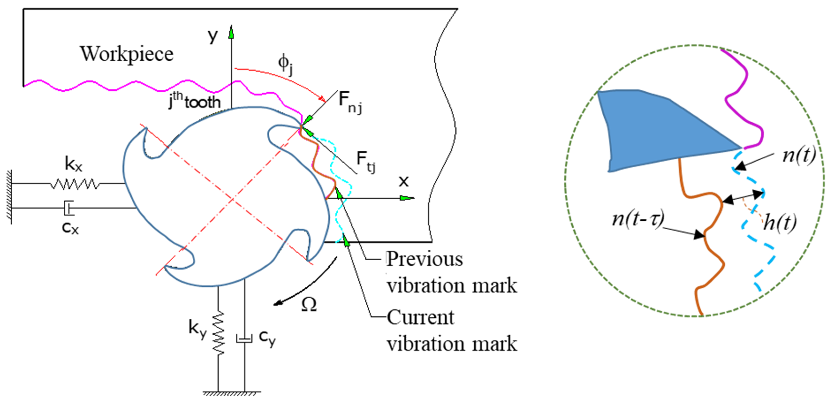
Figure 1 presents a model of the end mill including a milling cutter around two orthogonal degrees of freedom in the feed direction (x) and the normal direction (y). The tool vibration in the x and y directions is projected into the surface normal direction to evaluate the instantaneous chip thickness. The tool vibration in the normal direction is denoted by n.
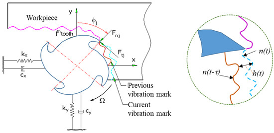
Figure 1.
Dynamic cutting force model of the milling process.
The dynamic displacements x and y are caused when the cutting force excites the structure in those two directions. Therefore, the instantaneous chip thickness for the ith disk element, the jth tooth, and the kth angular position is rewritten in Equation (2) [2]:
where is the feed per tooth. The tooth period is . For the end mill, the instantaneous immersion angle, , is determined by considering the lag angle .
The term [n(t − τ) − n(t)] represents the dynamic chip thickness produced owing to vibrations at the present time t and one spindle revolution period prior. The switching function describes the engagement between each tooth and the workpiece in one revolution, as shown in Equation (6).
The instantaneous chip thickness from Equation (2) can also be rewritten using the x- and y-dynamic displacements as:
where are the dynamic displacements of the cutter in the x and y directions, respectively. The inner and outer modulations are represented by and .
Assuming that the milling cutter is approximated as a system with two orthogonal degrees of freedom in the feed direction (x) and the normal direction (y), the cutting force excites the structure in the x and y directions and causes the dynamic displacements x and y. The equations of motion in the x and y directions, including process damping, are expressed in Equation (8). Here, total damping in the model is assumed, including structural damping and process damping:
where .
The damping coefficient in the normal direction and that in the tangential direction are determined as follows:
in which μ presents the coefficient of contact friction between the flank face and the machined surface. The contact friction coefficients can be determined based on the workpiece and tool material.
Furthermore, the equations of dynamic forces can be converted to (x, y) coordinates in matrix form:
where b is the axial depth of the cut, Kt is the tangential cutting force coefficient, and matrix [A] is the directional coefficients relating the dynamic displacements to the dynamic cutting forces. These directional dynamic force coefficients are calculated via Equations (11)–(14).
Because the matrix can be expressed as a function of time , the term can then be expanded into a Fourier series with Fourier coefficients calculated via Equation (15).
The higher-order terms of the Fourier series are neglected. Then, the dynamic cutting force becomes:
The vibration response in the frequency domain can be represented as Equation (19).
where and are direct transfer functions in the x and y directions. The characteristic equation can be written as in Equation (20).
This results in a quadratic equation, as shown in Equation (23).
The limiting chip width or critical depth of the cut is evaluated from the real and imaginary parts of the eigenvalue , and its relationship with is expressed by Equation (24).
The phase shift between subsequent tooth passages, tooth passing periods, and spindle speeds vs. blim is determined as shown in Equations (25)–(27).
The stability lobe diagram is generated by plotting spindle speeds vs. two limiting chip width values for each chatter frequency.
3. Equilibrium Optimizer Approach
This paper proposes the use of the EO as a recent optimization algorithm that requires few adjustable parameters. Furthermore, cooperation between multiple agents is the focus in EO to improve the exploration manner, supporting global search and avoiding the issue of entrapment in a particular local optimum [52]. Equilibrium Optimizer is a physics-based algorithm that imitates the dynamic mass stabilization behavior within the control volume. The concentration of nonreactive constituents is described as a function of various source and sink dynamics based on the mass balance formulation. The generic mass stabilization is formulated based on a first-order differential equation to describe the variation in the dynamic system due to the mass entering and mass leaving as follows:
where V is the control volume, C is the concentration, F is the flow rate, Ceq is the concentration of the equilibrium state, and G is the generation rate of mass.
The EO algorithm consists of different stages to find the best solutions, and it is defined as follows.
Stage 1: Initialization
The EO starts the initial populations randomly, similarly to other population-based metaheuristics. In this stage, the initial concentrations of each particle are determined randomly within the limits of the system gains as follows:
where Cmin is the minimum concentrations, Cmax is the maximum concentrations, r is random vector within [0, 1], and i is the population index.
After the determination of the concentration of each particle, the fitness function of the optimization problem is evaluated for each particle. Then, the fitness values are sorted to clarify the equilibrium candidates. In the EO algorithm, the four best particles and the mean of these candidates are chosen to represent the equilibrium pool in order to enhance exploration and exploitation behaviors.
Stage 2: Equilibrium pool construction
In this stage, the equilibrium pool is constructed based on the best four particles and their average from the above stage as follows:
Each particle within the population updates its concentration during the iteration’s scope based on each candidate in the selected equilibrium pool with the same probability. In addition, each particle utilizes the same number of updates within the updating process from all of the candidate solutions until the end of the optimization process.
Stage 3: Balancing exploration and exploitation
Obtaining a balance between exploration and exploitation is an essential procedure in optimization problems. The EO algorithm utilizes the exponential term ‘E’ to provide a proper balance between exploration and exploitation. This exponential term ‘E’ is defined as follows:
where is a random factor within [0, 1], while the factors t and t0 are defined as follows:
We substitute t and t0 into Equation (43); then, the exponential term ‘E’ can be described as:
The factors a1 and a2 control the behavior of the exponential term, leading to balance in the exploration and exploitation of the EO algorithm. The term controls the direction of exploration and exploitation within the optimization process.
Stage 4: Convergence to the optimal global solution
In this stage, convergence to the optimal global solution is carried out by utilizing an exponential generation rate factor that is described as follows:
where G0 is the initial value of the generation rate factor and is defined as:
Here, is a controlling factor for the generation rate and is utilized to adjust the exploitation and exploration of each particle as follows:
where r1 and r2 are uniformly distributed random numbers in [0, 1], while is a probability factor. The above stages are performed every iteration to find the best solutions until the stopping criteria are achieved and the best solution for the optimization problem is identified.
4. Results and Discussion
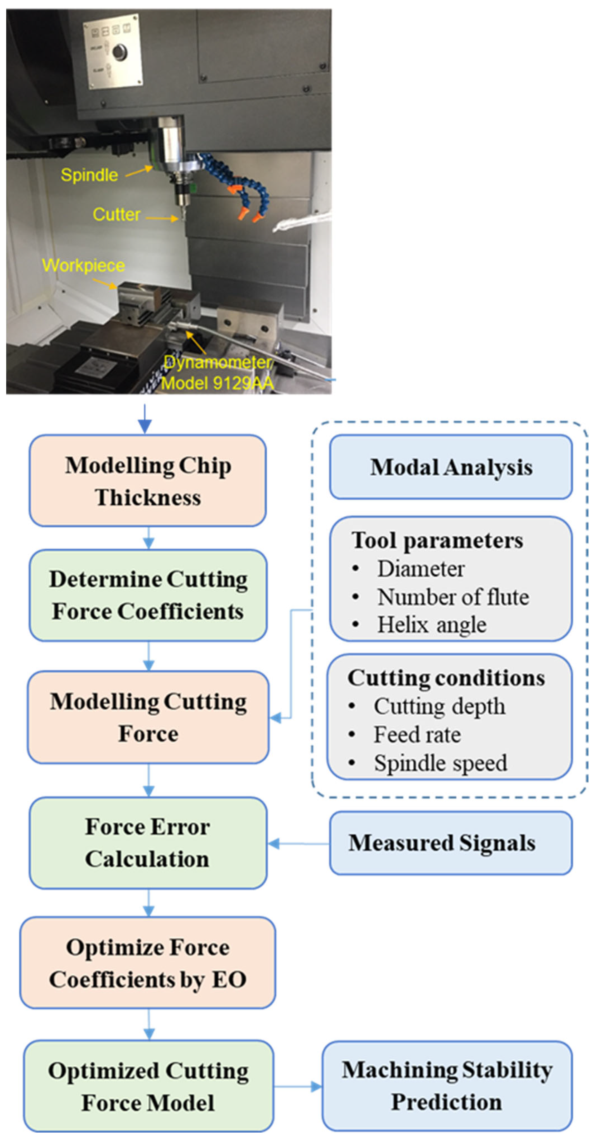
A series of experiments were conducted on a three-axis CNC milling machine (with a Heidenhain TNC620 controller) to determine the specific cutting force coefficients and cutting force angle for the milling force model. The workpiece was a block of Al6061-T6, which is commonly utilized in the automobile and aerospace industries because of its high strength-to-weight ratio. An end mill cutter with a diameter of 12 mm, helix angle of 26°, and two flutes was used. Besides this, the tooth-to-tooth radius error was 6 lm, and the cutting force signals were measured by a Kistler dynamometer mounted between the workpiece and workbench. In this study, lot milling tests were conducted with start cutting angle ϕs = 0 and existing cutting angle ϕe = 180°. The average cutting force in the x and y directions, in this case, is described in Equations (38) and (39).
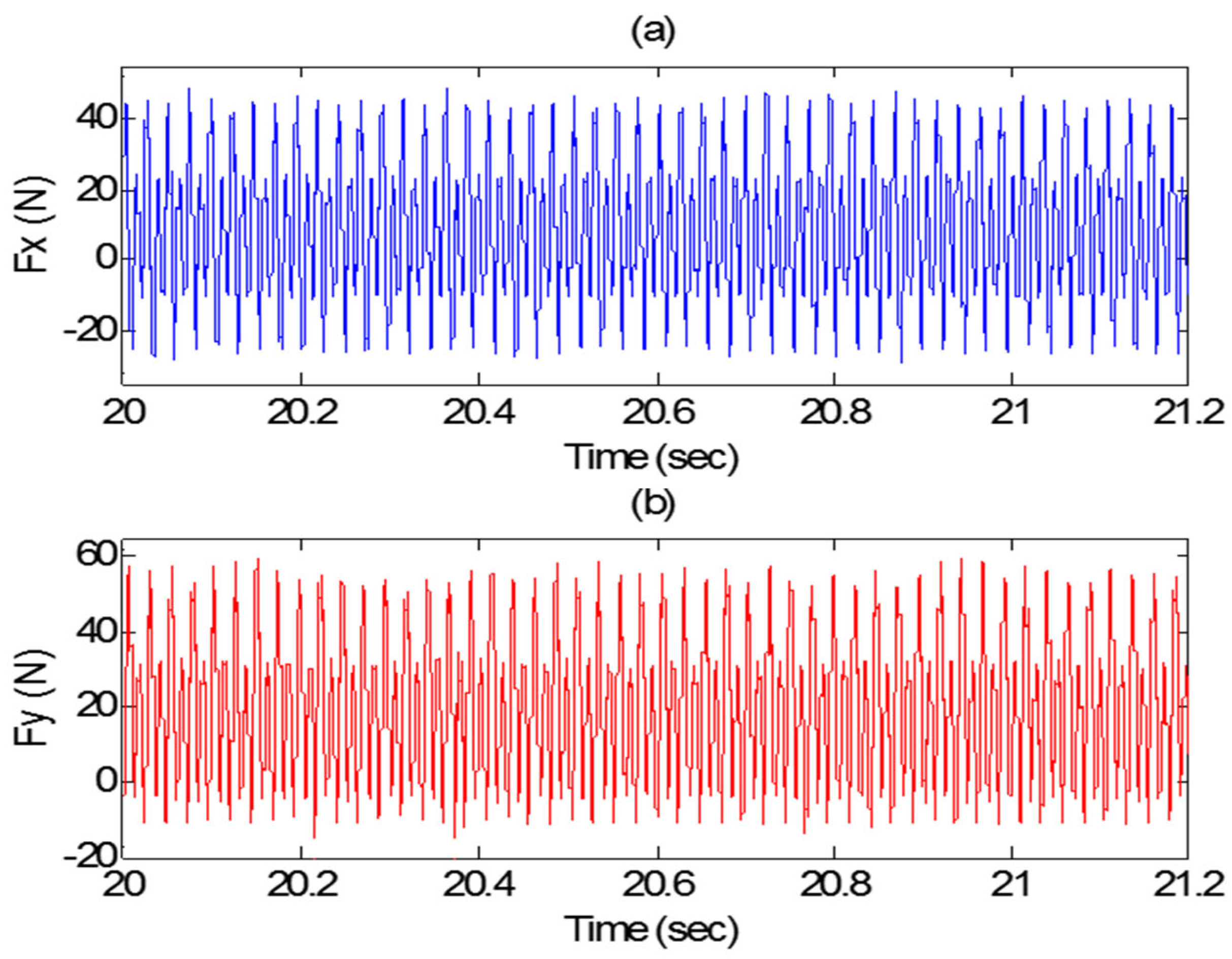
Six slot milling tests corresponding to different feed rates were conducted to achieve average cutting force in the x and y directions. The experimental parameters are provided in Table 1. Figure 2 shows the measured cutting forced signal at a spindle speed of 2500 rpm, cut axial depth of 1 mm, and feed rate of 0.03 mm/tooth in the (a) x-direction and (b) y-direction.

Table 1.
Cutting parameters for cutting force coefficients.
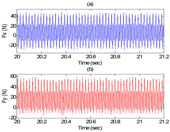
Figure 2.
Measured cutting force signal at a feed rate of 0.03 mm/tooth in the (a) x-direction and (b) y-direction.
The linear regression method summarized by Schmitz [23] was then utilized to determine the four unknown cutting force coefficients in Equations (38) and (39). Those values can be obtained by Equations (40) and (41):
where are the radial and tangential cutting coefficients, respectively, and are the radial and tangential edge coefficients, respectively.
The results of linear regression are shown in Figure 3. The four unknown cutting force coefficients are presented in Table 2. The specific cutting force coefficient and cutting force angle were then calculated following Equation (46).
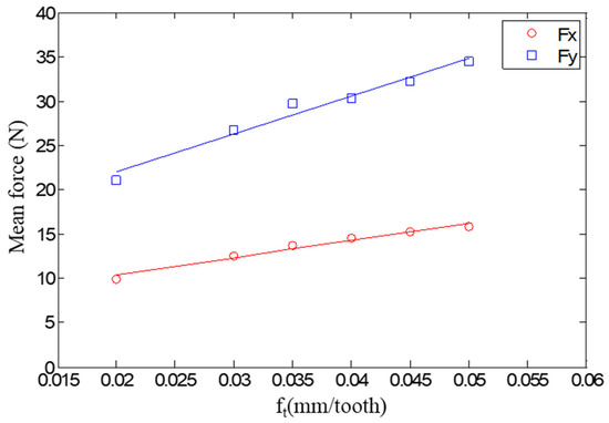
Figure 3.
Relationship between feed per tooth and cutting force.
Table 2.
Specific cutting force coefficients.
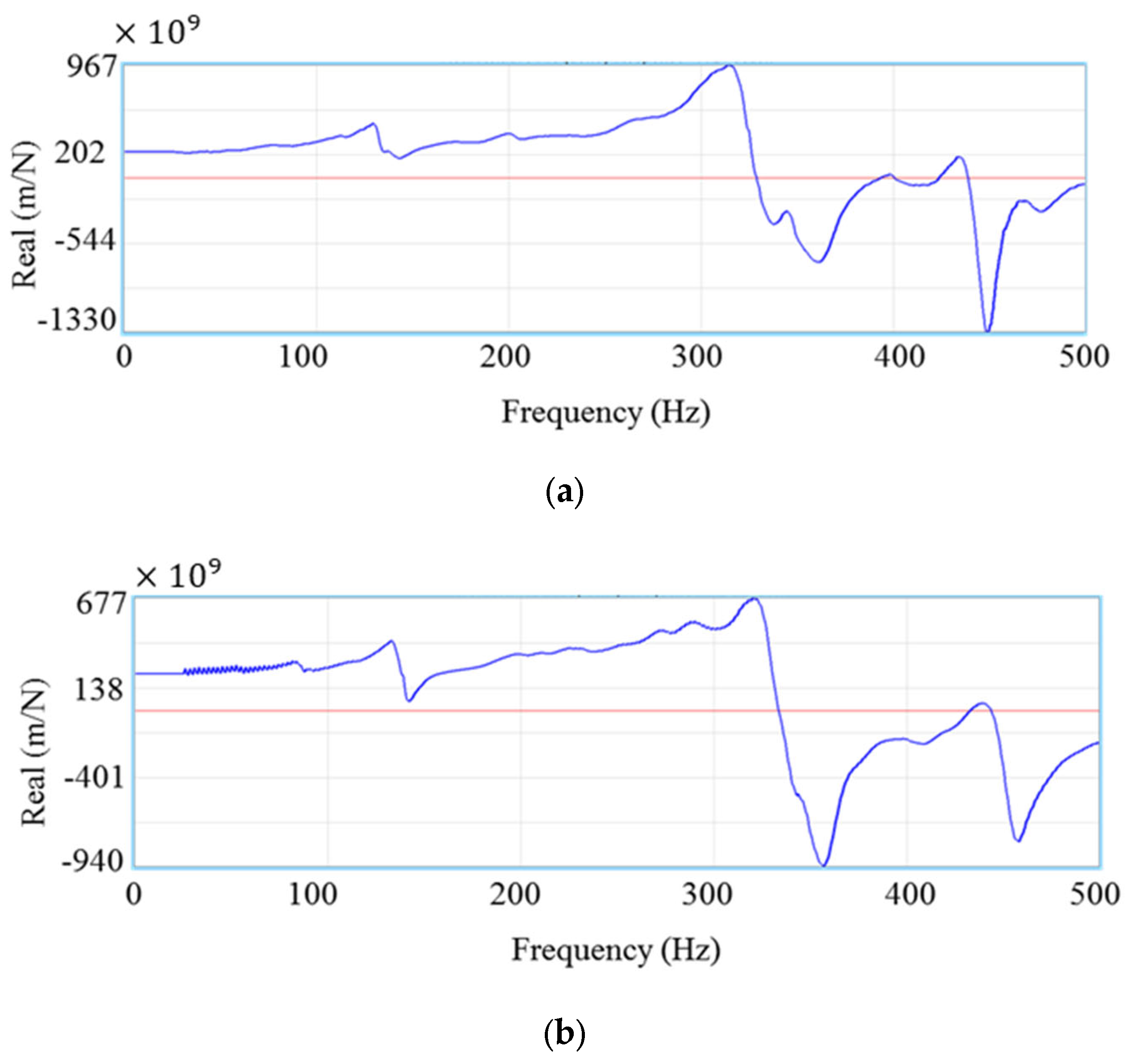
Once the FRFs in the x and y directions were measured, a model was defined by performing a modal fit to the measured data. To identify the modal parameters, the fitting approach was a peak-picking method wherein we used the real and imaginary parts of the system FRFs. This work was done on TXFTM software, and the model fit results are shown in Figure 4a,b in which six modes were selected in both the x and y directions.
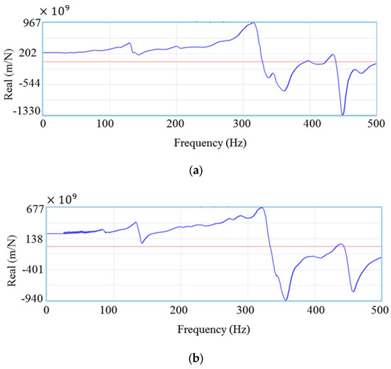
Figure 4.
Relative frequency responses in the (a) x-direction and (b) y-direction.
The peak values of real/imaginary parts were selected, and the corresponding values of frequencies in the x and y directions were applied. Consequently, the model parameters were calculated by using Equations (47)–(49).
Figure 5 illustrates the procedure for optimization of dynamic cutting force coefficients for the end-milling process based on the EO algorithm. The first step was to determine the modal parameters via modal analysis, then the instantaneous chip thickness was calculated using Equation (2). The dynamic cutting force coefficients were generated by the linear regression method. The proposed dynamic cutting force model of milling was used to estimate the cutting forces. Finally, the residual cutting force between the prediction and the actual cutting force was considered as an objective function for optimizing the cutting force coefficients using the EO approach. The boundary of the parameters was adjusted as lower bound = [600 × 106 50 10 × 103 5 × 10³ 1 × 10³] and upper bound = [1000 × 106 90 50 × 103 30 × 103 20 × 103]. As a result, the optimum set of specific cutting force coefficients by the EO method was obtained, as presented in Table 3.
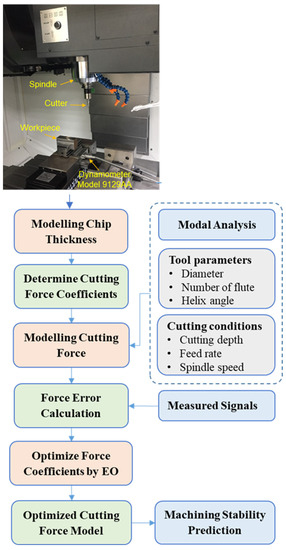
Figure 5.
Procedure for optimization of dynamic cutting force coefficients for the end-milling process.
Table 3.
The optimum set of specific cutting force coefficients by EO.
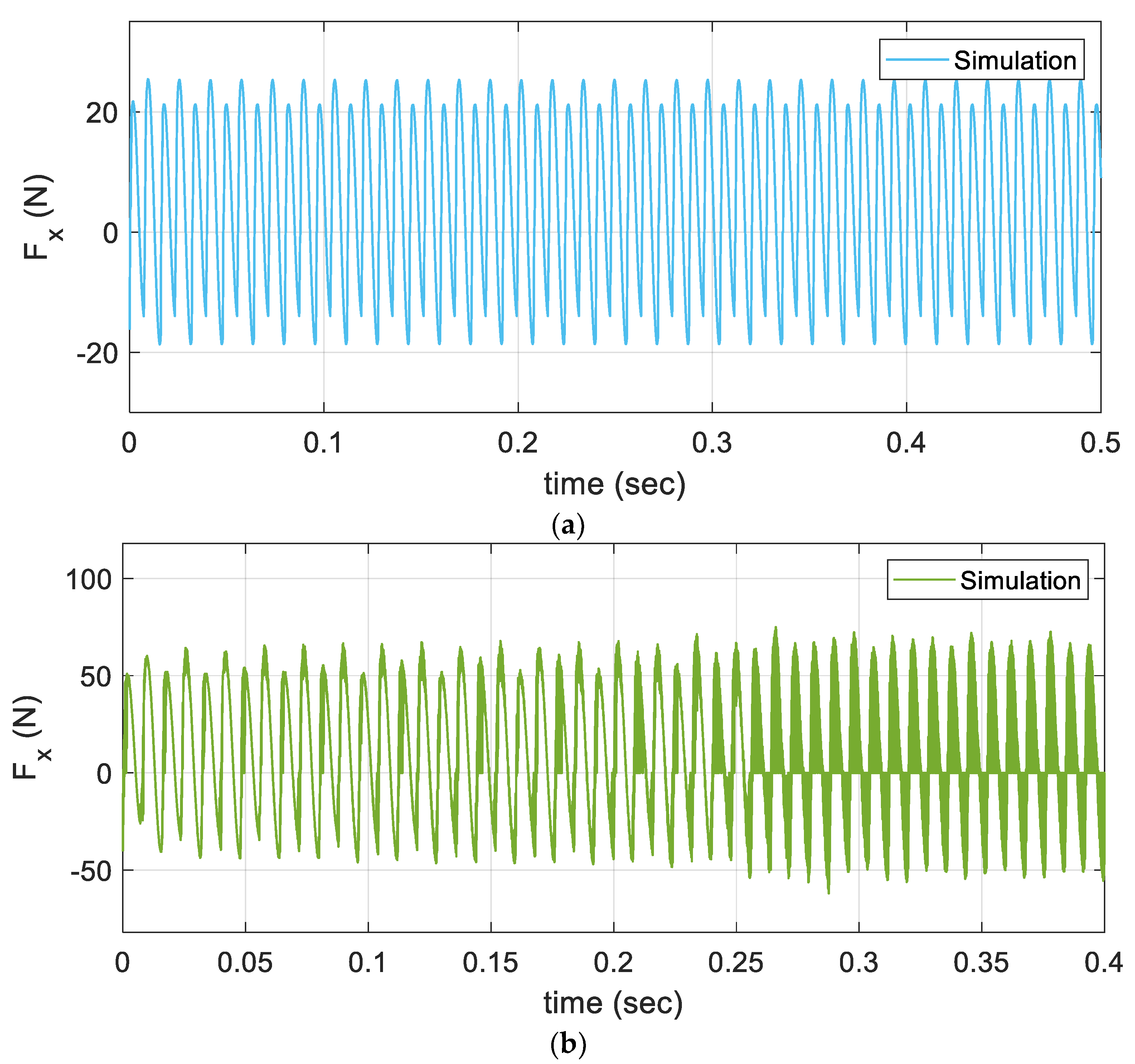
The simulation cutting forces under various cutting conditions are shown in Figure 6, in which the stable cutting condition in Figure 6a indicates that the cutting force behavior is repetitive from one to the next cutting revolution. On the other hand, in Figure 6b, the repetitive behavior of the cutting force does not remain from one to the next cutting revolution of the cutter; instead, the magnitude of the cutting force eventually increases during the cutting.
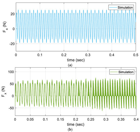
Figure 6.
Simulation of cutting force under different cutting conditions: (a) stable cutting: 3750 rpm spindle and 0.4 mm cut depth; (b) unstable cutting: 3750 rpm spindle and 1.4 mm cut depth.
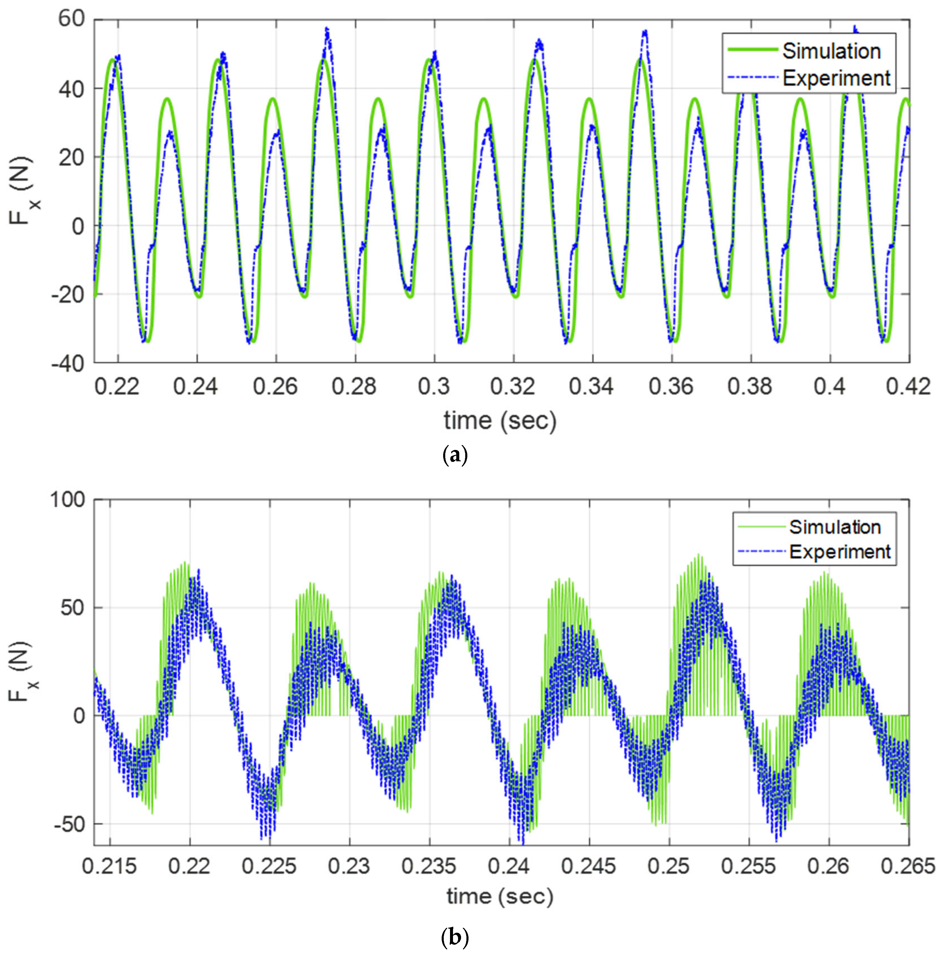
Figure 7 shows the performance of the cutting force model when experimentally validated by the measured cutting force. A comparison between the simulated and experimental results for both stable and unstable cutting conditions is presented in Figure 7a,b, respectively. The simulated results coincide with the measured cutting forces. Moreover, this study provides a new solution for the tuning of the force factors of the milling process based on an intelligent algorithm named EO instead of trial-and-error methods. The EO algorithm finds the best force factors based on the minimization of the integral square error (ISE), defined as follows:
where
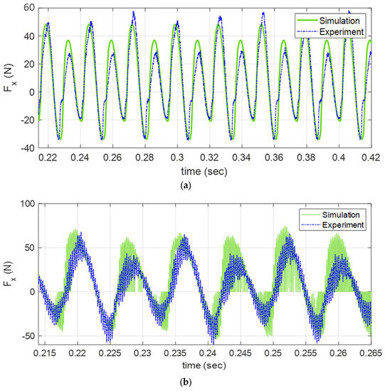
Figure 7.
Experimental validation of the cutting force model: (a) stable cutting: 2250 rpm spindle and 1.4 mm cut depth; (b) unstable cutting: 3750 rpm spindle and 1.4 mm cut depth.
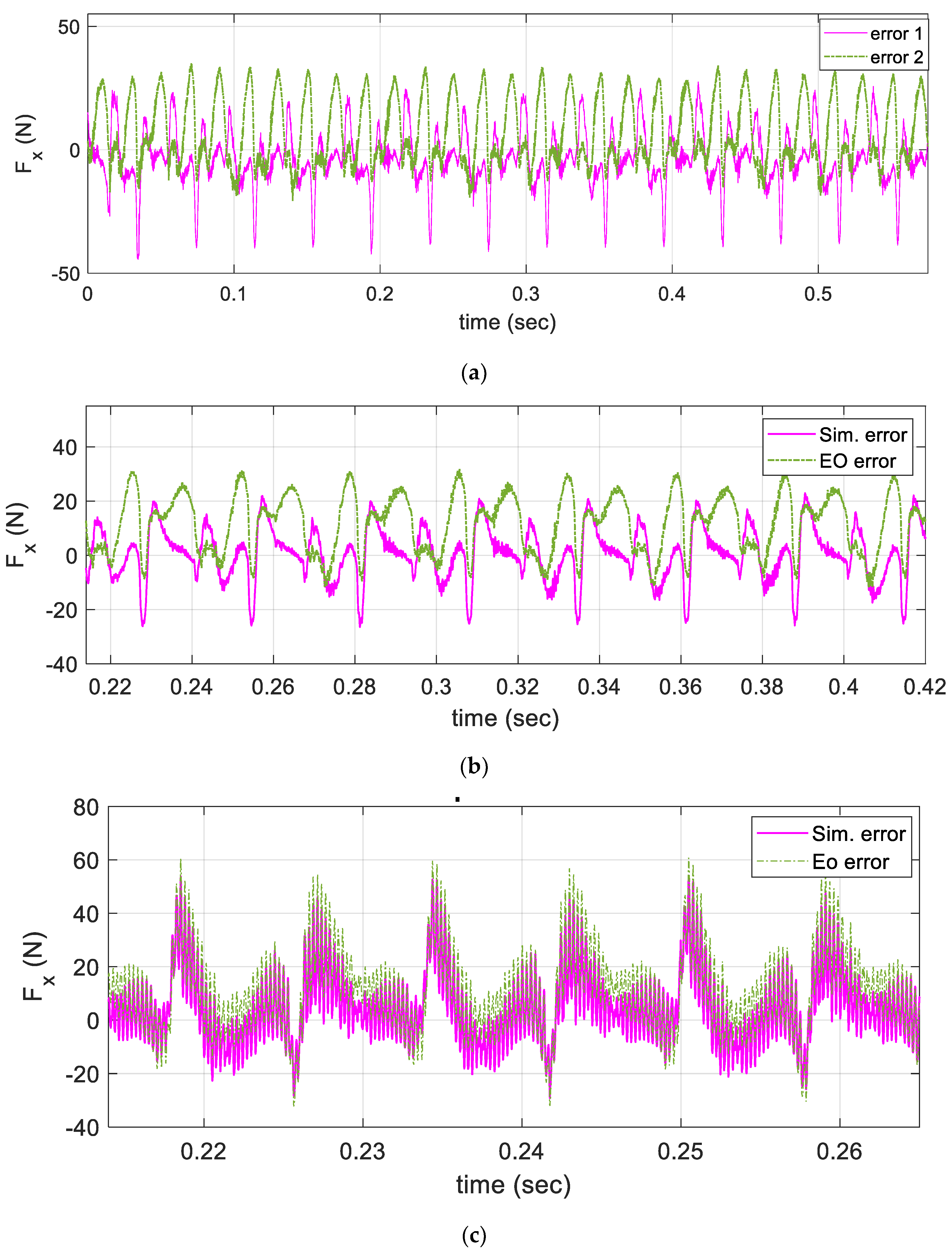
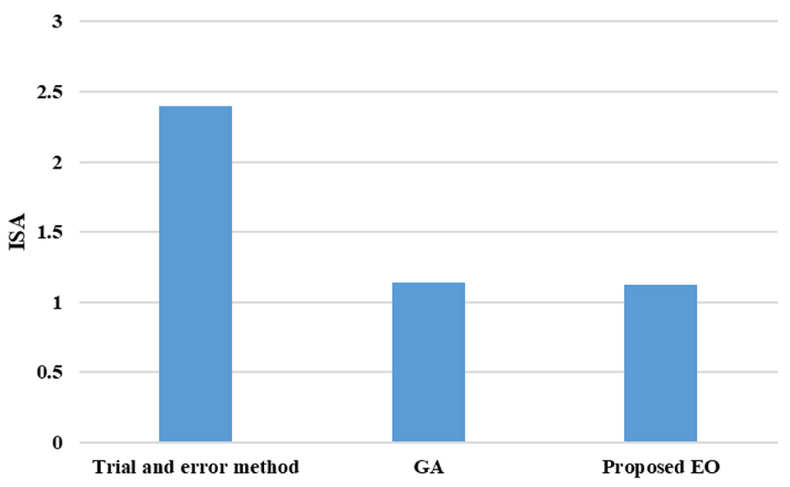
As the result, the errors of the cutting forces of the proposed dynamic cutting force model with and without the EO method are illustrated in Figure 8. The figure shows that the performance of the cutting force model is improved when applying the EO algorithm to correct the specific cutting force coefficients. The errors between simulated and measured cutting forces are significantly reduced with the EO method in both stable and unstable cutting conditions. Moreover, the integral square error values based on trial and error, GA, and the proposed EO method are shown in Figure 9 and Table 4. It is clear that the proposed EO has a minimum ISE of around 1.12, while the GA has an ISE of around 1.14 and the trial-and-error method has an ISE of around 2.4. The ISE values of the cutting force model are significantly decreased when correcting the cutting force coefficients by the EO algorithm.
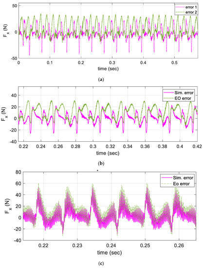
Figure 8.
Residual values of the proposed dynamic cutting force model with and without the EO method: (a) stable cutting: 1500 rpm spindle and 1.4 mm cut depth; (b) stable cutting: 2250 rpm spindle and 1.4 mm cut depth; (c) unstable cutting: 3750 rpm spindle and 1.4 mm cut depth.

Figure 9.
Integral square error values from simulation with and without the EO method.
Table 4.
ISE values in the case of the proposed EO and different techniques in literature.
5. Conclusions
During the milling process, the engagement between the tool and the workpiece relatively oscillates and affects the cutting depth. This might include both cutting force vibration and cutting chatter vibration and creates difficulty in modeling the cutting force. In this study, we proposed a dynamic cutting force model of the milling process, in which the modal parameters were determined via impact testing and modal analysis. The dynamic cutting force coefficients were generated by the linear regression method. The proposed dynamic cutting force model of milling was used to estimate the cutting forces. Finally, the square error of the residual cutting force between the prediction and the actual cutting force was considered as an objective function to optimize the cutting force coefficients using the EO approach. The linear regression method was firstly used to determine the specific cutting force coefficients, and then the EO algorithm was adopted to optimize the set of specific cutting force coefficients based on minimization of the integral square error between the simulated and measured cutting forces. The performance of the proposed force model was experimentally validated under various cutting conditions. The results indicate that the cutting force model was significantly improved by applying the EO algorithm to correct the specific cutting force coefficients. The proposed EO had a minimum ISE of around 1.12, while the GA had an ISE of around 1.14 and the trial-and-error method had an ISE of around 2.4. The errors between the simulated and measured cutting forces were also significantly reduced by the EO method under both stable and unstable cutting conditions.
Author Contributions
Conceptualization, M.E. and M.-Q.T.; Data curation, M.E. and M.-Q.T.; Formal analysis, M.E., M.-Q.T. and V.Q.V.; Funding acquisition, F.A. and S.S.M.G.; Investigation, M.-Q.T., V.Q.V., F.A. and S.S.M.G.; Methodology, M.E. and M.-Q.T.; Project administration, F.A.; Resources, M.E. and F.A.; Software, M.-Q.T.; Supervision, M.E. and S.S.M.G.; Validation, V.Q.V., F.A. and S.S.M.G.; Visualization, V.Q.V., F.A. and S.S.M.G.; Writing—original draft, M.E. and M.-Q.T.; Writing—review and editing, V.Q.V., F.A. and S.S.M.G. All authors have read and agreed to the published version of the manuscript.
Funding
This work was supported by Taif University Researchers Supporting Project number (TURSP-2020/97), Taif University, Taif, Saudi Arabia and in part by the Ministry of Science and Technology (MOST) of Taiwan (grant numbers: MOST 110-2222-E-011-002- and MOST 110-2222-E-011-013-).
Institutional Review Board Statement
Not applicable.
Informed Consent Statement
Not applicable.
Data Availability Statement
Not applicable.
Acknowledgments
The authors would like to thank Taif University Researchers Supporting Project number (TURSP-2020/97), Taif University, Taif, Saudi Arabia for supporting this work.
Conflicts of Interest
The authors declare no conflict of interest.
References
- Pereira, R.B.D.; Brandão, L.C.; de Paiva, A.P.; Ferreira, J.R.; Davim, J.P. A review of helical milling process. Int. J. Mach. Tools Manuf. 2017, 120, 27–48. [Google Scholar] [CrossRef]
- Altintas, Y. Manufacturing Automation: Metal Cutting Mechanics, Machine Tool Vibrations, and CNC Design, 2nd ed.; Cambridge University Press: Cambridge, UK, 2012. [Google Scholar]
- Taner, T.L.; Ömer, Ö.; Erhan, B. Generalized cutting force model in multi-Axis milling using a new engagement boundary determination approach. Int. J. Adv. Manuf. Technol. 2015, 77, 341–355. [Google Scholar] [CrossRef]
- Chung, C.; Tran, M.-Q.; Liu, M.-K. Estimation of Process Damping Coefficient Using Dynamic Cutting Force Model. Int. J. Precis. Eng. Manuf. 2020, 21, 623–632. [Google Scholar] [CrossRef]
- Yue, C.; Gao, H.; Liu, X.; Liang, S.Y.; Wang, L. A review of chatter vibration research in milling. Chin. J. Aeronaut. 2019, 32, 215–242. [Google Scholar] [CrossRef]
- Moon, F.C.; Kalmár-Nagy, T. Nonlinear Models for Complex Dynamics in Cutting Materials. Philos. Trans. Math. Phys. Eng. Sci. 2001, 359, 695–711. [Google Scholar] [CrossRef]
- Kasahara, N.; Sato, H.; Tani, Y. Phase Characteristics of Self-Excited Chatter in Cutting. J. Eng. Ind. 1992, 114, 393–399. [Google Scholar] [CrossRef]
- Munoa, J.; Beudaert, X.; Dombovari, Z.; Altintas, Y.; Budak, E.; Brecher, C.; Stepan, G. Chatter suppression techniques in metal cutting. CIRP Ann. 2016, 65, 785–808. [Google Scholar] [CrossRef]
- Zengxi, P.; Hui, Z. Analysis and suppression of chatter in robotic machining process. In Proceedings of the 2007 International Conference on Control, Automation and Systems, Seoul, Korea, 17–20 October 2007; pp. 595–600. [Google Scholar] [CrossRef]
- Ding, L.; Sun, Y.; Xiong, Z. Active Chatter Suppression in Turning by Simultaneous Adjustment of Amplitude and Frequency of Spindle Speed Variation. J. Manuf. Sci. Eng. 2019, 142, 021004. [Google Scholar] [CrossRef]
- Altintas, Y.; Stepan, G.; Budak, E.; Schmitz, T.; Kilic, Z.M. Chatter Stability of Machining Operations. J. Manuf. Sci. Eng. 2020, 142, 110801. [Google Scholar] [CrossRef]
- Tran, M.-Q.; Liu, M.-K.; Elsisi, M. Effective multi-Sensor data fusion for chatter detection in milling process. ISA Trans. 2021, 125, 514–527. [Google Scholar] [CrossRef]
- Mohammadi, Y.; Ahmadi, K. Frequency domain analysis of regenerative chatter in machine tools with Linear Time Periodic dynamics. Mech. Syst. Signal Process. 2019, 120, 378–391. [Google Scholar] [CrossRef]
- Mou, W.; Zhu, S.; Jiang, Z.; Song, G. Vibration signal-Based chatter identification for milling of thin-Walled structure. Chin. J. Aeronaut. 2022, 35, 204–214. [Google Scholar] [CrossRef]
- Perrelli, M.; Cosco, F.; Gagliardi, F.; Mundo, D. In-Process Chatter Detection Using Signal Analysis in Frequency and Time-Frequency Domain. Machines 2022, 10, 24. [Google Scholar] [CrossRef]
- Tran, M.-Q.; Elsisi, M.; Liu, M.-K. Effective feature selection with fuzzy entropy and similarity classifier for chatter vibration diagnosis. Measurement 2021, 184, 109962. [Google Scholar] [CrossRef]
- Yoon, M.C.; Chin, D.H. Cutting force monitoring in the endmilling operation for chatter detection. Proc. Inst. Mech. Eng. Part B J. Eng. Manuf. 2005, 219, 455–465. [Google Scholar] [CrossRef]
- Sun, Y.; Jiang, S. Predictive modeling of chatter stability considering force-Induced deformation effect in milling thin-Walled parts. Int. J. Mach. Tools Manuf. 2018, 135, 38–52. [Google Scholar] [CrossRef]
- Zhang, X.; Zhang, J.; Pang, B.; Zhao, W. An accurate prediction method of cutting forces in 5-Axis flank milling of sculptured surface. Int. J. Mach. Tools Manuf. 2016, 104, 26–36. [Google Scholar] [CrossRef]
- Ji, Y.; Bi, Q.; Zhang, S.; Wang, Y. A new receptance coupling substructure analysis methodology to predict tool tip dynamics. Int. J. Mach. Tools Manuf. 2018, 126, 18–26. [Google Scholar] [CrossRef]
- Zhang, J.; Li, J.; Xie, Z.; Du, C.; Gui, L.; Zhao, W. Rapid dynamics prediction of tool point for bi-Rotary head five-Axis machine tool. Precis. Eng. 2017, 48, 203–215. [Google Scholar] [CrossRef]
- Liu, M.-K.; Tran, M.-Q.; Chung, C.; Qui, Y.-W. Hybrid model- and signal-Based chatter detection in the milling process. J. Mech. Sci. Technol. 2020, 34, 1–10. [Google Scholar] [CrossRef]
- Smith, K.S.; Schmitz, T.L. Machining Dynamics: Frequency Response to Improved Productivity; Springer International Publishing: Berlin/Heidelberg, Germany, 2008. [Google Scholar]
- Tran, M.-Q.; Liu, M.-K.; Tran, Q.-V. Analysis of Milling Chatter Vibration Based on Force Signal in Time Domain. In Advances in Engineering Research and Application; Sattler, K.-U., Nguyen, D.C., Vu, N.P., Long, B.T., Puta, H., Eds.; Springer International Publishing: Berlin/Heidelberg, Germany, 2021; pp. 192–199. [Google Scholar]
- Liu, M.-K.; Tran, Q.M.; Qui, Y.-W.; Chung, C.-H. Chatter Detection in Milling Process Based on Time-Frequency Analysis. In Proceedings of the ASME 2017 12th International Manufacturing Science and Engineering Conference Collocated with the JSME/ASME 2017 6th International Conference on Materials and Processing, Los Angeles, CA, USA, 4–8 June 2017; Volume 1, p. V001T02A025. [Google Scholar] [CrossRef]
- Liu, C.; Zhu, L.; Ni, C. The chatter identification in end milling based on combining EMD and WPD. Int. J. Adv. Manuf. Technol. 2017, 91, 3339–3348. [Google Scholar] [CrossRef]
- Gao, G.; Wu, B.; Zhang, D.; Luo, M. Mechanistic identification of cutting force coefficients in bull-Nose milling process. Chin. J. Aeronaut. 2013, 26, 823–830. [Google Scholar] [CrossRef]
- Adem, K.A.M.; Fales, R.; El-Gizawy, A.S. Identification of cutting force coefficients for the linear and nonlinear force models in end milling process using average forces and optimization technique methods. Int. J. Adv. Manuf. Technol. 2015, 79, 1671–1687. [Google Scholar] [CrossRef]
- Budak, E.; Altintas, Y.; Armarego, E.J.A. Prediction of Milling Force Coefficients from Orthogonal Cutting Data. J. Manuf. Sci. Eng. 1996, 118, 216–224. [Google Scholar] [CrossRef]
- Chen, X.; Zhang, D.; Wang, Q. Cutting Force Transition Model Considering the Influence of Tool System by Using Standard Test Table. Sensors 2021, 21, 1340. [Google Scholar] [CrossRef] [PubMed]
- Lamikiz, A.; de Lacalle, L.N.L.; Sanchez, J.A.; Bravo, U. Calculation of the specific cutting coefficients and geometrical aspects in sculptured surface machining. Mach. Sci. Technol. 2005, 9, 411–436. [Google Scholar] [CrossRef]
- Elsisi, M.; Ebrahim, M.A. Optimal design of low computational burden model predictive control based on SSDA towards autonomous vehicle under vision dynamics. Int. J. Intell. Syst. 2021, 36, 6968–6987. [Google Scholar] [CrossRef]
- Halim, A.H.; Ismail, I.; Das, S. Performance assessment of the metaheuristic optimization algorithms: An exhaustive review. Artif. Intell. Rev. 2021, 54, 2323–2409. [Google Scholar] [CrossRef]
- Elsisi, M.; Tran, M.Q.; Hasanien, H.M.; Turky, R.A.; Albalawi, F.; Ghoneim, S.S. Robust model predictive control paradigm for automatic voltage regulators against uncertainty based on optimization algorithms. Mathematics 2021, 9, 2885. [Google Scholar] [CrossRef]
- Ding, J.; Xiao, D.; Li, X. Gear fault diagnosis based on genetic mutation particle swarm optimization VMD and probabilistic neural network algorithm. IEEE Access 2020, 8, 18456–18474. [Google Scholar] [CrossRef]
- Seyfipour, N.; Menhaj, M.; Nik, R. A New Optimization Method by Ring Probabilistic Logic Neural Networks. AMIRKABIR 2003, 14, 43–57. [Google Scholar]
- Azizi, A.; Vatankhah Barenji, A.; Hashmipour, M. Optimizing radio frequency identification network planning through ring probabilistic logic neurons. Adv. Mech. Eng. 2016, 8, 1687814016663476. [Google Scholar] [CrossRef]
- Menhaj, M.B.; Seifipour, N. Function optimization by RPLNN. In Proceedings of the 2002 International Joint Conference on Neural Networks, IJCNN’02 (Cat. No. 02CH37290), Honolulu, HI, USA, 12–17 May 2002; Volume 2, pp. 1522–1527. [Google Scholar]
- Qu, M.; Tang, J. Probabilistic logic neural networks for reasoning. arXiv 2019, arXiv:1906.08495. [Google Scholar]
- Guo, X.; Albalawi, F.; Laleg-Kirati, T.-M. Observer-based economic model predictive control for direct contact membrane distillation. Chem. Eng. Res. Des. 2020, 156, 86–99. [Google Scholar] [CrossRef]
- Cao, Y.; Zhang, H.; Li, W.; Zhou, M.; Zhang, Y.; Chaovalitwongse, W.A. Comprehensive learning particle swarm optimization algorithm with local search for multimodal functions. IEEE Trans. Evol. Comput. 2018, 23, 718–731. [Google Scholar] [CrossRef]
- Alanqar, A.; Durand, H.; Albalawi, F.; Christofides, P.D. An economic model predictive control approach to integrated production management and process operation. AIChE J. 2017, 63, 1892–1906. [Google Scholar] [CrossRef]
- Li, W.; Wang, G.G.; Gandomi, A.H. A survey of learning-Based intelligent optimization algorithms. Arch. Comput. Methods Eng. 2021, 28, 3781–3799. [Google Scholar] [CrossRef]
- Albalawi, F.; Durand, H.; Christofides, P.D. Distributed economic model predictive control with Safeness-Index based constraints for nonlinear systems. Syst. Control Lett. 2017, 110, 21–28. [Google Scholar] [CrossRef]
- Sahoo, A.K.; Jeet, S.; Bagal, D.K.; Barua, A.; Pattanaik, A.K.; Behera, N. Parametric optimization of CNC-drilling of Inconel 718 with cryogenically treated drill-Bit using Taguchi-Whale optimization algorithm. Mater. Today Proc. 2022, 50, 1591–1598. [Google Scholar] [CrossRef]
- Huang, X.; He, Z.; Chen, Y.; Xie, S. A Divide-And-Conquer Bat Algorithm with Direction of Mean Best Position for Optimization of Cutting Parameters in CNC Turnings. Comput. Intell. Neurosci. 2022, 2022, 4719266. [Google Scholar] [CrossRef]
- Sun, Y.; Yang, T.; Liu, Z. A whale optimization algorithm based on quadratic interpolation for high-Dimensional global optimization problems. Appl. Soft Comput. 2019, 85, 105744. [Google Scholar] [CrossRef]
- Emami, M.; Nazif, S.; Mousavi, S.F.; Karami, H.; Daccache, A. A hybrid constrained coral reefs optimization algorithm with machine learning for optimizing multi-Reservoir systems operation. J. Environ. Manag. 2021, 286, 112250. [Google Scholar] [CrossRef] [PubMed]
- Houssein, E.H.; Helmy, B.E.D.; Rezk, H.; Nassef, A.M. An enhanced Archimedes optimization algorithm based on Local escaping operator and Orthogonal learning for PEM fuel cell parameter identification. Eng. Appl. Artif. Intell. 2021, 103, 104309. [Google Scholar] [CrossRef]
- Elsheikh, A.H.; Shehabeldeen, T.A.; Zhou, J.; Showaib, E.; Abd Elaziz, M. Prediction of laser cutting parameters for polymethylmethacrylate sheets using random vector functional link network integrated with equilibrium optimizer. J. Intell. Manuf. 2020, 32, 1377–1388. [Google Scholar] [CrossRef]
- Yu, H.; Yang, B.; Wang, S.; Wang, Y.; Wang, S.; Wang, Z.; Wang, Z. An effective multi-Part dedicatedflow-Line reconfiguration model considering the optimal selection of machining process path and machines. Proc. Inst. Mech. Eng. Part B J. Eng. Manuf. 2022, 09544054221100873. [Google Scholar] [CrossRef]
- Faramarzi, A.; Heidarinejad, M.; Stephens, B.; Mirjalili, S. Equilibrium optimizer: A novel optimization algorithm. Knowl.-Based Syst. 2020, 191, 105190. [Google Scholar] [CrossRef]
- Gao, Y.; Zhou, Y.; Luo, Q. An efficient binary equilibrium optimizer algorithm for feature selection. IEEE Access 2020, 8, 140936–140963. [Google Scholar] [CrossRef]
- Houssein, E.H.; Dirar, M.; Abualigah, L.; Mohamed, W.M. An efficient equilibrium optimizer with support vector regression for stock market prediction. Neural Comput. Appl. 2022, 34, 3165–3200. [Google Scholar] [CrossRef]

Publisher’s Note: MDPI stays neutral with regard to jurisdictional claims in published maps and institutional affiliations. |
© 2022 by the authors. Licensee MDPI, Basel, Switzerland. This article is an open access article distributed under the terms and conditions of the Creative Commons Attribution (CC BY) license (https://creativecommons.org/licenses/by/4.0/).