
CLTSA: A Novel Tunicate Swarm Algorithm Based on Chaotic-Lévy Flight Strategy for Solving Optimization Problems


Abstract
:1. Introduction
2. Related Work
3. The Proposed CLTSA
3.1. TSA
- Avoiding clashes between each search agent.
- Each agent is guaranteed to move in the direction of the optimal individual.
- Make the search agents converge to the region near the optimal individual.
3.1.1. Avoiding Clashes between Each Search Agent
3.1.2. Move in the Direction of the Optimal Individual
3.1.3. Make the Search Agents Converge to the Optimal Individual
3.1.4. Swarm Behavior
3.2. Lévy Flight
3.3. Chaotic Maps
- Chebyshev map
- Circle map
- Gauss map
- Iterative chaotic map with infinite collapses (ICMIC)
- Logistic map
- Sine map
- Singer map
- Sinusoidal map
- Tent map
3.4. Chaotic-Lévy Flight TSA
| Algorithm 1: Algorithm CLTSA |
| 1: procedure CLTSA |
| 2: Initialize the original population X and the randomly |
| 3: Initialize the parameters and maximum number of iterations T 4: set 5: Calculate fitness of each individual, and choose the best candidate solution as 6: while (t < T) do 7: for do /* Jet propulsion behavior */ 8: 9: Equation (4) 10: Equation (3) 11: Equation (2) 12: Equation (1) 13: Equation (5) 14: Equation (17)–(25) 15: Equation (13)–(16) /* Swarm behavior */ 16: if 17: if 18: Equation (6) 19: else 20: 21: end if 22: else 23: if 24: Equation (26) 25: else 26: 27: end if 28: Equation (7) 29: end for 30: Calculate fitness of each individual, and choose the best solution as 31: 32: end while 33: return 34: end procedure |
3.5. Complexity Analysis of CLTSA
3.5.1. Time Complexity
3.5.2. Space Complexity
4. Experimental Results and Analysis
4.1. Benchmark Test Functions
- Unimodal benchmark functions: The detailed information of the unimodal functions test set is listed in Table 2, and their mathematical expressions are shown in Table A1 in Appendix A [11].
- Multimodal benchmark functions: The detailed information of the test set which is composed of 14 multimodal benchmark functions is listed in Table 3, and their mathematical expressions are shown in Table A2 in Appendix A [11].
4.2. Comparison of Chaotic Maps
4.3. Parameter Settings of TLTSA and Other Algorithms
4.4. Results and Analysis
4.4.1. Experimental Data Analysis
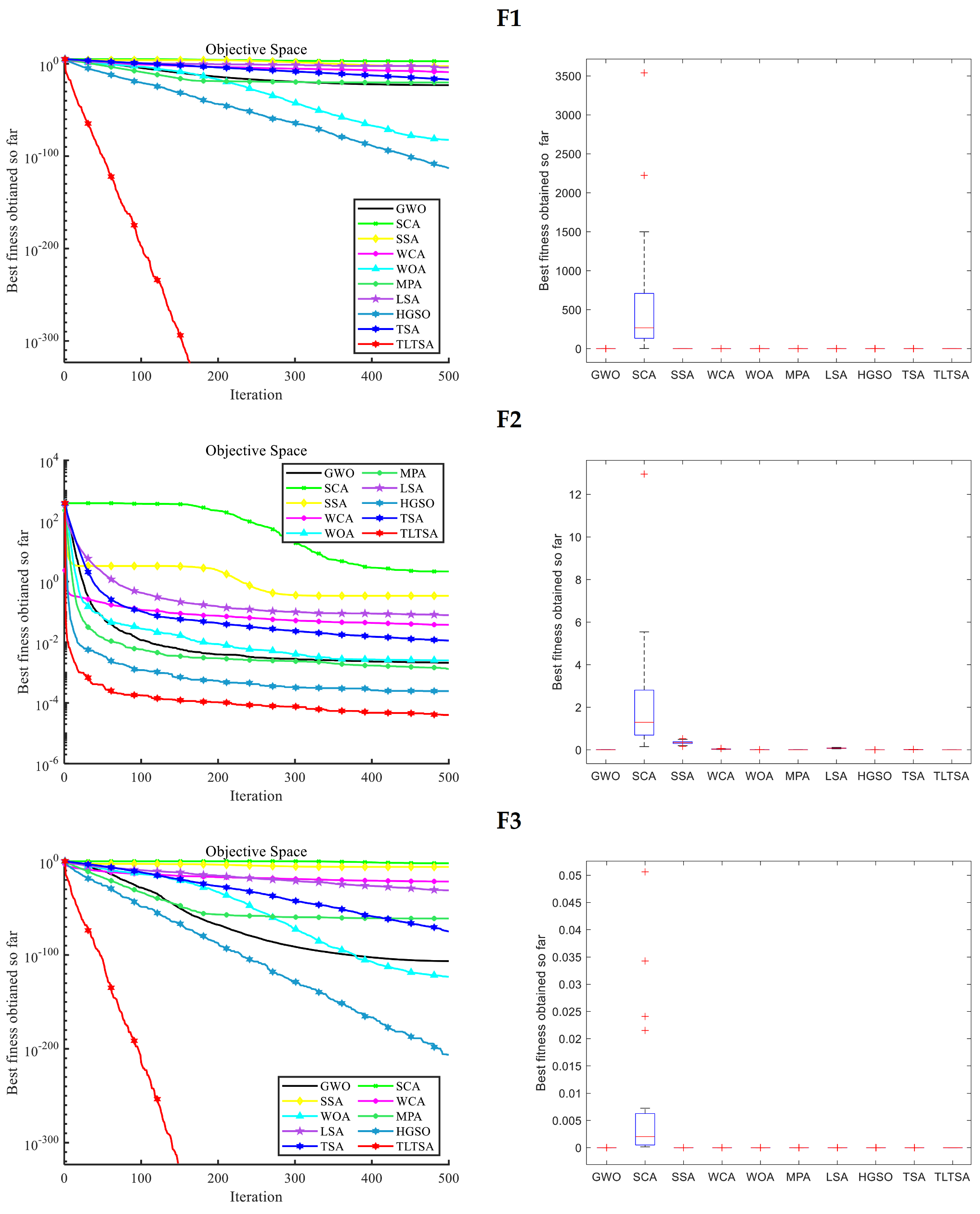
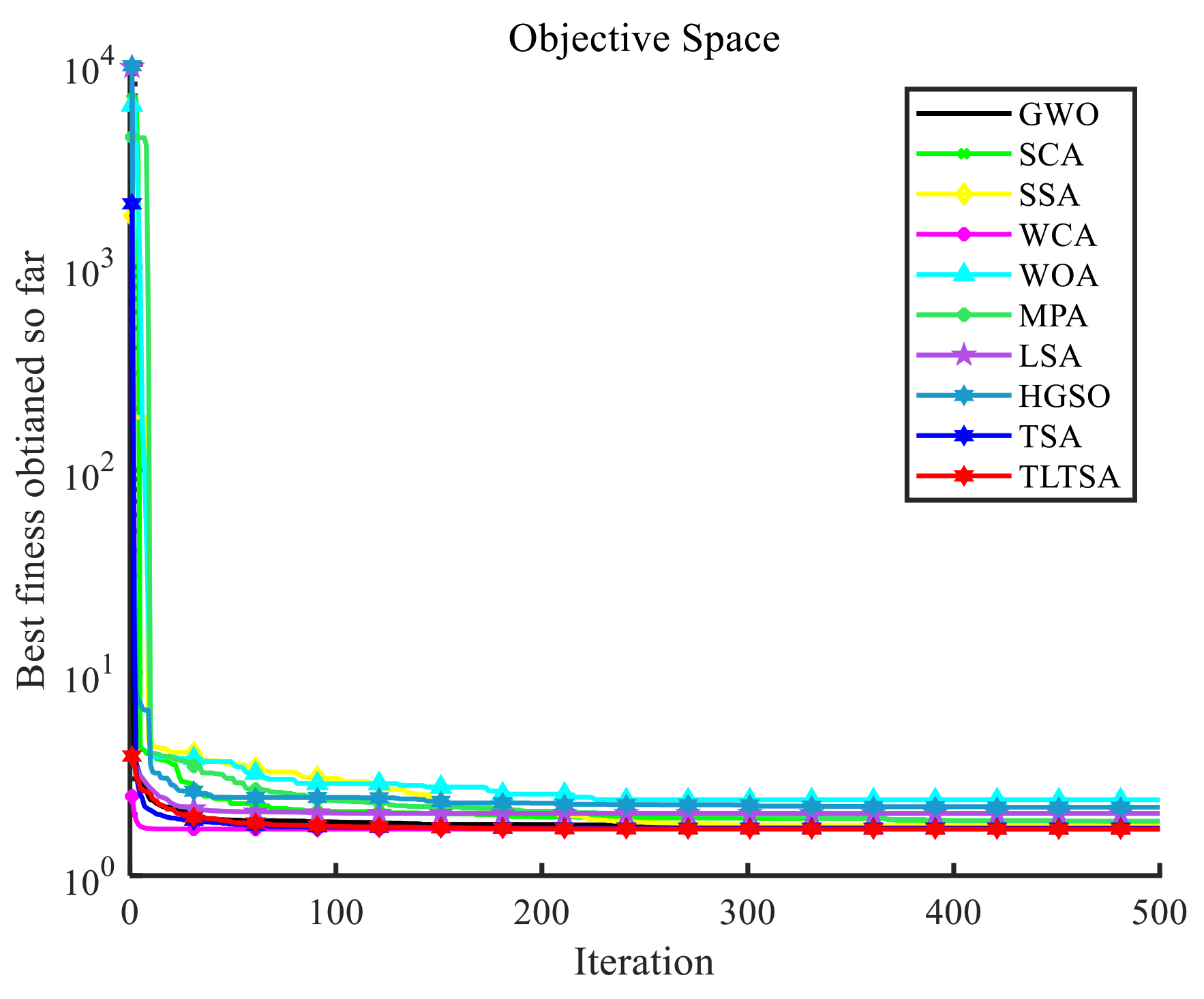
4.4.2. Convergence Curve and Boxplot Analysis
4.4.3. Statistical Test
5. TLTSA for Complex Problems in the Engineering Field
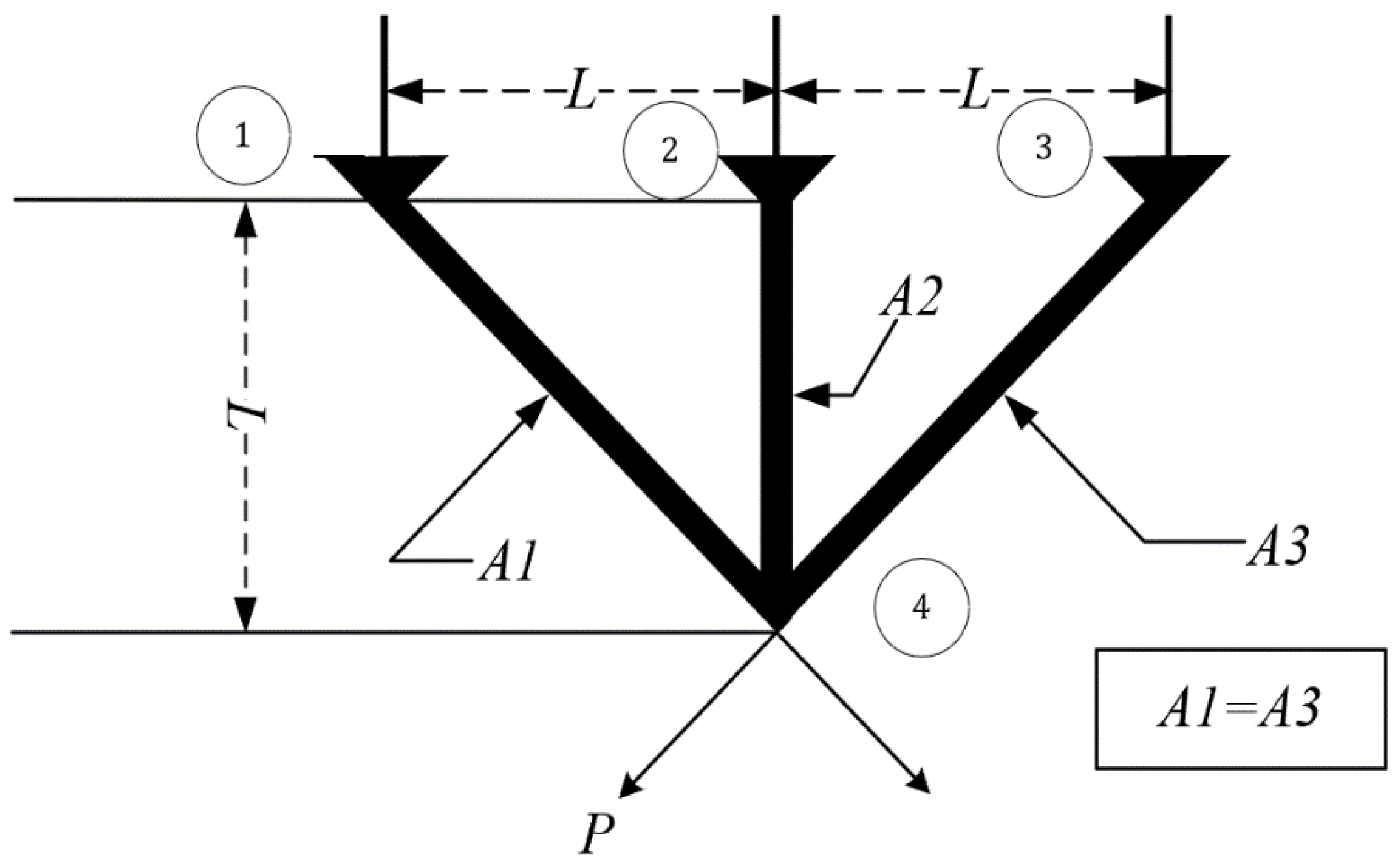
5.1. Three-Bar Truss Design Problem
5.2. Welded Beam Design Problem
5.3. Optimal Design Problem of Industrial Refrigeration System
6. Conclusions and Future Work
Author Contributions
Funding
Institutional Review Board Statement
Informed Consent Statement
Data Availability Statement
Conflicts of Interest
Appendix A

| Function Expressions |
|---|
| f |
| Function Expressions |
|---|
| Function Expressions |
|---|
References
- Qu, B.Y.; Liang, J.J.; Suganthan, P.N. Niching particle swarm optimization with local search for multi-modal optimization. Inf. Sci. 2012, 197, 131–143. [Google Scholar] [CrossRef]
- Mohapatra, P.; Das, K.N.; Roy, S. A modified competitive swarm optimizer for large scale optimization problems. Appl. Soft Comput. 2017, 59, 340–362. [Google Scholar] [CrossRef]
- Wang, L.Y.; Zhao, W.G.; Tian, Y.L.; Pan, G.Z. A bare bones bacterial foraging optimization algorithm. Cogn. Syst. Res. 2018, 52, 301–311. [Google Scholar] [CrossRef]
- Holland, J.H. Genetic algorithms. Sci. Am. 1992, 267, 66–72. [Google Scholar] [CrossRef]
- Kirkpatrick, S.; Gelatt, C.D., Jr.; Vecchi, M.P. Optimization by simulated annealing. Science 1983, 220, 671–680. [Google Scholar] [CrossRef]
- Hatamlou, A. Black hole: A new heuristic optimization approach for data clustering. Inf. Sci. 2013, 222, 175–184. [Google Scholar] [CrossRef]
- Formato, R.A. Central force optimization: A new metaheuristic with applications in applied electromagnetics. Prog. Electromagn. Res. 2007, 77, 425–491. [Google Scholar] [CrossRef]
- Eskandar, H.; Sadollah, A.; Bahreininejad, A.; Hamdi, M. Water cycle algorithm—A novel metaheuristic optimization method for solving constrained engineering optimization problems. Comput. Struct. 2012, 110, 151–166. [Google Scholar] [CrossRef]
- Nematollahi, A.F.; Rahiminejad, A.; Vahidi, B. A novel physical based meta-heuristic optimization method known as Lightning Attachment Procedure Optimization. Appl. Soft Comput. 2017, 59, 596–621. [Google Scholar] [CrossRef]
- Rao, R.V.; Savsani, V.J.; Vakharia, D.P. Teaching-learning-based optimization: A novel method for constrained mechanical design optimization problems. Comput. Aided Design 2011, 43, 303–315. [Google Scholar] [CrossRef]
- Askari, Q.; Younas, I.; Saeed, M. Political Optimizer: A novel socio-inspired meta-heuristic for global optimization. Knowl.-Based Syst. 2020, 195, 105709. [Google Scholar] [CrossRef]
- Dong, J.; Zou, H.; Li, W.; Wang, M. A hybrid greedy political optimizer with fireworks algorithm for numerical and engineering optimization problems. Sci. Rep. 2022, 12, 13243. [Google Scholar] [CrossRef]
- Kennedy, J.; Eberhart, R. Particle swarm optimization. In Proceedings of the ICNN’95—International Conference on Neural Networks, Perth, WA, Australia, 27 November–1 December 1995; Volume 1944, pp. 1942–1948. [Google Scholar]
- Dong, J.; Li, Q.; Deng, L. Design of fragment-type antenna structure using an improved BPSO. IEEE Trans. Antennas Propag. 2017, 66, 564–571. [Google Scholar] [CrossRef]
- Dorigo, M.; Birattari, M.; Stutzle, T. Ant colony optimization. IEEE Comput. Intell. Mag. 2006, 1, 28–39. [Google Scholar] [CrossRef]
- Basturk, B.; Karaboga, D. An artificial bee colony (ABC) algorithm for numeric function optimization. In Proceedings of the IEEE Swarm Intelligence Symposium, Indianapolis, IN, USA, 12–14 May 2006. [Google Scholar]
- Krishnanand, K.N.; Ghose, D. Glowworm Swarm Optimisation: A New Method for Optimising Multi-Modal Functions. Int. J. Comput. Intell. Stud. 2009, 1, 93. [Google Scholar] [CrossRef]
- Askarzadeh, A. A novel metaheuristic method for solving constrained engineering optimization problems: Crow search algorithm. Comput. Struct. 2016, 169, 1–12. [Google Scholar] [CrossRef]
- Shadravan, S.; Naji, H.R.; Bardsiri, V.K. The Sailfish Optimizer: A novel nature-inspired metaheuristic algorithm for solving constrained engineering optimization problems. Eng. Appl. Artif. Intell. 2019, 80, 20–34. [Google Scholar] [CrossRef]
- Heidari, A.A.; Mirjalili, S.; Faris, H.; Aljarah, I.; Mafarja, M.; Chen, H.L. Harris hawks optimization: Algorithm and applications. Future Gener. Comput. Syst. 2019, 97, 849–872. [Google Scholar] [CrossRef]
- Li, W.; Shi, R.; Dong, J. Harris hawks optimizer based on the novice protection tournament for numerical and engineering optimization problems. Appl. Intell. 2022, 1–26. [Google Scholar] [CrossRef]
- Zhao, W.G.; Zhang, Z.X.; Wang, L.Y. Manta ray foraging optimization: An effective bio-inspired optimizer for engineering applications. Eng. Appl. Artif. Intell. 2020, 87, 103300. [Google Scholar] [CrossRef]
- Zervoudakis, K.; Tsafarakis, S. A mayfly optimization algorithm. Comput. Ind. Eng. 2020, 145, 106559. [Google Scholar] [CrossRef]
- Mirjalili, S.; Lewis, A. The Whale Optimization Algorithm. Adv. Eng. Softw. 2016, 95, 51–67. [Google Scholar] [CrossRef]
- Alsattar, H.A.; Zaidan, A.A.; Zaidan, B.B. Novel meta-heuristic bald eagle search optimisation algorithm. Artif. Intell. Rev. 2020, 53, 2237–2264. [Google Scholar] [CrossRef]
- Pecora, L.M.; Carroll, T.L. Synchronization in chaotic systems. Phys. Rev. Lett. 1990, 64, 821–824. [Google Scholar] [CrossRef]
- Feng, J.H.; Zhang, J.; Zhu, X.S.; Lian, W.W. A novel chaos optimization algorithm. Multimed. Tools Appl. 2017, 76, 17405–17436. [Google Scholar] [CrossRef]
- Ouertani, M.W.; Manita, G.; Korbaa, O. Chaotic lightning search algorithm. Soft Comput. 2021, 25, 2039–2055. [Google Scholar] [CrossRef]
- Alatas, B. Chaotic bee colony algorithms for global numerical optimization. Expert Syst. Appl. 2010, 37, 5682–5687. [Google Scholar] [CrossRef]
- Kohli, M.; Arora, S. Chaotic grey wolf optimization algorithm for constrained optimization problems. J. Comput. Des. Eng. 2018, 5, 458–472. [Google Scholar] [CrossRef]
- Arora, S.; Singh, S. An improved butterfly optimization algorithm with chaos. J. Intell. Fuzzy Syst. 2017, 32, 1079–1088. [Google Scholar] [CrossRef]
- Gandomi, A.H.; Yang, X.S.; Talatahari, S.; Alavi, A.H. Firefly algorithm with chaos. Commun. Nonlinear Sci. 2013, 18, 89–98. [Google Scholar] [CrossRef]
- Reynolds, A.M.; Frye, M.A. Free-Flight Odor Tracking in Drosophila Is Consistent with an Optimal Intermittent Scale-Free Search. PLoS ONE 2007, 2, e354. [Google Scholar] [CrossRef] [PubMed]
- Viswanathan, G.M.; Afanasyev, V.; Buldyrev, S.V.; Murphy, E.J.; Prince, P.A.; Stanley, H.E. Lévy flight search patterns of wandering albatrosses. Nature 1996, 381, 413–415. [Google Scholar] [CrossRef]
- Viswanathan, G.M. Fish in Lévy-flight foraging. Nature 2010, 465, 1018–1019. [Google Scholar] [CrossRef] [PubMed]
- Gandomi, A.H.; Yang, X.-S.; Alavi, A.H. Cuckoo search algorithm: A metaheuristic approach to solve structural optimization problems. Eng. Comput. 2013, 29, 17–35. [Google Scholar] [CrossRef]
- Emary, E.; Zawbaa, H.M.; Sharawi, M. Impact of Lèvy flight on modern meta-heuristic optimizers. Appl. Soft Comput. 2019, 75, 775–789. [Google Scholar] [CrossRef]
- Yang, X.-S. Flower pollination algorithm for global optimization. In Proceedings of the International Conference on Unconventional Computing and Natural Computation, Orléans, France, 3–7 September 2012; pp. 240–249. [Google Scholar]
- Amirsadri, S.; Mousavirad, S.J.; Ebrahimpour-Komleh, H. A Levy flight-based grey wolf optimizer combined with back-propagation algorithm for neural network training. Neural Comput. Appl. 2018, 30, 3707–3720. [Google Scholar] [CrossRef]
- Tubishat, M.; Ja’afar, S.; Idris, N.; Al-Betar, M.A.; Alswaitti, M.; Jarrah, H.; Ismail, M.A.; Omar, M.S. Improved sine cosine algorithm with simulated annealing and singer chaotic map for Hadith classification. Neural Comput. Appl. 2022, 34, 1385–1406. [Google Scholar] [CrossRef]
- Talatahari, S.; Kaveh, A.; Sheikholeslami, R. Chaotic imperialist competitive algorithm for optimum design of truss structures. Struct. Multidiscip. Optim. 2012, 46, 355–367. [Google Scholar] [CrossRef]
- Wang, G.-G.; Guo, L.; Gandomi, A.H.; Hao, G.-S.; Wang, H. Chaotic Krill Herd algorithm. Inf. Sci. 2014, 274, 17–34. [Google Scholar] [CrossRef]
- Houssein, E.H.; Helmy, B.E.D.; Elngar, A.A.; Abdelminaam, D.S.; Shaban, H. An Improved Tunicate Swarm Algorithm for Global Optimization and Image Segmentation. IEEE Access 2021, 9, 56066–56092. [Google Scholar] [CrossRef]
- Gharehchopogh, F.S. An Improved Tunicate Swarm Algorithm with Best-random Mutation Strategy for Global Optimization Problems. J. Bionic Eng. 2022, 19, 1177–1202. [Google Scholar] [CrossRef]
- Kaur, S.; Awasthi, L.K.; Sangal, A.L.; Dhiman, G. Tunicate Swarm Algorithm: A new bio-inspired based metaheuristic paradigm for global optimization. Eng. Appl. Artif. Intell. 2020, 90, 103541. [Google Scholar] [CrossRef]
- Chawla, M.; Duhan, M. Levy Flights in Metaheuristics Optimization Algorithms—A Review. Appl. Artif. Intell. 2018, 32, 802–821. [Google Scholar] [CrossRef]
- Chegini, S.N.; Bagheri, A.; Najafi, F. PSOSCALF: A new hybrid PSO based on Sine Cosine Algorithm and Levy flight for solving optimization problems. Appl. Soft Comput. 2018, 73, 697–726. [Google Scholar] [CrossRef]
- Hakli, H.; Uguz, H. A novel particle swarm optimization algorithm with Levy flight. Appl. Soft Comput. 2014, 23, 333–345. [Google Scholar] [CrossRef]
- Yan, B.L.; Zhao, Z.; Zhou, Y.C.; Yuan, W.Y.; Li, J.; Wu, J.; Cheng, D.J. A particle swarm optimization algorithm with random learning mechanism and Levy flight for optimization of atomic clusters. Comput. Phys. Commun. 2017, 219, 79–86. [Google Scholar] [CrossRef]
- Emary, E.; Zawbaa, H.M. Impact of Chaos Functions on Modern Swarm Optimizers. PLoS ONE 2016, 11, e158738. [Google Scholar] [CrossRef]
- Caponetto, R.; Fortuna, L.; Fazzino, S.; Xibilia, M.G. Chaotic sequences to improve the performance of evolutionary algorithms. IEEE Trans. Evolut. Comput. 2003, 7, 289–304. [Google Scholar] [CrossRef]
- Jordehi, A.R. Chaotic bat swarm optimisation (CBSO). Appl. Soft Comput. 2015, 26, 523–530. [Google Scholar] [CrossRef]
- Zheng, W.-M. Kneading plane of the circle map. Chaos Solitons Fractals 1994, 4, 1221–1233. [Google Scholar] [CrossRef]
- Bucolo, M.; Caponetto, R.; Fortuna, L.; Frasca, M.; Rizzo, A. Does chaos work better than noise? IEEE Circuits Syst. Mag. 2002, 2, 4–19. [Google Scholar] [CrossRef]
- He, D.; He, C.; Jiang, L.G.; Zhu, H.W.; Hu, G.R. Chaotic characteristics of a one-dimensional iterative map with infinite collapses. IEEE Trans. Circuits Syst. I 2001, 48, 900–906. [Google Scholar] [CrossRef]
- May, R.M. Simple mathematical models with very complicated dynamics. Nature 1976, 261, 459–467. [Google Scholar] [CrossRef]
- Peitgen, H.O.; Jürgens, H.; Saupe, D. Chaos and Fractals: New Frontiers of Science; Springer: Berlin/Heidelberg, Germany, 2004. [Google Scholar]
- Tavazoei, M.S.; Haeri, M. Comparison of different one-dimensional maps as chaotic search pattern in chaos optimization algorithms. Appl. Math. Comput. 2007, 187, 1076–1085. [Google Scholar] [CrossRef]
- Igiri, C.P.; Singh, Y.; Bhargava, D. An improved African Buffalo Optimization Algorithm Using Chaotic Map and Chaotic-Levy Flight. Int. J. Eng. Technol. 2018, 7, 4570–4576. [Google Scholar]
- Lin, J.H.; Chou, C.W.; Yang, C.H.; Tsai, H.L. A Chaotic Levy Flight Bat Algorithm for Parameter Estimation in Nonlinear Dynamic Biological Systems. Comput. Inf. Technol. 2012, 2, 56–63. [Google Scholar]
- Mirjalili, S.; Mirjalili, S.M.; Lewis, A. Grey Wolf Optimizer. Adv. Eng. Softw. 2014, 69, 46–61. [Google Scholar] [CrossRef]
- Mirjalili, S. SCA: A Sine Cosine Algorithm for solving optimization problems. Knowl.-Based Syst. 2016, 96, 120–133. [Google Scholar] [CrossRef]
- Xue, J.K.; Shen, B. A novel swarm intelligence optimization approach: Sparrow search algorithm. Syst. Sci. Control Eng. 2020, 8, 22–34. [Google Scholar] [CrossRef]
- Faramarzi, A.; Heidarinejad, M.; Mirjalili, S.; Gandomi, A.H. Marine Predators Algorithm: A nature-inspired metaheuristic. Expert Syst. Appl. 2020, 152, 113377. [Google Scholar] [CrossRef]
- Zhou, Y.Q.; Zhou, G.; Zhang, J.L. A hybrid glowworm swarm optimization algorithm to solve constrained multimodal functions optimization. Optimization 2015, 64, 1057–1080. [Google Scholar] [CrossRef]
- Shukla, A. Chaos teaching learning based algorithm for large-scale global optimization problem and its application. Concurr. Comput. Pract. Exp. 2021, 34, e6514. [Google Scholar] [CrossRef]
- Mirjalili, S.; Mirjalili, S.M.; Hatamlou, A. Multi-Verse Optimizer: A nature-inspired algorithm for global optimization. Neural Comput. Appl. 2016, 27, 495–513. [Google Scholar] [CrossRef]
- Coello, C.A.C. Use of a self-adaptive penalty approach for engineering optimization problems. Comput. Ind. 2000, 41, 113–127. [Google Scholar] [CrossRef]
- Kumar, A.; Wu, G.H.; Ali, M.Z.; Mallipeddi, R.; Suganthan, P.N.; Das, S. A test-suite of non-convex constrained optimization problems from the real-world and some baseline results. Swarm. Evol. Comput. 2020, 56, 100693. [Google Scholar] [CrossRef]


| Year | Algorithm | Method Used | Application Area(s) | Shortcoming |
|---|---|---|---|---|
| 2013 | CS [36] | Lévy flight | Global optimization | poor global exploration ability |
| 2018 | LWOA [37] | Lévy flight | Global optimization | |
| 2012 | FPA [38] | Lévy flight | Nonlinear design benchmark and global optimization | |
| 2017 | LF-BP-GWO [39] | Lévy flight Back propagation | Neural network | poor global exploration ability and running slow |
| 2010 | CABC [29] | Chaotic mapping | Global numerical optimization | poor solution accuracy |
| 2022 | ISCA [40] | Singer chaotic map simulated annealing | Feature selection problem for Hadith classification | |
| 2012 | CICA [41] | Chaotic mapping | Truss structures design problem | |
| 2014 | CKH [42] | Chaotic mapping | Global optimization | |
| 2021 | TSA-LEO [43] | Local escape operator | Global optimization and Image segmentation | |
| 2022 | QLGCTSA [44] | Quantum Rotation Gate Lévy flight Cauchy Mutation Gaussian Mutation | Numerical optimization CEC2017 and engineering design problem | unbalanced exploration and development and high computational complexity |
| Function | Range | Dim | |
|---|---|---|---|
| F1-Sphere | [−100, 100] | 50 | 0 |
| F2-Quartic Noise | [−1.28, 1.28] | 20 | 0 |
| F3-Powell Sum | [−1, 1] | 50 | 0 |
| F4-Schwefel’s 2.20 | [−100, 100] | 50 | 0 |
| F5-Schwefel’s 2.21 | [−100, 100] | 50 | 0 |
| F6-Schwefel’s 1.20 | [−100, 100] | 50 | 0 |
| F7-Schwefel’s 2.22 | [−100, 100] | 50 | 0 |
| F8-Schwefel’s 2.23 | [−10, 10] | 50 | 0 |
| F9-RosenBrock | [−30, 30] | 50 | 0 |
| F10-Brown | [−1, 4] | 50 | 0 |
| F11-Dixon and Price | [−10, 10] | 50 | 0 |
| F12-Powell Singular | [−4, 5] | 50 | 0 |
| F13-Zakharow | [−5, 10] | 50 | 0 |
| F14-Three-Hump Camel | [−5, 5] | 2 | 0 |
| F15-Matyas | [−10, 10] | 2 | 0 |
| F16-WayBurn Seader 3 | [−500, 500] | 2 | 21.35 |
| Function | Range | Dim | |
|---|---|---|---|
| F17-Rastrigin | [5.12, 5.12] | 50 | 0 |
| F18-Periodic | [−10, 10] | 50 | 0 |
| F19-Alpine N. 1 | [−10, 10] | 50 | 0 |
| F20-Xin-She Yang | [−5, 5] | 50 | 0 |
| F21-Ackley | [−32, 32] | 50 | 0 |
| F22-Trignometric 2 | [−500, 500] | 50 | 1 |
| F23-Salomon | [−100, 100] | 50 | 0 |
| F24-Griewank | [−100, 100] | 50 | 0 |
| F25-Gen. Penalized | [−50, 50] | 50 | 0 |
| F26-Penalized | [−50, 50] | 50 | 0 |
| F27-Egg Crate | [−5, 5] | 2 | 0 |
| F28-Bird | [−2π, 2π] | 2 | −106.7645 |
| F29-Goldstein Price | [−2, 2] | 2 | 3 |
| F30-Bartels Conn | [−500, 500] | 2 | 1 |
| Fn | Criteria | Chebyshev | Circle | Gauss | Iterative | Logistic | Sine | Singer | Sinusoidal | Tent |
|---|---|---|---|---|---|---|---|---|---|---|
| F1 | Mean | 0.00E+00 | 0.00E+00 | 0.00E+00 | 0.00E+00 | 0.00E+00 | 0.00E+00 | 0.00E+00 | 0.00E+00 | 0.00E+00 |
| Best | 0.00E+00 | 0.00E+00 | 0.00E+00 | 0.00E+00 | 0.00E+00 | 0.00E+00 | 0.00E+00 | 0.00E+00 | 0.00E+00 | |
| Std | 0.00E+00 | 0.00E+00 | 0.00E+00 | 0.00E+00 | 0.00E+00 | 0.00E+00 | 0.00E+00 | 0.00E+00 | 0.00E+00 | |
| F2 | Mean | 4.45E−05 | 1.59E−04 | 2.16E−05 | 2.09E−05 | 8.52E−05 | 4.65E−05 | 1.04E−04 | 6.45E−05 | 2.04E−05 |
| Best | 2.51E−07 | 5.10E−06 | 1.57E−06 | 8.60E−07 | 8.85E−06 | 1.34E−05 | 1.17E−06 | 1.07E−06 | 5.05E−07 | |
| Std | 5.32E−05 | 9.45E−05 | 2.18E−05 | 1.42E−04 | 4.02E−05 | 3.50E−05 | 3.57E−05 | 3.14E−05 | 1.48E−05 | |
| F3 | Mean | 0.00E+00 | 0.00E+00 | 0.00E+00 | 0.00E+00 | 0.00E+00 | 0.00E+00 | 0.00E+00 | 0.00E+00 | 0.00E+00 |
| Best | 0.00E+00 | 0.00E+00 | 0.00E+00 | 0.00E+00 | 0.00E+00 | 0.00E+00 | 0.00E+00 | 0.00E+00 | 0.00E+00 | |
| Std | 0.00E+00 | 0.00E+00 | 0.00E+00 | 0.00E+00 | 0.00E+00 | 0.00E+00 | 0.00E+00 | 0.00E+00 | 0.00E+00 | |
| F4 | Mean | 4.17E−228 | 1.97E−205 | 0.00E+00 | 1.26E−179 | 0.00E+00 | 0.00E+00 | 0.00E+00 | 0.00E+00 | 0.00E+00 |
| Best | 1.48E−231 | 3.23E−217 | 0.00E+00 | 1.91E−180 | 0.00E+00 | 0.00E+00 | 0.00E+00 | 0.00E+00 | 0.00E+00 | |
| Std | 0.00E+00 | 0.00E+00 | 0.00E+00 | 0.00E+00 | 0.00E+00 | 0.00E+00 | 0.00E+00 | 0.00E+00 | 0.00E+00 | |
| F5 | Mean | 1.28E−210 | 8.66E−187 | 0.00E+00 | 3.67E−157 | 0.00E+00 | 0.00E+00 | 0.00E+00 | 0.00E+00 | 0.00E+00 |
| Best | 3.79E−216 | 2.01E−192 | 0.00E+00 | 3.38E−161 | 0.00E+00 | 0.00E+00 | 0.00E+00 | 0.00E+00 | 0.00E+00 | |
| Std | 0.00E+00 | 0.00E+00 | 0.00E+00 | 3.66E−152 | 0.00E+00 | 0.00E+00 | 0.00E+00 | 0.00E+00 | 0.00E+00 | |
| F6 | Mean | 0.00E+00 | 0.00E+00 | 0.00E+00 | 6.08E−306 | 0.00E+00 | 0.00E+00 | 0.00E+00 | 0.00E+00 | 0.00E+00 |
| Best | 0.00E+00 | 0.00E+00 | 0.00E+00 | 6.08E−306 | 0.00E+00 | 0.00E+00 | 0.00E+00 | 0.00E+00 | 0.00E+00 | |
| Std | 0.00E+00 | 0.00E+00 | 0.00E+00 | 0.00E+00 | 0.00E+00 | 0.00E+00 | 0.00E+00 | 0.00E+00 | 0.00E+00 | |
| F7 | Mean | 7.33E−233 | 3.48E−210 | 0.00E+00 | 3.06E−178 | 0.00E+00 | 0.00E+00 | 0.00E+00 | 0.00E+00 | 0.00E+00 |
| Best | 2.58E−233 | 6.75E−214 | 0.00E+00 | 4.83E−180 | 0.00E+00 | 0.00E+00 | 0.00E+00 | 0.00E+00 | 0.00E+00 | |
| Std | 0.00E+00 | 0.00E+00 | 0.00E+00 | 0.00E+00 | 0.00E+00 | 0.00E+00 | 0.00E+00 | 0.00E+00 | 0.00E+00 | |
| F8 | Mean | 0.00E+00 | 0.00E+00 | 0.00E+00 | 0.00E+00 | 0.00E+00 | 0.00E+00 | 0.00E+00 | 0.00E+00 | 0.00E+00 |
| Best | 0.00E+00 | 0.00E+00 | 0.00E+00 | 0.00E+00 | 0.00E+00 | 0.00E+00 | 0.00E+00 | 0.00E+00 | 0.00E+00 | |
| Std | 0.00E+00 | 0.00E+00 | 0.00E+00 | 0.00E+00 | 0.00E+00 | 0.00E+00 | 0.00E+00 | 0.00E+00 | 0.00E+00 | |
| F9 | Mean | 4.87E+01 | 4.88E+01 | 4.89E+01 | 4.89E+01 | 4.89E+01 | 4.89E+01 | 4.90E+01 | 4.89E+01 | 4.72E+01 |
| Best | 4.81E+01 | 4.81E+01 | 4.87E+01 | 4.81E+01 | 4.81E+01 | 4.87E+01 | 4.81E+01 | 4.88E+01 | 4.72E+01 | |
| Std | 2.44E−01 | 2.50E−01 | 7.79E−02 | 2.54E−01 | 2.66E−01 | 9.36E−02 | 2.51E−01 | 6.45E−02 | 5.32E−03 | |
| F10 | Mean | 0.00E+00 | 0.00E+00 | 0.00E+00 | 0.00E+00 | 0.00E+00 | 0.00E+00 | 0.00E+00 | 0.00E+00 | 0.00E+00 |
| Best | 0.00E+00 | 0.00E+00 | 0.00E+00 | 0.00E+00 | 0.00E+00 | 0.00E+00 | 0.00E+00 | 0.00E+00 | 0.00E+00 | |
| Std | 0.00E+00 | 0.00E+00 | 0.00E+00 | 0.00E+00 | 0.00E+00 | 0.00E+00 | 0.00E+00 | 0.00E+00 | 0.00E+00 | |
| F11 | Mean | 6.67E−01 | 6.67E−01 | 6.67E−01 | 6.67E−01 | 6.67E−01 | 6.67E−01 | 6.67E−01 | 6.67E−01 | 6.67E−01 |
| Best | 6.67E−01 | 6.67E−01 | 6.67E−01 | 6.67E−01 | 6.67E−01 | 6.67E−01 | 6.67E−01 | 6.67E−01 | 6.67E−01 | |
| Std | 2.78E−08 | 9.92E−06 | 2.93E−08 | 4.24E−08 | 2.68E−05 | 2.08E−05 | 1.91E−08 | 1.92E−08 | 1.69E−08 | |
| F12 | Mean | 0.00E+00 | 0.00E+00 | 0.00E+00 | 0.00E+00 | 0.00E+00 | 0.00E+00 | 0.00E+00 | 0.00E+00 | 0.00E+00 |
| Best | 0.00E+00 | 0.00E+00 | 0.00E+00 | 0.00E+00 | 0.00E+00 | 0.00E+00 | 0.00E+00 | 0.00E+00 | 0.00E+00 | |
| Std | 0.00E+00 | 0.00E+00 | 0.00E+00 | 0.00E+00 | 0.00E+00 | 0.00E+00 | 0.00E+00 | 0.00E+00 | 0.00E+00 | |
| F13 | Mean | 0.00E+00 | 3.10E−165 | 0.00E+00 | 3.77E−260 | 0.00E+00 | 0.00E+00 | 0.00E+00 | 0.00E+00 | 0.00E+00 |
| Best | 0.00E+00 | 3.69E−215 | 0.00E+00 | 8.92E−273 | 0.00E+00 | 0.00E+00 | 0.00E+00 | 0.00E+00 | 0.00E+00 | |
| Std | 0.00E+00 | 0.00E+00 | 0.00E+00 | 0.00E+00 | 0.00E+00 | 0.00E+00 | 0.00E+00 | 0.00E+00 | 0.00E+00 | |
| F14 | Mean | 0.00E+00 | 0.00E+00 | 0.00E+00 | 0.00E+00 | 0.00E+00 | 0.00E+00 | 0.00E+00 | 0.00E+00 | 0.00E+00 |
| Best | 0.00E+00 | 0.00E+00 | 0.00E+00 | 0.00E+00 | 0.00E+00 | 0.00E+00 | 0.00E+00 | 0.00E+00 | 0.00E+00 | |
| Std | 0.00E+00 | 0.00E+00 | 0.00E+00 | 0.00E+00 | 0.00E+00 | 0.00E+00 | 0.00E+00 | 0.00E+00 | 0.00E+00 | |
| F15 | Mean | 0.00E+00 | 0.00E+00 | 0.00E+00 | 0.00E+00 | 0.00E+00 | 0.00E+00 | 0.00E+00 | 0.00E+00 | 0.00E+00 |
| Best | 0.00E+00 | 0.00E+00 | 0.00E+00 | 0.00E+00 | 0.00E+00 | 0.00E+00 | 0.00E+00 | 0.00E+00 | 0.00E+00 | |
| Std | 0.00E+00 | 0.00E+00 | 0.00E+00 | 0.00E+00 | 0.00E+00 | 0.00E+00 | 0.00E+00 | 0.00E+00 | 0.00E+00 | |
| F16 | Mean | 1.91E+01 | 1.91E+01 | 1.91E+01 | 1.92E+01 | 1.49E+02 | 1.91E+01 | 1.91E+01 | 1.49E+02 | 1.91E+01 |
| Best | 1.91E+01 | 1.91E+01 | 1.91E+01 | 1.91E+01 | 1.91E+01 | 1.91E+01 | 1.91E+01 | 1.91E+01 | 1.91E+01 | |
| Std | 1.54E−02 | 1.63E−02 | 1.82E−02 | 1.56E−02 | 9.88E+01 | 1.76E+02 | 2.17E−02 | 2.37E+01 | 1.30E−02 |
| Fn | Criteria | Chebyshev | Circle | Gauss | Iterative | Logistic | Sine | Singer | Sinusoidal | Tent |
|---|---|---|---|---|---|---|---|---|---|---|
| F17 | Mean | 0.00E+00 | 0.00E+00 | 0.00E+00 | 0.00E+00 | 0.00E+00 | 0.00E+00 | 0.00E+00 | 0.00E+00 | 0.00E+00 |
| Best | 0.00E+00 | 0.00E+00 | 0.00E+00 | 0.00E+00 | 0.00E+00 | 0.00E+00 | 0.00E+00 | 0.00E+00 | 0.00E+00 | |
| Std | 0.00E+00 | 0.00E+00 | 0.00E+00 | 0.00E+00 | 0.00E+00 | 0.00E+00 | 0.00E+00 | 0.00E+00 | 0.00E+00 | |
| F18 | Mean | 9.00E−01 | 1.26E+01 | 9.00E−01 | 9.00E−01 | 9.00E−01 | 9.00E−01 | 9.00E−01 | 9.00E−01 | 9.00E−01 |
| Best | 9.00E−01 | 1.13E+01 | 9.00E−01 | 9.00E−01 | 9.00E−01 | 9.00E−01 | 9.00E−01 | 9.00E−01 | 9.00E−01 | |
| Std | 8.46E−16 | 5.64E−01 | 3.64E−16 | 8.49E−16 | 4.92E−16 | 3.77E−16 | 7.31E−16 | 6.97E−16 | 4.52E−16 | |
| F19 | Mean | 1.91E−231 | 2.58E−211 | 0.00E+00 | 5.57E−182 | 0.00E+00 | 0.00E+00 | 0.00E+00 | 0.00E+00 | 0.00E+00 |
| Best | 7.41E−234 | 1.89E−218 | 0.00E+00 | 3.14E−182 | 0.00E+00 | 0.00E+00 | 0.00E+00 | 0.00E+00 | 0.00E+00 | |
| Std | 0.00E+00 | 0.00E+00 | 0.00E+00 | 0.00E+00 | 0.00E+00 | 0.00E+00 | 0.00E+00 | 0.00E+00 | 0.00E+00 | |
| F20 | Mean | 0.00E+00 | 1.93E−218 | 0.00E+00 | 0.00E+00 | 0.00E+00 | 0.00E+00 | 0.00E+00 | 0.00E+00 | 0.00E+00 |
| Best | 0.00E+00 | 3.76E−260 | 0.00E+00 | 0.00E+00 | 0.00E+00 | 0.00E+00 | 0.00E+00 | 0.00E+00 | 0.00E+00 | |
| Std | 0.00E+00 | 1.11E−57 | 0.00E+00 | 0.00E+00 | 0.00E+00 | 0.00E+00 | 0.00E+00 | 0.00E+00 | 0.00E+00 | |
| F21 | Mean | −8.88E−16 | −8.88E−16 | −8.88E−16 | −8.88E−16 | −8.88E−16 | −8.88E−16 | −8.88E−16 | −8.88E−16 | −8.88E−16 |
| Best | −8.88E−16 | −8.88E−16 | −8.88E−16 | −8.88E−16 | −8.88E−16 | −8.88E−16 | −8.88E−16 | −8.88E−16 | −8.88E−16 | |
| Std | 0.00E+00 | 0.00E+00 | 0.00E+00 | 0.00E+00 | 0.00E+00 | 0.00E+00 | 0.00E+00 | 0.00E+00 | 0.00E+00 | |
| F22 | Mean | 1.49E+02 | 1.48E+02 | 1.61E+02 | 1.54E+02 | 1.63E+02 | 1.48E+02 | 1.61E+02 | 1.46E+02 | 1.53E+02 |
| Best | 1.42E+02 | 1.38E+02 | 1.38E+02 | 1.28E+02 | 1.23E+02 | 1.29E+02 | 1.37E+02 | 1.36E+02 | 1.30E+02 | |
| Std | 4.81E+01 | 6.50E+00 | 7.57E+00 | 6.99E+00 | 4.81E+01 | 4.95E+01 | 7.94E+00 | 7.82E+00 | 9.19E+00 | |
| F23 | Mean | 0.00E+00 | 1.79E−145 | 0.00E+00 | 3.98E−153 | 0.00E+00 | 0.00E+00 | 0.00E+00 | 0.00E+00 | 0.00E+00 |
| Best | 0.00E+00 | 0.00E+00 | 0.00E+00 | 0.00E+00 | 0.00E+00 | 0.00E+00 | 0.00E+00 | 0.00E+00 | 0.00E+00 | |
| Std | 1.82E−02 | 5.07E−02 | 0.00E+00 | 3.79E−02 | 0.00E+00 | 0.00E+00 | 1.82E−02 | 0.00E+00 | 0.00E+00 | |
| F24 | Mean | 0.00E+00 | 0.00E+00 | 0.00E+00 | 0.00E+00 | 0.00E+00 | 0.00E+00 | 0.00E+00 | 0.00E+00 | 0.00E+00 |
| Best | 0.00E+00 | 0.00E+00 | 0.00E+00 | 0.00E+00 | 0.00E+00 | 0.00E+00 | 0.00E+00 | 0.00E+00 | 0.00E+00 | |
| Std | 0.00E+00 | 0.00E+00 | 0.00E+00 | 0.00E+00 | 0.00E+00 | 0.00E+00 | 0.00E+00 | 0.00E+00 | 0.00E+00 | |
| F25 | Mean | 4.90E+00 | 4.73E+00 | 4.90E+00 | 4.80E+00 | 4.99E+00 | 4.99E+00 | 4.90E+00 | 4.90E+00 | 4.88E+00 |
| Best | 4.51E+00 | 4.35E+00 | 4.80E+00 | 4.53E+00 | 4.84E+00 | 4.98E+00 | 4.80E+00 | 4.80E+00 | 4.70E+00 | |
| Std | 9.90E−02 | 9.85E−02 | 4.02E−02 | 8.54E−02 | 3.79E−02 | 4.82E−03 | 4.13E−02 | 3.29E−02 | 4.34E−02 | |
| F26 | Mean | 9.11E−01 | 7.47E−01 | 9.93E−01 | 5.76E−01 | 1.29E+00 | 1.05E+00 | 7.85E−01 | 1.06E+00 | 9.19E−01 |
| Best | 6.94E−01 | 6.08E−01 | 5.60E−01 | 5.48E−01 | 4.82E−01 | 4.23E−01 | 6.39E−01 | 6.59E−01 | 5.23E−01 | |
| Std | 1.11E−01 | 1.68E−01 | 1.54E−01 | 1.56E−01 | 2.80E−01 | 2.09E−01 | 1.30E−01 | 2.04E−01 | 1.89E−01 | |
| F27 | Mean | 0.00E+00 | 0.00E+00 | 0.00E+00 | 0.00E+00 | 0.00E+00 | 0.00E+00 | 0.00E+00 | 0.00E+00 | 0.00E+00 |
| Best | 0.00E+00 | 0.00E+00 | 0.00E+00 | 0.00E+00 | 0.00E+00 | 0.00E+00 | 0.00E+00 | 0.00E+00 | 0.00E+00 | |
| Std | 0.00E+00 | 0.00E+00 | 0.00E+00 | 0.00E+00 | 0.00E+00 | 0.00E+00 | 0.00E+00 | 0.00E+00 | 0.00E+00 | |
| F28 | Mean | −106.722 | −106.727 | −106.73 | −106.74 | −87.3035 | −106.619 | −106.688 | −106.716 | −106.748 |
| Best | −106.764 | −106.763 | −106.764 | −106.764 | −106.764 | −106.761 | −106.763 | −106.764 | −106.763 | |
| Std | 4.04E−02 | 5.28E−02 | 2.12E−02 | 4.33E−02 | 8.37E+00 | 6.71E+00 | 7.75E−02 | 3.42E−02 | 2.57E−02 | |
| F29 | Mean | 3.00E+00 | 3.00E+00 | 3.00E+00 | 3.00E+00 | 3.00E+00 | 3.01E+00 | 3.00E+00 | 3.00E+00 | 3.00E+00 |
| Best | 3.00E+00 | 3.00E+00 | 3.00E+00 | 3.00E+00 | 3.00E+00 | 3.00E+00 | 3.00E+00 | 3.00E+00 | 3.00E+00 | |
| Std | 2.23E−05 | 3.53E−04 | 5.85E−05 | 1.13E−05 | 6.85E+00 | 1.60E+01 | 3.69E−04 | 1.78E−04 | 9.53E−16 | |
| F30 | Mean | 8.23E−02 | 1.19E−01 | 7.87E−02 | 9.06E−02 | 5.93E+01 | 8.97E−01 | 6.00E+01 | 6.45E−03 | 8.59E+00 |
| Best | 3.17E−02 | 2.30E−02 | 3.83E−02 | 2.30E−02 | 1.56E−02 | 1.85E−02 | 5.16E−03 | 2.76E−03 | 8.49E−03 | |
| Std | 1.50E+01 | 1.46E+00 | 4.24E+01 | 9.77E−01 | 4.80E+01 | 5.73E+01 | 1.81E+01 | 1.50E+01 | 2.03E+01 |
| Algorithm | Parameter Setting |
|---|---|
| Common Settings | Population size: N = 50 maximum number of iterations: T = 500 Dimensions of problem: Dim = 50 Number of independent runs: Repetition = 30 |
| GWO | decays from 2 to 0 are calculated by corresponding formulas |
| SCA | are calculated by corresponding formulas |
| SSA | |
| WCA | C = 2 and μ = 0.1 |
| WOA | decays from 2 to 0 b = 1 |
| MPA | p = 0.5, FADs = 0.2 CF is calculated by corresponding formulas |
| LSA | Channel time: chtime = 10 |
| HGSO | ρ = 0.4, γ = 0.6, β = 0.08, s = 0.03, CR = 0.9, λ = 0.9415 |
| TSA | = 4 |
| TLTSA | = 4 lévy and chaos(t) are calculated by corresponding formulas |
| Function | Range | Dim | |
|---|---|---|---|
| F1-Shekel’s Foxholes | [−65, 65] | 2 | 1 |
| F2-Kowalik | [−5, 5] | 4 | 0.0003075 |
| F3-Hartman 3 | [0, 1] | 4 | −3.86 |
| F4-Shekel 1 | [0, 10] | 4 | −10.1532 |
| F5-Shekel 2 | [0, 10] | 4 | −10.4029 |
| F6-Shekel 3 | [0, 10] | 4 | −10.5364 |
| Fn | Criteria | GWO | SCA | SSA | WCA | WOA | MPA | LSA | HGSO | LFPSO [47] | chTLBO [66] | TSA | TLTSA |
|---|---|---|---|---|---|---|---|---|---|---|---|---|---|
| F1 | Mean | 8.11E−24 | 5.78E+02 | 2.35E−03 | 9.98E−10 | 4.43E−83 | 5.10E−21 | 1.13E−04 | 4.52E−114 | 1.06E−04 | 7.32E−05 | 9.65E−18 | 0.00E+00 |
| Best | 5.29E−25 | 2.13E+00 | 6.05E−05 | 6.97E−14 | 9.90E−93 | 6.88E−23 | 7.36E−08 | 6.97E−150 | 1.45E−06 | 7.93E−20 | 0.00E+00 | ||
| Std | 1.10E−23 | 7.67E+02 | 2.17E−03 | 2.33E−09 | 2.19E−82 | 7.53E−21 | 3.07E−04 | 2.48E−113 | 1.58E−04 | 1.40E−17 | 0.00E+00 | ||
| F2 | Mean | 2.12E−03 | 2.16E+00 | 3.41E−01 | 3.78E−02 | 2.55E−03 | 1.32E−03 | 7.88E−02 | 2.47E−04 | 4.34E−02 | 1.63E−01 | 1.14E−02 | 4.03E−05 |
| Best | 8.10E−04 | 1.54E−01 | 1.67E−01 | 2.12E−02 | 1.34E−05 | 2.63E−04 | 5.21E−02 | 1.69E−05 | 7.61E−02 | 2.55E−03 | 7.99E−07 | ||
| Std | 9.10E−04 | 2.55E+00 | 8.43E−02 | 1.26E−02 | 3.17E−03 | 6.51E−04 | 1.44E−02 | 2.46E−04 | 1.11E−02 | 4.85E−03 | 4.00E−05 | ||
| F3 | Mean | 3.54E−107 | 6.52E−03 | 7.77E−07 | 2.23E−22 | 7.09E−124 | 8.98E−62 | 8.36E−32 | 5.16E−207 | —— | —— | 1.14E−75 | 0.00E+00 |
| Best | 1.13E−118 | 1.56E−04 | 4.63E−08 | 6.84E−29 | 3.47E−153 | 5.70E−72 | 1.21E−39 | 1.45E−234 | 6.46E−92 | 0.00E+00 | |||
| Std | 1.53E−106 | 1.15E−02 | 8.57E−07 | 7.45E−22 | 3.88E−123 | 3.66E−61 | 4.52E−31 | 0.00E+00 | 3.67E−75 | 0.00E+00 | |||
| F4 | Mean | 1.10E−13 | 2.52E+00 | 4.22E+01 | 1.29E−04 | 8.52E−53 | 2.70E−11 | 7.13E−01 | 5.68E−71 | —— | —— | 1.25E−10 | 0.00E+00 |
| Best | 7.13E−14 | 7.05E−02 | 1.27E+01 | 1.42E−05 | 3.87E−58 | 3.05E−12 | 3.24E−03 | 2.94E−75 | 4.08E−11 | 0.00E+00 | |||
| Std | 3.95E−14 | 2.33E+00 | 2.47E+01 | 2.51E−04 | 2.54E−52 | 1.78E−11 | 8.78E−01 | 8.55E−71 | 8.80E−11 | 0.00E+00 | |||
| F5 | Mean | 5.80E−05 | 6.33E+01 | 1.58E+01 | 2.98E+00 | 8.14E+01 | 2.93E−08 | 1.64E+01 | 3.03E−66 | 1.21E+01 | 2.10E−03 | 4.62E+00 | 0.00E+00 |
| Best | 5.88E−06 | 4.21E+01 | 1.39E+01 | 8.40E−01 | 6.45E+01 | 1.52E−08 | 9.02E+00 | 2.73E−73 | 2.10E−03 | 6.55E−01 | 0.00E+00 | ||
| Std | 6.34E−05 | 1.01E+01 | 1.61E+00 | 9.16E−01 | 9.43E+00 | 1.01E−08 | 4.59E+00 | 7.42E−66 | 6.22E+00 | 2.84E+00 | 0.00E+00 | ||
| F6 | Mean | 5.43E−03 | 3.91E+04 | 4.64E+03 | 7.44E+00 | 1.52E+05 | 1.86E−02 | 2.84E+03 | 4.34E−126 | 1.18E+03 | 1.84E−02 | 2.11E+00 | 0.00E+00 |
| Best | 3.01E−06 | 1.42E+04 | 1.46E+03 | 2.36E+00 | 7.99E+04 | 2.79E−04 | 1.25E+03 | 4.94E−144 | 1.30E−03 | 8.37E−03 | 0.00E+00 | ||
| Std | 1.14E−02 | 1.50E+04 | 3.18E+03 | 4.92E+00 | 3.20E+04 | 2.74E−02 | 6.87E+02 | 2.31E−125 | 5.66E+02 | 3.51E+00 | 0.00E+00 | ||
| F7 | Mean | 2.02E−13 | 3.64E+00 | 6.49E+28 | 1.74E+25 | 6.01E−53 | 2.79E−11 | 1.21E+02 | 1.19E−66 | 1.73E−03 | 1.00E−02 | 1.99E−10 | 0.00E+00 |
| Best | 7.59E−14 | 1.44E−01 | 6.69E+08 | 7.88E−07 | 6.42E−59 | 5.29E−13 | 2.30E−01 | 1.58E−75 | 1.61E−01 | 2.70E−12 | 0.00E+00 | ||
| Std | 9.92E−14 | 4.69E+00 | 3.35E+29 | 9.54E+25 | 2.97E−52 | 4.13E−11 | 1.47E+02 | 6.34E−66 | 4.53E−03 | 1.89E−10 | 0.00E+00 | ||
| F8 | Mean | 6.74E−77 | 1.13E+08 | 1.13E−03 | 2.14E−25 | 9.77E−226 | 4.43E−94 | 1.68E−18 | 0.00E+00 | —— | —— | 3.87E−42 | 0.00E+00 |
| Best | 2.32E−85 | 4.09E+06 | 8.06E−08 | 1.51E−34 | 3.93E−293 | 2.50E−101 | 6.12E−24 | 0.00E+00 | 3.46E−59 | 0.00E+00 | |||
| Std | 2.48E−76 | 1.50E+08 | 3.16E−03 | 1.13E−24 | 0.00E+00 | 1.52E−93 | 4.90E−18 | 0.00E+00 | 1.84E−41 | 0.00E+00 | |||
| F9 | Mean | 4.66E+01 | 5.12E+06 | 4.55E+02 | 9.41E+01 | 4.76E+01 | 4.88E+01 | 1.45E+02 | 4.88E+01 | 9.78E+01 | 1.99E+01 | 4.87E+01 | 4.54E+01 |
| Best | 4.58E+01 | 2.00E+05 | 8.01E+01 | 4.32E+01 | 4.68E+01 | 4.81E+01 | 2.98E+01 | 4.87E+01 | 1.86E+01 | 4.85E+01 | 4.48E+01 | ||
| Std | 5.25E−01 | 6.33E+06 | 7.95E+02 | 3.62E+01 | 5.00E−01 | 2.57E−01 | 5.99E+01 | 1.02E−01 | 6.53E+01 | 1.17E−01 | 4.92E−01 | ||
| F10 | Mean | 2.30E−26 | 2.11E−01 | 6.37E−05 | 1.33E−13 | 1.46E−87 | 8.85E−24 | 2.62E−05 | 7.86E−136 | —— | —— | 5.73E−20 | 0.00E+00 |
| Best | 1.26E−27 | 2.93E−03 | 4.30E−07 | 7.28E−17 | 5.40E−96 | 8.02E−25 | 2.01E−09 | 6.09E−160 | 3.01E−22 | 0.00E+00 | |||
| Std | 3.23E−26 | 3.43E−01 | 2.04E−04 | 2.72E−13 | 4.77E−87 | 7.70E−24 | 6.42E−05 | 3.82E−135 | 1.16E−19 | 0.00E+00 | |||
| F11 | Mean | 6.67E−01 | 2.26E+04 | 1.30E+01 | 6.67E−01 | 6.67E−01 | 6.67E−01 | 6.05E+00 | 6.67E−01 | —— | —— | 7.56E−01 | 6.67E−01 |
| Best | 6.67E−01 | 1.77E+02 | 1.80E+00 | 6.67E−01 | 6.67E−01 | 6.67E−01 | 1.03E+00 | 6.67E−01 | 6.67E−01 | 6.67E−01 | |||
| Std | 1.41E−05 | 3.49E+04 | 1.38E+01 | 3.83E−04 | 1.87E−04 | 8.56E−08 | 3.35E+00 | 2.87E−06 | 1.50E−01 | 4.32E−08 | |||
| F12 | Mean | 1.63E−05 | 2.24E+02 | 9.05E+00 | 1.10E−03 | 9.15E−13 | 2.08E−15 | 4.20E−01 | 8.34E−116 | —— | —— | 5.15E−04 | 0.00E+00 |
| Best | 2.27E−06 | 2.64E+00 | 1.08E+00 | 3.03E−04 | 5.82E−95 | 5.71E−23 | 5.57E−02 | 1.93E−150 | 8.95E−05 | 0.00E+00 | |||
| Std | 1.09E−05 | 2.32E+02 | 6.07E+00 | 4.65E−04 | 4.84E−12 | 1.13E−14 | 5.10E−01 | 4.57E−115 | 4.46E−04 | 0.00E+00 | |||
| F13 | Mean | 8.68E−05 | 1.28E+02 | 2.60E+02 | 1.75E+02 | 8.52E+02 | 1.70E−01 | 1.09E+02 | 1.85E−119 | —— | —— | 1.27E−06 | 0.00E+00 |
| Best | 4.11E−07 | 5.14E+01 | 1.55E+02 | 2.86E+01 | 5.96E+02 | 4.60E−02 | 6.30E+01 | 1.81E−138 | 1.67E−08 | 0.00E+00 | |||
| Std | 1.03E−04 | 4.94E+01 | 6.69E+01 | 7.29E+01 | 1.09E+02 | 9.01E−02 | 2.18E+01 | 9.73E−119 | 2.30E−06 | 0.00E+00 | |||
| F14 | Mean | 1.89E−240 | 8.74E−78 | 3.49E−15 | 1.45E−39 | 1.21E−95 | 7.53E−80 | 5.67E−253 | 9.51E−183 | —— | —— | 2.99E−02 | 0.00E+00 |
| Best | 1.39E−307 | 5.19E−87 | 2.81E−18 | 9.77E−45 | 9.31E−119 | 1.42E−119 | 1.88E−263 | 4.51E−220 | 4.96E−150 | 0.00E+00 | |||
| Std | 0.00E+00 | 3.35E−77 | 4.60E−15 | 4.31E−39 | 6.62E−95 | 4.12E−79 | 0.00E+00 | 0.00E+00 | 9.11E−02 | 0.00E+00 | |||
| F15 | Mean | 2.45E−140 | 5.74E−61 | 8.63E−16 | 1.91E−40 | 2.15E−213 | 1.04E−70 | 1.60E−149 | 1.39E−181 | —— | —— | 1.25E−86 | 0.00E+00 |
| Best | 1.23E−165 | 2.56E−79 | 4.10E−18 | 3.89E−46 | 1.09E−270 | 1.25E−90 | 5.17E−171 | 5.05E−213 | 3.25E−101 | 0.00E+00 | |||
| Std | 1.29E−139 | 3.14E−60 | 1.05E−15 | 4.12E−40 | 0.00E+00 | 5.68E−70 | 8.64E−149 | 0.00E+00 | 5.64E−86 | 0.00E+00 | |||
| F16 | Mean | 1.91E+01 | 1.91E+01 | 1.91E+01 | 1.91E+01 | 1.91E+01 | 1.91E+01 | 1.91E+01 | 1.93E+01 | —— | —— | 6.80E+01 | 1.91E+01 |
| Best | 1.91E+01 | 1.91E+01 | 1.91E+01 | 1.91E+01 | 1.91E+01 | 1.91E+01 | 1.91E+01 | 1.91E+01 | 1.91E+01 | 1.91E+01 | |||
| Std | 1.03E−05 | 2.15E−02 | 2.86E−10 | 9.49E−15 | 3.61E−03 | 5.15E−15 | 1.35E−14 | 1.85E−01 | 1.24E+02 | 3.71E−02 |
| Fn | Criteria | GWO | SCA | SSA | WCA | WOA | MPA | LSA | HGSO | LFPSO [47] | chTLBO [66] | TSA | TLTSA |
|---|---|---|---|---|---|---|---|---|---|---|---|---|---|
| F17 | Mean | 3.27E+00 | 1.05E+02 | 7.11E+01 | 8.48E+01 | 0.00E+00 | 0.00E+00 | 1.22E+02 | 0.00E+00 | 2.96E+01 | 3.58E+02 | 3.72E+02 | 0.00E+00 |
| Best | 5.68E−14 | 1.35E+01 | 3.28E+01 | 5.57E+01 | 0.00E+00 | 0.00E+00 | 7.36E+01 | 0.00E+00 | 3.48E+02 | 2.32E+02 | 0.00E+00 | ||
| Std | 3.98E+00 | 6.25E+01 | 1.89E+01 | 2.74E+01 | 0.00E+00 | 0.00E+00 | 2.33E+01 | 0.00E+00 | 4.29E+00 | 7.09E+01 | 0.00E+00 | ||
| F18 | Mean | 1.67E+00 | 1.25E+01 | 1.00E+00 | 1.00E+00 | 1.24E+00 | 1.08E+00 | 1.00E+00 | 9.03E−01 | —— | —— | 8.73E+00 | 9.00E−01 |
| Best | 1.17E+00 | 9.76E+00 | 1.00E+00 | 1.00E+00 | 9.00E−01 | 1.00E+00 | 1.00E+00 | 9.00E−01 | 6.64E+00 | 9.00E−01 | |||
| Std | 3.77E−01 | 1.13E+00 | 7.12E−05 | 1.60E−11 | 8.27E−01 | 6.78E−02 | 1.67E−03 | 1.75E−02 | 1.13E+00 | 4.52E−16 | |||
| F19 | Mean | 7.42E−04 | 6.62E+00 | 5.63E+00 | 2.06E−04 | 5.67E−55 | 5.95E−13 | 3.78E−01 | 7.13E−71 | —— | —— | 5.87E+01 | 0.00E+00 |
| Best | 9.42E−14 | 6.05E−02 | 1.38E+00 | 5.13E−09 | 2.22E−60 | 2.22E−14 | 3.98E−03 | 1.58E−79 | 3.07E+01 | 0.00E+00 | |||
| Std | 8.85E−04 | 5.37E+00 | 2.14E+00 | 7.50E−04 | 2.18E−54 | 5.64E−13 | 4.70E−01 | 1.80E−70 | 1.10E+01 | 0.00E+00 | |||
| F20 | Mean | 1.38E−20 | 1.04E+09 | 2.58E+01 | 9.62E−05 | 5.06E−03 | 5.91E−16 | 2.44E−08 | 4.94E−73 | —— | —— | 4.74E−01 | 0.00E+00 |
| Best | 1.14E−45 | 8.95E−01 | 7.61E−02 | 1.38E−09 | 2.96E−36 | 1.06E−27 | 2.13E−13 | 1.14E−113 | 3.30E−03 | 0.00E+00 | |||
| Std | 7.57E−20 | 3.40E+09 | 6.00E+01 | 5.15E−04 | 2.72E−02 | 3.18E−15 | 6.38E−08 | 2.70E−72 | 1.13E+00 | 0.00E+00 | |||
| F21 | Mean | 5.35E−13 | 1.87E+01 | 3.33E+00 | 4.23E−01 | 2.43E−15 | 1.03E−11 | 3.56E+00 | −8.88E−16 | 2.99E−02 | 5.62E−02 | 1.66E+00 | −8.88E−16 |
| Best | 2.51E−13 | 3.34E+00 | 2.01E+00 | 7.13E−07 | −8.88E−16 | 5.71E−13 | 2.20E+00 | −8.88E−16 | 5.12E−02 | 1.75E−10 | −8.88E−16 | ||
| Std | 1.80E−13 | 4.88E+00 | 6.61E−01 | 8.73E−01 | 2.79E−15 | 5.17E−12 | 1.66E+00 | 0.00E+00 | 1.18E−01 | 1.59E+00 | 0.00E+00 | ||
| F22 | Mean | 5.66E+01 | 1.31E+04 | 5.14E+02 | 7.11E+01 | 1.23E+02 | 4.76E+01 | 1.50E+02 | 1.58E+02 | —— | —— | 2.23E+02 | 1.56E+02 |
| Best | 3.83E+01 | 8.29E+02 | 3.22E+02 | 9.02E+00 | 6.58E+01 | 3.49E+01 | 5.80E+01 | 1.51E+02 | 1.49E+02 | 1.35E+02 | |||
| Std | 9.32E+00 | 1.88E+04 | 1.36E+02 | 5.04E+01 | 3.22E+01 | 7.42E+00 | 5.00E+01 | 3.13E+00 | 3.77E+01 | 1.11E+01 | |||
| F23 | Mean | 2.07E−01 | 3.29E+00 | 3.27E+00 | 9.57E−01 | 1.23E−01 | 1.80E−01 | 1.00E+00 | 1.91E−18 | —— | —— | 4.80E−01 | 0.00E+00 |
| Best | 9.99E−02 | 1.30E+00 | 2.20E+00 | 7.00E−01 | 5.97E−44 | 9.99E−02 | 6.00E−01 | 4.03E−69 | 3.00E−01 | 0.00E+00 | |||
| Std | 3.65E−02 | 1.25E+00 | 5.31E−01 | 1.30E−01 | 6.26E−02 | 4.07E−02 | 2.57E−01 | 1.04E−17 | 7.61E−02 | 0.00E+00 | |||
| F24 | Mean | 1.04E−03 | 1.17E+00 | 3.54E−02 | 6.97E−03 | 0.00E+00 | 0.00E+00 | 1.20E−02 | 0.00E+00 | 1.13E−02 | 8.21E−07 | 4.91E−03 | 0.00E+00 |
| Best | 0.00E+00 | 4.15E−01 | 1.24E−02 | 7.18E−13 | 0.00E+00 | 0.00E+00 | 2.37E−10 | 0.00E+00 | 1.39E−08 | 0.00E+00 | 0.00E+00 | ||
| Std | 4.02E−03 | 3.85E−01 | 1.79E−02 | 1.45E−02 | 0.00E+00 | 0.00E+00 | 1.74E−02 | 0.00E+00 | 1.61E−02 | 8.38E−03 | 0.00E+00 | ||
| F25 | Mean | 1.59E+00 | 2.01E+07 | 5.71E+01 | 3.66E−04 | 4.65E−01 | 6.81E−02 | 1.14E−01 | 4.88E+00 | 1.33E−02 | 5.42E−06 | 5.37E+00 | 4.85E+00 |
| Best | 9.77E−01 | 4.33E+04 | 2.72E+01 | 4.96E−14 | 1.43E−01 | 6.01E−03 | 5.57E−07 | 4.79E+00 | 3.73E−07 | 4.24E+00 | 4.73E+00 | ||
| Std | 3.51E−01 | 2.24E+07 | 1.65E+01 | 2.01E−03 | 1.81E−01 | 6.24E−02 | 2.40E−01 | 3.94E−02 | 2.59E−02 | 7.47E−01 | 3.87E−02 | ||
| F26 | Mean | 6.58E−02 | 1.05E+07 | 9.15E+00 | 4.31E−08 | 2.32E−02 | 9.92E−04 | 3.08E−01 | 9.28E−01 | 2.91E−01 | 7.91E−08 | 9.94E+00 | 9.14E−01 |
| Best | 2.33E−02 | 7.18E+00 | 3.70E+00 | 1.07E−13 | 3.22E−03 | 4.44E−05 | 1.28E−06 | 8.34E−01 | 1.61E−09 | 2.96E+00 | 6.08E−01 | ||
| Std | 2.21E−02 | 1.42E+07 | 4.52E+00 | 1.38E−07 | 7.11E−02 | 1.30E−03 | 4.67E−01 | 4.81E−02 | 6.59E−01 | 4.39E+00 | 1.88E−01 | ||
| F27 | Mean | 3.14E−261 | 3.05E−76 | 7.12E−14 | 1.40E−38 | 8.54E−141 | 9.38E−93 | 2.03E−258 | 8.73E−183 | —— | —— | 6.42E−121 | 0.00E+00 |
| Best | 1.03E−305 | 1.25E−86 | 2.24E−15 | 2.09E−45 | 2.89E−168 | 3.46E−128 | 3.47E−266 | 3.57E−203 | 9.57E−162 | 0.00E+00 | |||
| Std | 0.00E+00 | 1.49E−75 | 6.91E−14 | 4.05E−38 | 4.54E−140 | 5.14E−92 | 0.00E+00 | 0.00E+00 | 3.44E−120 | 0.00E+00 | |||
| F28 | Mean | −105.468 | −106.721 | −106.765 | −106.765 | −106.765 | −106.765 | −106.765 | −106.371 | —— | —— | −104.17 | −106.723 |
| Best | −106.765 | −106.763 | −106.765 | −106.765 | −106.765 | −106.765 | −106.765 | −106.757 | −106.765 | −106.764 | |||
| Std | 4.94E+00 | 4.72E−02 | 1.05E−12 | 3.75E−14 | 6.76E−06 | 6.92E−14 | 3.73E−14 | 3.95E−01 | 6.73E+00 | 5.47E−02 | |||
| F29 | Mean | 3.00E+00 | 3.00E+00 | 3.00E+00 | 3.00E+00 | 3.00E+00 | 3.00E+00 | 3.00E+00 | 3.00E+00 | —— | —— | 9.30E+00 | 3.00E+00 |
| Best | 3.00E+00 | 3.00E+00 | 3.00E+00 | 3.00E+00 | 3.00E+00 | 3.00E+00 | 3.00E+00 | 3.00E+00 | 3.00E+00 | 3.00E+00 | |||
| Std | 2.21E−05 | 7.52E−05 | 2.69E−13 | 1.16E−15 | 1.11E−05 | 1.81E−15 | 1.59E−04 | 2.29E−03 | 1.69E+01 | 8.45E−16 | |||
| F30 | Mean | 3.16E+01 | 3.10E−01 | 1.97E+00 | 1.27E−05 | 7.90E+00 | 1.27E−05 | 5.92E+00 | 2.99E+00 | —— | —— | 4.64E+01 | 6.52E+00 |
| Best | 3.00E−05 | 1.54E−02 | 1.27E−05 | 1.27E−05 | 1.28E−05 | 1.27E−05 | 1.27E−05 | 3.69E−03 | 9.80E−04 | 1.51E−02 | |||
| Std | 3.00E+01 | 2.96E−01 | 1.08E+01 | 0.00E+00 | 2.05E+01 | 4.66E−14 | 1.81E+01 | 3.09E+00 | 4.90E+01 | 1.80E+01 |
| Fn | Criteria | GWO | SCA | SSA | WCA | WOA | MPA | LSA | HGSO | LFPSO [47] | chTLBO [66] | TSA | TLTSA |
|---|---|---|---|---|---|---|---|---|---|---|---|---|---|
| F31 | Mean | 2.81E+00 | 1.66E+00 | 1.16E+00 | 9.98E−01 | 2.21E+00 | 9.98E−01 | 6.89E+00 | 1.41E+00 | 9.98E−01 | 1.02E+01 | 8.41E+00 | 1.06E+00 |
| Best | 9.98E−01 | 9.98E−01 | 9.98E−01 | 9.98E−01 | 9.98E−01 | 9.98E−01 | 9.98E−01 | 9.98E−01 | 9.99E+00 | 1.99E+00 | 9.98E−01 | ||
| Std | 2.35E+00 | 9.51E−01 | 5.87E−01 | 8.25E−17 | 2.47E+00 | 1.62E−16 | 4.79E+00 | 5.21E−01 | 9.21E−17 | 4.96E+00 | 2.52E−01 | ||
| F32 | Mean | 4.20E−03 | 1.07E−03 | 2.12E−03 | 4.30E−04 | 7.26E−04 | 3.07E−04 | 5.93E−04 | 4.82E−04 | 1.18E−03 | 3.61E−02 | 5.87E−03 | 5.08E−04 |
| Best | 3.07E−04 | 3.83E−04 | 3.08E−04 | 3.07E−04 | 3.15E−04 | 3.07E−04 | 3.07E−04 | 3.41E−04 | 9.10E−03 | 3.08E−04 | 3.35E−04 | ||
| Std | 1.16E−02 | 3.85E−04 | 4.97E−03 | 3.17E−04 | 4.65E−04 | 2.76E−15 | 4.59E−04 | 7.56E−05 | 3.63E−03 | 8.99E−03 | 1.29E−04 | ||
| F33 | Mean | −3.86E+00 | −3.85E+00 | −3.86E+00 | −3.86E+00 | −3.86E+00 | −3.86E+00 | −3.86E+00 | −3.85E+00 | −3.86E+00 | −3.60E+00 | −3.86E+00 | −3.86E+00 |
| Best | −3.86E+00 | −3.86E+00 | −3.86E+00 | −3.86E+00 | −3.86E+00 | −3.86E+00 | −3.86E+00 | −3.86E+00 | −3.69E+00 | −3.86E+00 | −3.86E+00 | ||
| Std | 2.37E−03 | 2.39E−03 | 2.94E−13 | 2.61E−15 | 5.39E−03 | 2.71E−15 | 3.49E−03 | 5.98E−03 | 2.66E−15 | 2.55E−03 | 2.32E−15 | ||
| F34 | Mean | −9.31E+00 | −3.23E+00 | −8.30E+00 | −3.60E+00 | −8.12E+00 | −1.02E+01 | −7.38E+00 | −3.86E+00 | −8.28E+00 | −6.05E+00 | −6.93E+00 | −8.80E+00 |
| Best | −1.02E+01 | −7.89E+00 | −1.02E+01 | −5.04E+00 | −1.02E+01 | −1.02E+01 | −1.02E+01 | −6.98E+00 | −6.85E+00 | −1.01E+01 | −1.02E+01 | ||
| Std | 1.92E+00 | 1.92E+00 | 2.73E+00 | 1.96E+00 | 2.77E+00 | 3.00E−11 | 2.91E+00 | 9.06E−01 | 2.74E+00 | 3.04E+00 | 2.28E+00 | ||
| F35 | Mean | −1.04E+01 | −3.33E+00 | −8.97E+00 | −3.88E+00 | −7.49E+00 | −1.04E+01 | −6.75E+00 | −3.84E+00 | −9.97E+00 | −1.04E+01 | −5.50E+00 | −1.00E+01 |
| Best | −1.04E+01 | −5.62E+00 | −1.04E+01 | −5.08E+00 | −1.04E+01 | −1.04E+01 | −1.04E+01 | −5.22E+00 | −1.19E+01 | −1.04E+01 | −1.04E+01 | ||
| Std | 8.68E−04 | 1.69E+00 | 2.70E+00 | 1.87E+00 | 3.44E+00 | 3.34E−11 | 3.34E+00 | 5.28E−01 | 1.66E+00 | 3.01E+00 | 1.35E+00 | ||
| F36 | Mean | −1.01E+01 | −4.49E+00 | −4.98E+00 | −9.24E+00 | −7.60E+00 | −1.05E+01 | −8.68E+00 | −3.98E+00 | −1.01E+01 | −9.23E+00 | −5.75E+00 | −8.88E+00 |
| Best | −1.05E+01 | −8.60E+00 | −9.31E+00 | −1.05E+01 | −1.05E+01 | −1.05E+01 | −1.05E+01 | −7.55E+00 | −1.05E+01 | −1.05E+01 | −1.05E+01 | ||
| Std | 1.75E+00 | 1.76E+00 | 1.84E+00 | 2.41E+00 | 3.46E+00 | 3.64E−11 | 3.16E+00 | 8.86E−01 | 1.67E+00 | 3.63E+00 | 3.10E+00 |
| Fn | F1 | F2 | F5 | F6 | F7 | F9 | F13 | F17 | F21 | |
|---|---|---|---|---|---|---|---|---|---|---|
| QLGCTSA [44] | Mean | 0.00E+00 | 9.06E−05 | 6.34E−209 | 0.00E+00 | 1.15E−213 | 3.54E−05 | 0.00E+00 | 8.88E−16 | |
| Best | 0.00E+00 | 7.77E−06 | 3.67E−251 | 0.00E+00 | 7.16E−240 | 9.23E−06 | —— | 0.00E+00 | 8.88E−16 | |
| Std | 0.00E+00 | 1.09E−04 | 0.00E+00 | 0.00E+00 | 0.00E+00 | 1.81E−05 | 0.00E+00 | 0.00E+00 | ||
| TSA-LEO [43] | Mean | 5.80E+02 | 6.44E+04 | 7.07E+02 | 3.31E+04 | |||||
| Best | —— | —— | —— | —— | —— | |||||
| Std | 7.25E+01 | 8.79E+03 | 3.71E+01 | 2.69E+04 | ||||||
| TLTSA | Mean | 0.00E+00 | 4.03E−05 | 0.00E+00 | 0.00E+00 | 0.00E+00 | 4.54E+01 | 0.00E+00 | 0.00E+00 | −8.88E−16 |
| Best | 0.00E+00 | 7.99E−07 | 0.00E+00 | 0.00E+00 | 0.00E+00 | 4.48E+01 | 0.00E+00 | 0.00E+00 | −8.88E−16 | |
| Std | 0.00E+00 | 4.00E−05 | 0.00E+00 | 0.00E+00 | 0.00E+00 | 4.92E−01 | 0.00E+00 | 0.00E+00 | 0.00E+00 | |
| Fn | F24 | F26 | F31 | F32 | F33 | F34 | F35 | F36 | ||
| QLGCTSA [44] | Mean | 0.00E+00 | 3.11E−09 | 1.33E+00 | 3.72E−04 | −3.86E+00 | −1.02E+01 | −1.04E+01 | −1.05E+01 | |
| Best | 0.00E+00 | 7.05E−10 | 9.98E−01 | 3.07E−04 | −3.86E+00 | −1.02E+01 | −1.04E+01 | −1.05E+01 | ||
| Std | 0.00E+00 | 1.53E−09 | 7.78E−01 | 2.36E−04 | 6.83E−14 | 1.36E−12 | 1.23E−12 | 6.51E−13 | ||
| TSA-LEO [43] | Mean | 5.05E+03 | ||||||||
| Best | —— | —— | —— | —— | —— | —— | —— | |||
| Std | 6.32E+03 | |||||||||
| TLTSA | Mean | 0.00E+00 | 9.14E−01 | 1.06E+00 | 5.08E−04 | −3.86E+00 | −8.80E+00 | −1.00E+01 | −8.88E+00 | |
| Best | 0.00E+00 | 6.08E−01 | 9.98E−01 | 3.35E−04 | −3.86E+00 | −1.02E+01 | −1.04E+01 | −1.05E+01 | ||
| Std | 0.00E+00 | 1.88E−01 | 2.52E−01 | 1.29E−04 | 2.32E−15 | 2.28E+00 | 1.35E+00 | 3.10E+00 |
| Fn | GWO | SCA | SSA | WCA | WOA | MPA | LSA | HGSO | TSA |
|---|---|---|---|---|---|---|---|---|---|
| F1 | 4.11E−12 | 4.11E−12 | 4.11E−12 | 4.11E−12 | 4.11E−12 | 4.11E−12 | 4.11E−12 | 4.11E−12 | 4.11E−12 |
| F2 | 7.39E−11 | 3.02E−11 | 3.02E−11 | 3.02E−11 | 1.96E−10 | 2.37E−10 | 3.02E−11 | 9.83E−08 | 3.02E−11 |
| F3 | 1.21E−12 | 1.21E−12 | 1.21E−12 | 1.21E−12 | 1.21E−12 | 1.21E−12 | 1.21E−12 | 1.21E−12 | 1.21E−12 |
| F4 | 3.02E−11 | 3.02E−11 | 3.02E−11 | 3.02E−11 | 3.02E−11 | 3.02E−11 | 3.02E−11 | 3.02E−11 | 3.02E−11 |
| F5 | 3.02E−11 | 3.02E−11 | 3.02E−11 | 3.02E−11 | 3.02E−11 | 3.02E−11 | 3.02E−11 | 3.02E−11 | 3.02E−11 |
| F6 | 3.02E−11 | 3.02E−11 | 3.02E−11 | 3.02E−11 | 3.02E−11 | 3.02E−11 | 3.02E−11 | 3.02E−11 | 3.02E−11 |
| F7 | 3.02E−11 | 3.02E−11 | 3.02E−11 | 3.02E−11 | 3.02E−11 | 3.02E−11 | 3.02E−11 | 3.02E−11 | 3.02E−11 |
| F8 | 1.21E−12 | 1.21E−12 | 1.21E−12 | 1.21E−12 | 1.21E−12 | 1.21E−12 | 1.21E−12 | NaN | 1.21E−12 |
| F9 | 4.50E−11 | 3.02E−11 | 3.02E−11 | 0.589451 | 3.02E−11 | 3.02E−11 | 5.57E−10 | 3.02E−11 | 4.50E−11 |
| F10 | 1.21E−12 | 1.21E−12 | 1.21E−12 | 1.21E−12 | 1.21E−12 | 1.21E−12 | 1.21E−12 | 1.21E−12 | 1.21E−12 |
| F11 | 3.02E−11 | 3.02E−11 | 3.02E−11 | 0.0962628 | 3.02E−11 | 3.08E−08 | 3.02E−11 | 7.09E−08 | 7.37E−10 |
| F12 | 1.10E−11 | 1.10E−11 | 1.10E−11 | 1.10E−11 | 1.10E−11 | 1.10E−11 | 1.10E−11 | 1.10E−11 | 1.10E−11 |
| F13 | 3.02E−11 | 3.02E−11 | 3.02E−11 | 3.02E−11 | 3.02E−11 | 3.02E−11 | 3.02E−11 | 3.02E−11 | 3.02E−11 |
| F14 | 1.21E−12 | 1.21E−12 | 1.21E−12 | 1.21E−12 | 1.21E−12 | 1.21E−12 | 1.21E−12 | 1.21E−12 | 1.21E−12 |
| F15 | 1.21E−12 | 1.21E−12 | 1.21E−12 | 1.21E−12 | 1.21E−12 | 1.21E−12 | 1.21E−12 | 1.21E−12 | 1.21E−12 |
| F16 | 3.02E−11 | 3.02E−11 | 1.85E−03 | 1.48E−11 | 2.00E−06 | 1.83E−11 | 1.99E−11 | 2.20E−07 | 6.52E−09 |
| F17 | 4.50E−12 | 1.21E−12 | 1.21E−12 | 1.21E−12 | 0.333711 | NaN | 1.21E−12 | NaN | 1.21E−12 |
| F18 | 1.21E−12 | 1.21E−12 | 1.21E−12 | 1.21E−12 | 1.26E−05 | 1.21E−12 | 1.21E−12 | 0.333711 | 1.21E−12 |
| F19 | 3.02E−11 | 3.02E−11 | 3.02E−11 | 3.02E−11 | 3.02E−11 | 3.02E−11 | 3.02E−11 | 3.02E−11 | 3.02E−11 |
| F20 | 1.27E−11 | 1.27E−11 | 1.27E−11 | 1.27E−11 | 1.27E−11 | 1.27E−11 | 1.27E−11 | 1.27E−11 | 1.27E−11 |
| F21 | 8.85E−12 | 8.85E−12 | 8.85E−12 | 8.85E−12 | 3.53E−06 | 8.85E−12 | 8.85E−12 | 2.70E−03 | 8.85E−12 |
| F22 | 3.02E−11 | 3.02E−11 | 3.02E−11 | 8.15E−11 | 4.64E−05 | 3.02E−11 | 0.118817 | 2.57E−07 | 3.34E−11 |
| F23 | 3.02E−11 | 3.02E−11 | 3.02E−11 | 2.46E−11 | 2.35E−10 | 4.11E−11 | 3.02E−11 | 1.68E−04 | 3.02E−11 |
| F24 | 2.79E−03 | 1.21E−12 | 1.21E−12 | 1.21E−12 | 0.160802 | NaN | 1.21E−12 | NaN | 6.61E−05 |
| F25 | 3.02E−11 | 3.02E−11 | 3.02E−11 | 3.02E−11 | 3.02E−11 | 3.02E−11 | 3.02E−11 | 8.99E−11 | 3.56E−04 |
| F26 | 3.02E−11 | 3.02E−11 | 3.02E−11 | 3.02E−11 | 3.02E−11 | 3.02E−11 | 1.29E−06 | 5.26E−04 | 3.02E−11 |
| F27 | 1.21E−12 | 1.21E−12 | 1.21E−12 | 1.21E−12 | 1.21E−12 | 1.21E−12 | 1.21E−12 | 1.21E−12 | 1.21E−12 |
| F28 | 5.57E−10 | 3.01E−11 | 4.43E−03 | 1.29E−11 | 3.02E−11 | 2.83E−11 | 1.46E−11 | 3.20E−09 | 2.50E−03 |
| F29 | 3.03E−03 | 3.02E−11 | 0.0594279 | 1.69E−11 | 0.311188 | 2.33E−11 | 1.88E−11 | 3.02E−11 | 2.05E−03 |
| F30 | 6.77E−05 | 8.46E−09 | 0.56922 | 1.21E−12 | 6.77E−05 | 2.10E−11 | 2.47E−08 | 1.25E−05 | 1.95E−03 |
| F31 | 2.68E−10 | 1.78E−07 | 4.84E−10 | 0.198282 | 3.27E−10 | 2.18E−07 | 8.02E−12 | 8.67E−10 | 1.69E−11 |
| F32 | 1.77E−03 | 7.04E−07 | 2.39E−08 | 5.43E−10 | 2.71E−02 | 3.02E−11 | 2.15E−02 | 0.0701266 | 0.0750587 |
| F33 | 8.10E−10 | 3.02E−11 | 0.0656713 | 4.08E−12 | 0.0678689 | 7.57E−12 | 1.72E−12 | 0.17145 | 3.02E−11 |
| F34 | 9.70E−04 | 7.21E−05 | 1.30E−10 | 1.30E−10 | 3.04E−04 | 7.51E−03 | 0.228715 | 5.36E−11 | 3.49E−06 |
| F35 | 5.35E−07 | 1.07E−07 | 2.36E−10 | 3.21E−11 | 9.76E−09 | 7.30E−07 | 0.202628 | 1.41E−11 | 4.77E−09 |
| F36 | 3.50E−03 | 9.79E−05 | 4.22E−04 | 1.67E−06 | 4.46E−04 | 4.71E−04 | 1.22E−02 | 6.77E−05 | 4.35E−05 |
| +/≈/− | 36/0/0 | 36/0/0 | 33/0/3 | 33/0/3 | 32/0/4 | 34/2/0 | 33/0/3 | 30/3/3 | 35/0/1 |
| Algorithm | Optimal Cost | ||
|---|---|---|---|
| GWO | 0.78693 | 0.28779 | 186.3860 |
| SCA | 0.77940 | 0.30414 | 186.4062 |
| SSA | 0.78685 | 0.28801 | 186.3859 |
| WCA | 0.78685 | 0.28801 | 186.3859 |
| WOA | 0.83937 | 0.19509 | 186.7164 |
| MPA | 0.78685 | 0.28801 | 186.3859 |
| LSA | 0.79784 | 0.26626 | 186.4503 |
| HGSO | 0.78921 | 0.28358 | 186.4424 |
| TSA | 0.78698 | 0.28764 | 186.3864 |
| TLTSA | 0.78685 | 0.28801 | 186.3859 |
| Algorithm | Optimal Variable | Optimal Cost | |||
|---|---|---|---|---|---|
| h | l | t | b | ||
| GWO | 0.20095 | 3.3454 | 9.0465 | 0.20569 | 1.7000 |
| SCA | 0.20044 | 3.8852 | 9.4553 | 0.20645 | 1.8402 |
| SSA | 0.20648 | 3.2282 | 9.0796 | 0.20645 | 1.7686 |
| WOA | 0.21850 | 4.1900 | 5.6288 | 0.53853 | 2.3655 |
| MPA | 0.16971 | 3.9050 | 10 | 0.20207 | 1.8539 |
| LSA | 0.20573 | 3.2530 | 9.0366 | 0.20573 | 2.0274 |
| HGSO | 0.14780 | 4.8333 | 8.9045 | 0.21856 | 2.1737 |
| TSA | 0.20054 | 3.4016 | 9.0598 | 0.20624 | 1.7142 |
| TLTSA | 0.20573 | 3.2530 | 9.0366 | 0.20573 | 1.6952 |
| Optimal Value | GWO | SSA | WCA | WOA | HGSO | TSA | TLTSA |
|---|---|---|---|---|---|---|---|
| 0.001 | 0.001 | 0.001 | 0.001 | 0.0010561 | 0.001 | 0.001 | |
| 0.0010912 | 0.001 | 0.001 | 0.001 | 0.0029744 | 0.0010534 | 0.0010461 | |
| 0.0010052 | 0.0010118 | 0.001 | 0.015982 | 0.0028955 | 0.0010950 | 0.0010241 | |
| 0.0013333 | 4.8584 | 0.001 | 0.001 | 0.0032518 | 0.0076186 | 0.10488 | |
| 0.0010012 | 2.7978 | 0.001 | 0.001 | 0.1921 | 0.0048673 | 0.074202 | |
| 0.0011156 | 1.2464 | 0.001 | 0.011293 | 0.0045721 | 0.0040403 | 0.01525 | |
| 1.5252 | 3.5466 | 1.5240 | 1.5787 | 2.1326 | 1.5383 | 1.7251 | |
| 1.5249 | 3.9266 | 1.5240 | 1.5235 | 4.4739 | 1.5280 | 1.5473 | |
| 5 | 3.7794 | 5 | 2.8120 | 2.1012 | 4.8173 | 4.5901 | |
| 2.5139 | 2.0191 | 2 | 3.7725 | 2.0096 | 2.1429 | 2.3255 | |
| 0.019292 | 0.001 | 0.001 | 0.023963 | 0.0016401 | 0.0089912 | 0.001 | |
| 0.019167 | 0.001 | 0.001 | 0.001 | 0.0015673 | 0.0083106 | 0.001 | |
| 0.032051 | 0.0057349 | 0.0072934 | 0.0074685 | 0.0020327 | 0.020283 | 0.0057234 | |
| 0.38109 | 0.065408 | 0.087557 | 0.061517 | 0.001172 | 0.24036 | 0.049644 | |
| Optimal cost | 286.4233 | 357.3893 | 93.9437 | 1.6727 | 59.7011 | 211.5825 | 0.19637 |
Publisher’s Note: MDPI stays neutral with regard to jurisdictional claims in published maps and institutional affiliations. |
© 2022 by the authors. Licensee MDPI, Basel, Switzerland. This article is an open access article distributed under the terms and conditions of the Creative Commons Attribution (CC BY) license (https://creativecommons.org/licenses/by/4.0/).
Share and Cite
Cui, Y.; Shi, R.; Dong, J. CLTSA: A Novel Tunicate Swarm Algorithm Based on Chaotic-Lévy Flight Strategy for Solving Optimization Problems. Mathematics 2022, 10, 3405. https://doi.org/10.3390/math10183405
Cui Y, Shi R, Dong J. CLTSA: A Novel Tunicate Swarm Algorithm Based on Chaotic-Lévy Flight Strategy for Solving Optimization Problems. Mathematics. 2022; 10(18):3405. https://doi.org/10.3390/math10183405
Chicago/Turabian StyleCui, Yi, Ronghua Shi, and Jian Dong. 2022. "CLTSA: A Novel Tunicate Swarm Algorithm Based on Chaotic-Lévy Flight Strategy for Solving Optimization Problems" Mathematics 10, no. 18: 3405. https://doi.org/10.3390/math10183405
APA StyleCui, Y., Shi, R., & Dong, J. (2022). CLTSA: A Novel Tunicate Swarm Algorithm Based on Chaotic-Lévy Flight Strategy for Solving Optimization Problems. Mathematics, 10(18), 3405. https://doi.org/10.3390/math10183405