1. Introduction
The measurement of the process capability is crucial for quantitative quality control, and process capability indices (PCIs) are statistical measures of the process capability [
1]. Many PCIs have been proposed in recent decades, and they have been widely applied in various industries [
2,
3,
4]. For example, the
index, which was proposed by Juran [
5], is defined as follows:
where
USL and
LSL are the upper and lower specification limits, respectively,
d refers to half of the length of the specification interval, and
σ denotes the process standard deviation for an in-control process. However, because this index lacks a measure of the process mean
, the deviation of the process mean is not included in the value of
. Therefore, for processes with equal standard deviations
σ but different means
, the values of
are equal. However, a larger difference in the process means
corresponds to a greater probability of exceeding the process specification; this results in a loss of accuracy in the evaluation of the process capability.
Consequently, Kane [
6], proposed another process capability index,
, which is defined as follows:
where
denotes target value and
. Boyles [
7] described the
index as a bilateral specification process capability index based on process yield. Assuming that the quality characteristic
has a normal distribution, the inequality
holds, where
refers to the cumulative distribution function of
. Because the
index fully reflects the characteristics of the process yield, it is widely used in many manufacturing industries to measure the potential process capability in practical applications [
8].
Six Sigma is a statistical tool that has been used by companies to improve process capability [
9]. The main goal of Six Sigma is to improve the process capability to Six Sigma level for all “critical to quality” characteristics. When the process capability reaches Six Sigma level, the output of the process is only 3.4 ppm defective [
10,
11]. To measure the quality level of the process capability, a corresponding process capability index must be defined. In recent years, many studies have focused on the topic of quality indices for Six Sigma. These studies have investigated the relationships of PCIs with Six Sigma level of process capability, and they have utilized the multicharacteristic process quality analysis chart to determine whether the quality of a process meets customers’ expectations [
12,
13,
14,
15,
16,
17,
18].
According to Aldowaisana et al. [
8], Linderman et al. [
19], and Chen et al. [
20], a process capability can reach Six Sigma level if the process mean
is no more than 1.5
σ from the target value, where the process standard deviation is defined as
. In other words, the process capability reaches Six Sigma level when
and
. Chen et al. [
21] defined
, and assumed that
Y has a normal distribution with a mean
and variance
(i.e.,
). The estimate of
is also the square root of MSE [
22]. They then proposed the following quality index:
where
and
. Chen et al. [
21] noted that when a process reaches
k sigma level, it obeys the following conditions:
This quality index for Six Sigma fully indicates the process quality level and process yield. Thus, it is a convenient and effective tool for assessing whether a process capability reaches Six Sigma level. However, the index includes the two unknown parameters of and . Hence, to determine whether the process capability reaches the k sigma level, these parameters must be inferred through statistical methods. Moreover, the statistical method of sampling distribution is difficult for the upper confidence limit of . The purpose of the present study was to address these two difficulties and develop a simple operational procedure.
The remainder of this paper is organized as follows:
Section 2 derives the expected value, bias, and mean square error of the natural estimator for the Six Sigma quality index. Boole’s inequality, Demorgan’s theorem, and linear programming are integrated to derive the confidence intervals of
in
Section 3.
Section 4 details the process of statistical hypothesis testing for the upper confidence limits of
in this study.
Section 5 presents a case study from the semiconductor assembly process for verification of the statistical hypothesis testing results. Conclusions are presented in
Section 6.
2. Point Estimation for the Six Sigma Quality Index
Let
be a random sample from
; the sample mean and sample standard deviation are then defined as follows:
Thus, the estimator of
can be written as follows:
Under the assumption of normality, let
,
and
have distributions of
and
, respectively. Hence,
To obtain the expected value of
, the following calculations are first performed:
The expected value of
can subsequently be obtained as follows:
where
Because
, this can be rewritten as
is a biased estimator of
, and its bias can be computed as follows:
Furthermore, the mean square error of
can be computed as follows:
Based on Equation (11) and
Appendix A, the procedure of deriving the mean square error of
.
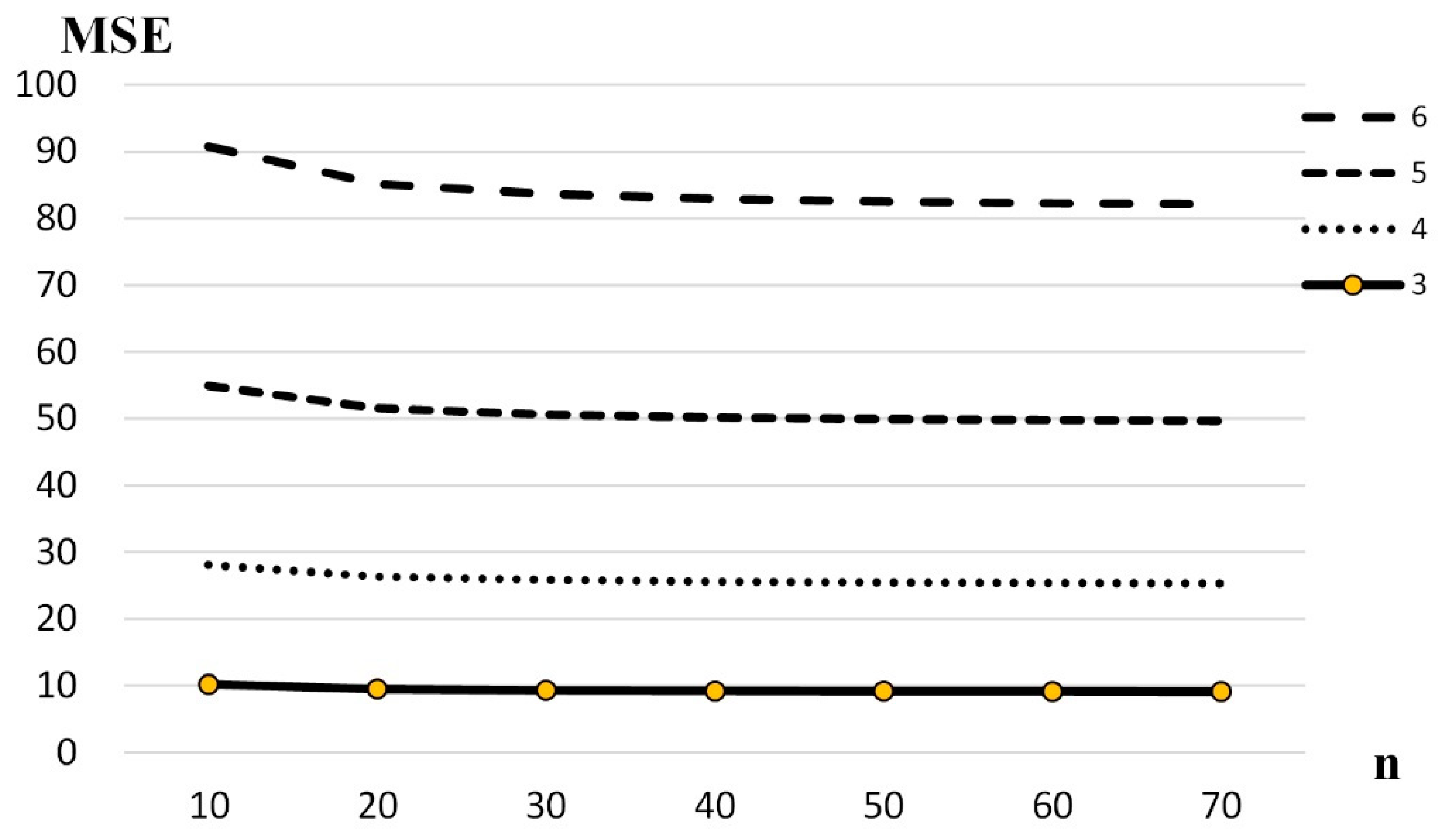
can be computed following Equations (12) and (15) under the assumption that the value of
k is 6, 5, 4, or 3 and the sample size (
n) is 10, 20, 30, 40, 50, 60, or 70. The results of these calculations are shown in
Table 1.
Figure 1 illustrates the relationship between
and sample size (
n) for
δ = 1/4. As the sample size increases,
tends to decrease to the same stable value for all
k.
Figure 2 presents the relationship between
and sample size for
δ = 1/4. As the sample size increases,
tends to decrease to the same stable value for all
k.
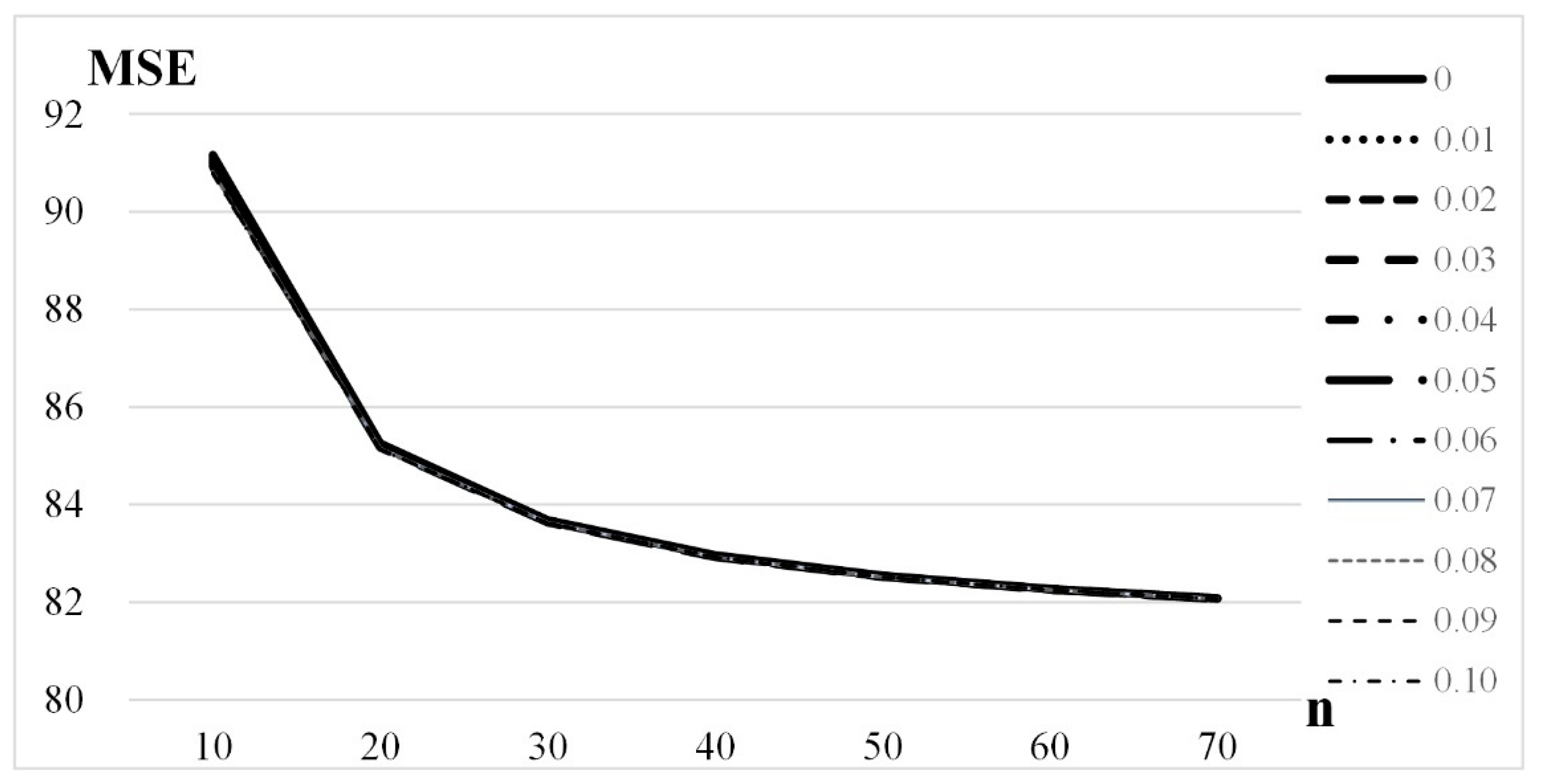
In addition, the influence of a small change in
δ on
and
is also worth discussing. Therefore, we calculate
with
δ increments of 0.01 according to Equations (12) and (15) for
k values of 6, 5, 4, or 3 and sample sizes of 10, 20, 30, 40, 50, 60, or 70. The results are shown in
Table 2.
Figure 3 illustrates the relationship between
and sample size for
k = 6. As the sample size increases,
tends to decrease to the same stable value for all
k.
Figure 4 shows the relationship between
and sample size for
k = 6. As the sample size increases,
tends to decrease to the same stable value for all
k.
3. Upper Confidence Limits of the Six Sigma Quality Index
As mentioned, under the assumption of normality,
follows the
distribution. Therefore,
T follows a
distribution. Thus, we have
To derive the
upper confidence limit on
, some events are defined as follows:
and
where
is the upper
quintile of
,
is the lower
quintile of
, and
is the confidence level. In fact,
and
. Based on Boole’s inequality and Morgan’s theorem,
This is equivalent to
where
Therefore, the
confidence interval of
can be calculated as follows:
is a function of parameter
and
. According to Chen et al. [
21], mathematical programming can be used to compute the upper confidence limit of
.
In this computation method,
is treated as the objective function, and the confidence region is regarded as the feasible solution area. Therefore, parameters
and
are the two decision variables of this objective function. The optimization problem can then be defined as follows:
The feasible solution area in this problem is a rectangle (convex set), and when
is closer to 0,
increases because
becomes closer to 1. Similarly, the value of
increases as the value of
γ decreases. Therefore,
increases as
approaches the origin. The maximum of
is obtained at the bottom of the rectangle. Therefore, the feasible solution area in this problem is a line segment (convex set). Thus, mathematical programming can be applied to determine the upper confidence limit of
. Consequently, the model for the index
can be rewritten as follows:
can be simplified to a function of
as follows:
Equation (25) shows that increases as becomes closer to 0.
Furthermore, the maximum value of is closely related to and . Hence, we consider three cases for and in this study.
- Case 1:
Because
, the maximum of
is obtained for
; this maximum is defined as
- Case 2:
Because
,
. Therefore, the maximum of
is obtained for
:
- Case 3:
Because
,
. Therefore, the maximum of
is obtained for
:
On the basis of the relationships described in Equations (26)–(28), we define
and
Subsequently, the
upper confidence limit of
can be obtained as follows:
4. Hypothesis Testing
As defined previously,
is a function of the process parameters
and
. To determine whether the process quality level reaches the
k sigma level, statistical hypothesis testing was conducted. The relationship between
and
should be constructed and then verified using a hypothesis test. A case study is presented to verify the proposed inferences in
Section 5.
Hypothesis testing entails the following steps:
- Step 1:
Determine the required process quality level.
The process quality level is assumed to be k sigma.
- Step 2:
Propose the null hypothesis and the alternative hypothesis .
The null and alternative hypotheses are as follows:
The upper confidence limit can then be obtained through statistical testing, and the hypotheses are judged as follows:
- (1)
If , then do not reject and conclude that
- (2)
If , then reject and conclude that
- Step 3:
Design the sampling plan.
The sample size and significance level α are assigned. Random sampling should then be conducted during the process control.
- Step 4:
Compute and to determine the suitable formula for .
The suitable formula for
can be determined on the basis of the three for
and
after these two parameters have been calculated from the original measurement data.
- Step 5:
Compare and k.
After has been computed, k and can be compared. The process capability is considered to reach Six Sigma level if .
5. A Case Study
This article proposed a new Six Sigma index, which can quickly and easily determine the process capability by simply calculating the value of the collected data. For managers and engineers, this index can be used to monitor the process in real time, taking into account the economy and immediacy.
To demonstrate the suitability of the proposed method for practical application, a case study from the semiconductor assembly process is presented as an example for statistical testing. A chip package with a leadframe carrier must pass through the plating process to provide protection for the metal plating layer and the medium, which are required for the subsequent surface-mounted technology (SMT) process. Because the plating thickness affects the SMT quality, process control is crucial at the plating stage. The plating layer on the outer lead of the leadframe is an important medium, providing a mechanical and electrical connection between the package and the printed circuit board (PCB). The composition and thickness of the plating layer affect the soldering quality between the package and the PCB. When the plating thickness exceeds the specification, the package body and the PCB cannot be effectively joined, resulting in an open-circuit or short-circuit current. In this study, the thickness specification for the plating layer was 550 ± 150 μm; that is, T = 550 μm and d = 150 μm.
The statistical testing procedure accords with the five steps defined in the previous section:
- Step 1:
Determine the required process quality level.
Six Sigma level (k = 6) is the desired process quality level for this case.
- Step 2:
Propose the null hypothesis and the alternative hypothesis .
The null and alternative hypotheses are as follows:
The upper confidence limit can be obtained through statistical testing, and the hypotheses are judged as follows:
- (1)
If , then do not reject and conclude that
- (2)
If , then reject and conclude that
- Step 3:
Design the sampling plan.
The sample size (n) and the significance level α are defined as 70 and 0.05, respectively.
- Step 4:
Compute and to determine the suitable formula for .
Because
and
are both less than 0.00,
I and
i are both 1.00, according to Equation (25). Finally,
- Step 5:
Compare and k.
Because , do not reject and conclude that . This result is consistent with the assumption that . That is, the minimum value of is 8.48, but it exceeds the required value of k (6) for a sample size of 70. Hence, statistical testing reveals that , and the process capability is considered to reach Six Sigma level.
6. Conclusions
A PCI is necessary for determining whether a process capability meets Six Sigma level, which is indicative of an extremely good process capability.
Following the research of Chen et al. [
21], this study employed
as a measure of process capability. However,
includes unknown parameters
and
. Therefore, statistical inference was used to verify
for different
k values and sample sizes (
n). Finally, the results revealed that
exhibit stable convergence trends. Furthermore, we derived the upper limit of
. First, Boole’s inequality and Morgan’s theorem were used to compute the error
, and linear programming was then applied to calculate the upper confidence limit
of
.
The maximum value of was separated into three categories based on the relationship between and .
The maximum value of was determined from a comparison of the combination of and with 0.00. Three combinations of and were explored in this study. For each combination, we obtained a general formula for .
Finally, a case study from the semiconductor assembly process was employed to verify the hypotheses of the Six Sigma quality index. For this case, was deduced to be 8.48 for k = 6 and n = 70. Therefore, was a valid hypothesis. That is, the process capability reached Six Sigma level.
This study utilized as a Six Sigma quality index to make statistical inferences, and the upper limits of the confidence intervals of point estimations were then obtained. The integrated definition of is simple and convenient for industrial application.
Author Contributions
Conceptualization, C.-C.T. and K.-S.C.; methodology, C.-C.T. and K.-S.C.; software, K.-C.C.; validation, K.-C.C.; formal analysis, C.-C.T. and K.-S.C.; investigation, C.-C.T. and K.-C.C.; resources, C.-C.T.; data curation, K.-C.C.; writing—original draft preparation, C.-C.T., K.-C.C. and K.-S.C.; writing—review and editing, C.-C.T. and K.-S.C.; visualization, C.-C.T.; supervision, K.-S.C.; project administration, C.-C.T.; funding acquisition, C.-C.T. All authors have read and agreed to the published version of the manuscript.
Funding
This work was supported by the Natural Science Foundation of Fujian, China under [grant number 2020R0164] and the Society Science Foundation of Fujian, China under [grant number FJ2020B025].
Data Availability Statement
Not applicable.
Conflicts of Interest
The authors declare no conflict of interest.
Appendix A
To obtain the mean square error of
, we first calculate the followings:
Therefore, the mean square error of may be obtained as:
References
- Montgomery, D.C. Introduction to Statistical Quality Control, 8th ed.; John Wiley & Sons, Inc.: New York, NY, USA, 2019. [Google Scholar]
- Yu, C.M.; Luo, W.J.; Hsu, T.H.; Lai, K.K. Two-Tailed Fuzzy Hypothesis Testing for Unilateral Specification Process Quality Index. Mathematics 2020, 8, 2129. [Google Scholar] [CrossRef]
- Wang, S.; Chiang, J.Y.; Tsai, T.R.; Qin, Y. Robust process capability indices and statistical inference based on model selection. Comput. Ind. Eng. 2021, 156, 107265. [Google Scholar] [CrossRef]
- Borgoni, R.; Zappa, D. Model-based process capability indices: The dry-etching semiconductor case study. Qual. Reliab. Eng. Int. 2020, 36, 2309–2321. [Google Scholar] [CrossRef]
- Juran, J.M. Juran’s Quality Control Handbook, 5th ed.; McGraw-Hill: New York, NY, USA, 1998. [Google Scholar]
- Kane, V.E. Process capability indices. J. Qual. Technol. 1986, 18, 41–52. [Google Scholar] [CrossRef]
- Boyles, R.A. The Taguchi capability index. J. Qual. Technol. 1991, 23, 17–26. [Google Scholar] [CrossRef]
- Tariq Aldowaisana, T.; Nourelfathb, M.; Hassan, J. Six Sigma performance for non-normal processes. Eur. J. Oper. Res. 2015, 247, 968–977. [Google Scholar] [CrossRef]
- Tjahjono, B.; Ball, P.; Vitanov, V.I.; Scorzafave, C.; Nogueira, J.; Calleja, J.; Minguet, M.; Narasimha, L.; Rivas, A.; Srivastava, A.; et al. Six sigma: A literature review. Int. J. Lean Six Sigma 2010, 1, 216–233. [Google Scholar] [CrossRef]
- Anand, R.B.; Shukla, S.K.; Ghorpade, A.; Tiwari, M.K.; Shankar, R. Six Sigma-based approach to optimise deep drawing operation variables. Int. J. Prod. Res. 2007, 45, 2365–2385. [Google Scholar]
- Coleman, S. Six Sigma: An opportunity for statistics and for statisticians. Significance 2008, 5, 94–96. [Google Scholar] [CrossRef]
- Hsu, C.; Chen, T.; Lii, P.; Hsu, S. Applying 6 sigma in quality improvement of TFT-LCD panel. J. Comput. Inf. Syst. 2011, 7, 1013–1020. [Google Scholar]
- Almazah, M.M.A.; Ali, F.A.M.; Eltayeb, M.M.; Atta, A. Comparative analysis four different ways of calculating yield index SSSpkBased on information of control chart, and six sigma, to measuring the process performance in industries: Case study in aden’s oil refinery, yemen. IEEE Access 2021, 9, 134005–134021. [Google Scholar] [CrossRef]
- Wang, C.C.; Chen, K.S.; Wang, C.H.; Chang, P.H. Application of 6-sigma design system to developing an improvement model for multi-process multi-characteristic product quality. Proc. Inst. Mech. Eng. Part B—J. Eng. Manuf. 2011, 225, 1205–1216. [Google Scholar] [CrossRef]
- Ouyang, L.Y.; Chen, K.S.; Yang, C.M.; Hsu, C.H. Using a QCAC–Entropy–TOPSIS approach to measure quality characteristics and rank improvement priorities for all substandard quality characteristics. Int. J. Prod. Res. 2014, 52, 3110–3124. [Google Scholar] [CrossRef]
- Wu, M.F.; Chen, H.Y.; Chang, T.C.; Wu, C.F. Quality evaluation of internal cylindrical grinding process with multiple quality characteristics for gear products. Int. J. Prod. Res. 2019, 57, 6687–6701. [Google Scholar] [CrossRef]
- Chen, K.S.; Chang, T.C. Construction and fuzzy hypothesis testing of Taguchi Six Sigma quality index. Int. J. Prod. Res. 2020, 58, 3110–3125. [Google Scholar] [CrossRef]
- Chen, K.S.; Wang, C.H.; Tan, K.H. Developing a fuzzy green supplier selection model using six sigma quality indices. Int. J. Prod. Econ. 2019, 212, 1–7. [Google Scholar] [CrossRef]
- Linderman, K.; Schroeder, R.G.; Zaheer, S.; Choo, A.S. Six Sigma: A goal-theoretic perspective. J. Oper. Manag. 2003, 21, 193–203. [Google Scholar] [CrossRef]
- Chen, K.S.; Ouyang, L.Y.; Hsu, C.H.; Wu, C.C. The Communion Bridge to Six Sigma and Process Capability Indices. Qual. Quant. 2009, 43, 463–469. [Google Scholar] [CrossRef]
- Chen, K.S.; Chen, H.T.; Chang, T.C. The construction and application of Six Sigma quality indices. Int. J. Prod. Res. 2017, 55, 2365–2384. [Google Scholar] [CrossRef]
- Pham, H. A New Criterion for Model Selection. Mathematics 2019, 7, 1215. [Google Scholar] [CrossRef] [Green Version]
| Publisher’s Note: MDPI stays neutral with regard to jurisdictional claims in published maps and institutional affiliations. |
© 2022 by the authors. Licensee MDPI, Basel, Switzerland. This article is an open access article distributed under the terms and conditions of the Creative Commons Attribution (CC BY) license (https://creativecommons.org/licenses/by/4.0/).


