On Some Examples of Trajectories in $\mathbb{R}$⁷

Abstract

In this paper we study the magnetic trajectories as the solutions of the Lorentz equation defined by the cross product corresponding to the 7-dimensional Euclidean space. We find several examples of such trajectories and moreover, we strongly motivate our results making a comparison with the 3-dimensional Euclidean case, ambient space which was among the first ones approached in the study of magnetic trajectories.

1. Introduction

As it is well known, the cross product gained the interest of scientists in many physical applications. For example, the cross product in the three dimensional Euclidean space is used to describe the angular velocity, the torque of a force, or even to describe the Lorentz force, $\overrightarrow{F}=q\overrightarrow{v}\times \overrightarrow{B}$, i.e., a force acting on a particle with charge q which moves at velocity $\overrightarrow{v}$ in a magnetic field $\overrightarrow{B}$. As it is well known, the magnetic curves in ${\mathbb{R}}^3$ are classified and the study was extended also for higher dimensional ambient spaces as follows.

Let $(M,g)$ be a complete Riemannian manifold endowed with the metric g. A closed 2-form on M defines a magnetic field F and its corresponding Lorentz force $\varphi$ is a $(1,1)$-tensor field $F(X,Y)=g(\varphi X,Y)$, $X,Y\in \mathfrak{X}\left(M\right)$. A smooth curve $\gamma$ on M is called a magnetic curve, or a trajectory corresponding to the the magnetic field F if it is a solution of the Lorentz equation ${\nabla }_{\dot{\gamma }}\dot{\gamma }=\varphi \dot{\gamma }$, where ∇ denotes the Levi-Civita connection associated to g on M. We easily notice that if the magnetic field vanishes, $F=0$, then the particle moves only under the influence of gravity, and hence the trajectory is a geodesic of M. Moreover, it was shown that the trajectories have constant speed. In our study we consider only arclength paramatrized trajectories, which are called normal trajectories.

The first results were obtained for the Landau-Hall problem— i.e., the study of the trajectories of charged particles moving on a surface under the influence of an uniform magnetic field. Recall that in the 2-dimensional case [1], the uniform magnetic fields (those magnetic fields which are parallel) are defined by the scalar multiples of the area element, $F=qd\mathcal{A}$, where q denotes the strength of the magnetic field. It was proven that the trajectories have constant curvature $\kappa =q$ on the surface. For example, on the plane ${\mathbb{R}}^2$ they are circles, on the 2-sphere ${\mathbb{S}}^2$ they are small circles and on the hyperbolic plane ${\mathbb{H}}^2(-1)$ the trajectories are either closed when $\left|q\right|\ge 1$, or open in rest. These results were extended to the study of trajectories on proper Kähler manifolds of any dimension (when the magnetic fields are defined as scalar multiples of the Kähler form) and it was proven [2] that they are circles, i.e., Frenet curves of osculating order 2 with (positive) constant geodesic curvature.

Next, in the 3-dimensional case $(M^3,g)$, the magnetic fields F are defined by the divergence free vector fields and it was shown that the magnetic background $(M^3,g,F)$ may be regarded as an almost contact metric manifold with closed fundamental 2-form. This problem was also generalized to arbitrary dimensions, in the study of trajectories corresponding to magnetic fields generated by closed fundamental 2-forms in Sasakian and cosympletic manifolds. In this situation it was proven that they are helices of osculating order 3.

Finally, since the Sasakian and cosymplectic manifolds are special classes of quasi-Sasakian manifolds, it was proven [3] that the magnetic curves in the quasi-Sasakian manifold ${\mathbb{R}}^{2(n+p)+1}$ are helices of osculating order 5. See also [4] for this result in ${\mathbb{R}}^5$. Another example is the study of trajectories in the generalized Heisenberg group $H(n,1)$ endowed with its quasi-Sasakian structure in [5], when it was proven that the trajectories are again helices of maximum order 5.

Going back now to the 3-dimensional case, a question that arises, is what changes in the study of trajectories in ${\mathbb{R}}^7$ using a higher-dimensional analogue of the cross product of two vectors from ${\mathbb{R}}^3$.

In the present paper we start from the definition of such a cross product in ${\mathbb{R}}^7$ introduced by Lounesto in [6] and we study the corresponding trajectories. The Section 2 consists of a collection of the necessary notions used in the following and the Section 3 describes in parallel the 3-dimensional and the 7-dimensional case. The Section 4 contains the main results we obtained. The Theorems 1 and 2 deal with the classification of trajectories in a hyperplane $H\subset {\mathbb{R}}^7$ and the unit 6-sphere ${\mathbb{S}}^6\subset {\mathbb{R}}^7$ respectively, meanwhile the Theorem 3 consists of some examples of trajectories on the cylinder ${\mathbb{S}}^5\times \mathbb{R}\subset {\mathbb{R}}^7$. Finally, we conclude with references.

2. Preliminaries

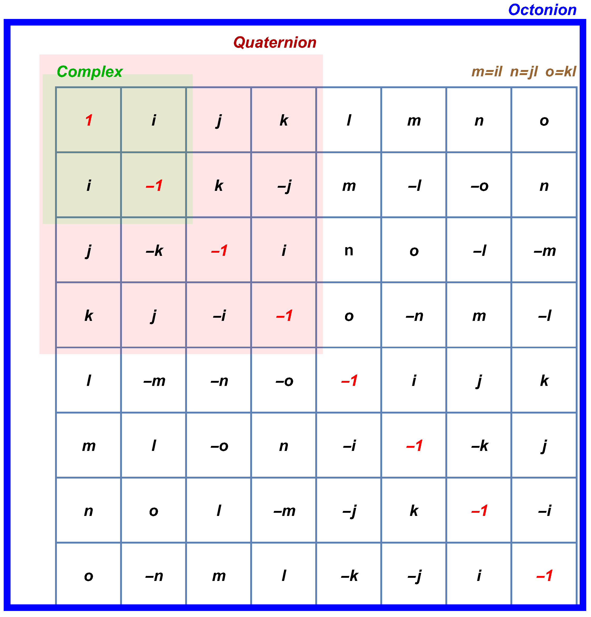
It is well known, see e.g., [6], that if we want to define a cross product with two factors in ${\mathbb{R}}^n$, and we ask for it to be orthogonal to both of the terms and to have the length equal to the area of the parallelogram constructed on the two vectors, then $n\in \{3,7\}$. See also [7]. Let us consider ${\mathbb{R}}^7$ endowed with the usual scalar product $⟨,⟩$. According to [6], the cross product of two vectors on $({\mathbb{R}}^7,⟨⟩$ can be defined using an orthonormal basis $\{e_1,\cdots ,e_7\}$ by antisymmetry $e_i\times e_j=-e_j\times e_i$ and $e_i\times e_{i+1}=e_{i+3}$, where the indices $i,j=\overline{1,7}$ are cyclically permuted and translated $mod7$. The table of operations is as follows:

Regarding the properties of the cross product,

• the orthogonality on the two factors: $⟨u\times v,u⟩=0,⟨u\times v,v⟩=0,$
• the Pythagorean theorem: ${\parallel u\times v\parallel }^2={\parallel u\parallel }^2{\parallel v\parallel }^2-{⟨u,v⟩}^2,$
  are both satisfied, while
• the Jacobi identity:

  $$J(u,v,w):=(u\times v)\times w+(v\times w)\times u+(w\times u)\times v=0,$$

unlike in the 3-dimensional case, it is not satisfied $\forall u,v,w\in {\mathbb{R}}^7$.

For this reason, the cross product does not give ${\mathbb{R}}^7$ the structure of a Lie algebra.

However, the vector triple product satisfies the following property:

$$u\times (v\times w)=⟨u,w⟩v-⟨u,v⟩w+\frac{1}{3}J(u,v,w).$$

Obviously, the vector triple formula from ${\mathbb{R}}^3$ is valid also in ${\mathbb{R}}^7$ if and only if $J(u,v,w)=0$, i.e., the Jacobi identity is also satisfied.

Moreover, we point out that the cross product in ${\mathbb{R}}^7$ does satisfy a generalization of the Jacobi identity, called the Malcev identity,

$$\begin{array}{cc}m(u,v,w):=\hfill & (u\times v)\times (u\times w)+u\times \left[\right(u\times v)\times w]-u\times [u\times (v\times w\left)\right]\hfill \\ & +v\times [u\times (u\times w)]=0,\forall u,v,w\in {\mathbb{R}}^7,\hfill \end{array}$$

which gives to ${\mathbb{R}}^7$ the structure of a Malcev algebra, see e.g., [8].

In fact, the multiplication rule given in Table 1 can be explained, briefly, in the following way. In analogy with $\mathbb{C}=\mathbb{R}\oplus \mathbb{R}i$ (the set of complex numbers) and $\mathbb{H}=\mathbb{C}\oplus \mathbb{C}j$ (the set of quaternions), it is still possible to define the set of octonions as $\mathbb{O}=\mathbb{H}\oplus \mathbb{H}l$, where l is an “imaginary unit” that does not belong to $\mathbb{H}$. See e.g., [9] or [8]. The multiplication rule is given in the Figure 1 (see also [10]).

Table 1. Multiplication rule for the cross product in ${\mathbb{R}}^7$.

×	${\mathit{e}}_1$	${\mathit{e}}_2$	${\mathit{e}}_3$	${\mathit{e}}_4$	${\mathit{e}}_5$	${\mathit{e}}_6$	${\mathit{e}}_7$
$e_1$	0	$e_4$	$e_7$	$-e_2$	$e_6$	$-e_5$	$-e_3$
$e_2$	$-e_4$	0	$e_5$	$e_1$	$-e_3$	$e_7$	$-e_6$
$e_3$	$-e_7$	$-e_5$	0	$e_6$	$e_2$	$-e_4$	$e_1$
$e_4$	$e_2$	$-e_1$	$-e_6$	0	$e_7$	$e_3$	$-e_5$
$e_5$	$-e_6$	$e_3$	$-e_2$	$-e_7$	0	$e_1$	$e_4$
$e_6$	$e_5$	$-e_7$	$e_4$	$-e_3$	$-e_1$	0	$e_2$
$e_7$	$e_3$	$e_6$	$-e_1$	$e_5$	$-e_4$	$-e_2$	0

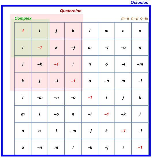
Figure 1. The multiplication rule in the set of octonions.

As a vector space, $\mathbb{O}$ can be decomposed as $\mathbb{O}=\mathbb{R}\oplus {\mathbb{R}}^7$, emphasizing the real part, and, respectively, the imaginary part of an octonion. Hence, ${\mathbb{R}}^7\equiv \mathrm{Im}\mathbb{O}$. If $u,v\in {\mathbb{R}}^7$ are purely imaginary octonions, then one can define a multiplication in ${\mathbb{R}}^7$ by

$$u\times v=\mathrm{Im}(u·v).$$

Hence, the octonion multiplication may be rewritten in an analogue way as in the case of quaternions, as

$$(a,u)·(b,v)=\left(ab-⟨u,v⟩,av+bu+u\times v\right),$$

where $(a,u),(b,v)\in \mathbb{O}=\mathbb{R}\oplus {\mathbb{R}}^7$.

Now, we take an orthonormal basis $\{e_1,e_2,\cdots ,e_7\}$ in ${\mathbb{R}}^7$, and we make the identification with $\{\mathit{i},\mathit{j},\mathit{k},\mathit{l},\mathit{m},\mathit{n},\mathit{o}\}$ from the Figure 1.

There are 480 possibilities of doing it. Let us make the following setting:

$$e_1=\mathit{i},e_2=\mathit{j},e_3=\mathit{o},e_4=\mathit{k},e_5=-\mathit{m},e_6=\mathit{l},e_7=\mathit{n}.$$

This leads us to the multiplication rule given in the Table 1. For more details on octonions, see e.g., [9,11,12] and references therein.

3. Trajectories in ${\mathbb{R}}^{\mathbf{3}}$ vs. ${\mathbb{R}}^{\mathbf{7}}$

In this section we emphasize the major differences between the study of magnetic curves in the 3-dimensional real space endowed with the usual cross product and the analogous study in the case of the 7-dimensional real space endowed with the cross product defined in the previous section.

As it was mentioned many times in some previous works on magnetic curves, the 3-dimensional case is very special.

In a generic 3-dimensional Riemannian manifold $(M^3,g)$ the 2-forms and the vector fields may be identified via the Hodge star operator ⋆ and the volume form $d{v}_g$ of $M^3$. Hence, the magnetic fields (corresponding to closed 2-forms) mean divergence free vector fields. Recall that some important examples of divergence free vector fields are the Killing vector fields and they define the so-called Killing magnetic fields. Classically, one can define the cross product on $M^3$ as $g(X\times Y,Z)=d{v}_g(X,Y,Z)$, $\forall X,Y\in \mathfrak{X}\left(M^3\right)$. If we denote by V a Killing vector field on $M^3$, then $F_V=d{v}_g(V,·,·)$ represents the corresponding Killing magnetic field.

Let $(x,y,z)$ be the global coordinates on ${\mathbb{E}}^3=({\mathbb{R}}^3,⟨,⟩)$. A basis of Killing vector fields is given by three translational vector fields and three rotational vector fields with respect to the coordinate axes ${\displaystyle \left\{\frac{\partial }{\partial z},\frac{\partial }{\partial y},\frac{\partial }{\partial x},x\frac{\partial }{\partial y}-y\frac{\partial }{\partial x},y\frac{\partial }{\partial z}-z\frac{\partial }{\partial y},z\frac{\partial }{\partial x}-x\frac{\partial }{\partial z}\right\}.}$

Let $\gamma :I\to {\mathbb{E}}^3$ be a normal magnetic curve, namely a solution of the magnetic equation (the Lorentz equation):

$$\ddot{\gamma }\left(s\right)=V\left(s\right)\times \dot{\gamma }\left(s\right),\mathrm{where}V\left(s\right)=V\left(\gamma \left(s\right)\right).$$

(1)

The Lorentz force has the expression:

$$\varphi :\mathfrak{X}\left({\mathbb{E}}^3\right)\to \mathfrak{X}\left({\mathbb{E}}^3\right),\varphi X=V\times X,\forall X\in \mathfrak{X}\left({\mathbb{E}}^3\right).$$

(2)

In order to solve the Lorentz Equation (1), the easiest case is to consider the constant Killing vector field $V_0=q{\displaystyle \frac{\partial }{\partial z}}$ (the other two translational Killing vector fields being treated similarly). The corresponding trajectories, up to the choice of the initial condition $\gamma \left(0\right)$, are parametrized by

$$\gamma \left(t\right)=\left({\displaystyle \frac{sin\theta }{q}}sin\left(qt\right),{\displaystyle \frac{sin\theta }{q}}cos\left(qt\right),tcos\theta \right),$$

and they represent helices with the axis given by $V_0$. More details can be found, for example, in [13,14].

Remark 1.

A more difficult situation occurs in the study of magnetic curves determined by the rotational Killing vector field $V=x{\displaystyle \frac{\partial }{\partial y}}-y{\displaystyle \frac{\partial }{\partial x}}$. The complete classification of these magnetic curves was done in [14] (see also [15]) and it consists in: planar curves situated in a vertical strip, circular helices and a class of curves for which the explicit parametrizations were provided, involving elliptic integrals.

At this point, let us consider V a constant vector field in ${\mathbb{R}}^7$ and we denote the Lorentz force $\varphi :\mathfrak{X}\left({\mathbb{R}}^7\right)\to \mathfrak{X}\left({\mathbb{R}}^7\right)$, $\varphi \left(X\right)=V\times X$ and the 2-form F on ${\mathbb{R}}^7$ given by $F(X,Y)=⟨\varphi X,Y⟩$. Now, we make the following observations:

• ${\varphi }^{2}X=V\times (V\times X)=⟨V,X⟩V-{\parallel V\parallel }^{2}X={\parallel V\parallel }^2\left(⟨{\displaystyle \frac{V}{\parallel V\parallel }},X⟩{\displaystyle \frac{V}{\parallel V\parallel }}-X\right),$
• The 2-form F is closed, that is $dF=0$, and hence it defines an magnetic field on ${\mathbb{R}}^7$.

The equation that leads us to the magnetic trajectories is:

$${\gamma }^{″}=V\times {\gamma }^{\prime },$$

(3)

where $\gamma :I\to {\mathbb{R}}^7$ is arclength parametrized.

In order to solve the Lorentz Equation (3), we decompose ${\gamma }^{\prime }$ as:

$${\gamma }^{\prime }=\alpha \left(t\right)V+W\left(t\right),$$

where $\alpha \in C^{\infty }\left(I\right)$, $W\left(t\right)\in {\mathbb{R}}^7$ and $W\left(t\right)\perp V$, $\forall t\in I$.

Since $\parallel {\gamma }^{\prime }\parallel =1$, it yields ${\parallel V\parallel }^2\alpha {\left(t\right)}^2+{\parallel W\left(t\right)\parallel }^2=1$, $\forall t\in \mathbb{R}$.

The Lorentz Equation (3) becomes:

$${\alpha }^{\prime }\left(t\right)V+W^{\prime }\left(t\right)=V\times W\left(t\right).$$

(4)

Taking the scalar product with V and taking into account $⟨W\left(t\right),V⟩=0$, $\forall t\in I$, we find

$${\alpha }^{\prime }\left(t\right){\parallel V\parallel }^2=0,\forall t\in I,$$

meaning that $\alpha$ is a constant function. Subsequently, (1) writes as:

$$W^{\prime }\left(t\right)=V\times W\left(t\right).$$

(5)

Taking the derivative with respect to t, we successively get:

$$W^{″}\left(t\right)=V\times W^{\prime }\left(t\right)=V\times \left(V\times W\left(t\right)\right)=⟨V,W\left(t\right)⟩V-{\parallel V\parallel }^{2}W\left(t\right)=-{\parallel V\parallel }^{2}W\left(t\right).$$

It follows that

$$W\left(t\right)=cos\left(qt\right)v_1+sin\left(qt\right)v_2,$$

where $q=\parallel V\parallel$, and $v_1$, $v_2$ are constant vectors in ${\mathbb{R}}^7$. Because ${\parallel W\left(t\right)\parallel }^2=1-{\alpha }^2{\parallel V\parallel }^2$, $\forall t\in I$, we must have $\parallel v_1\parallel =\parallel v_2\parallel =\sqrt{1-{\alpha }^2{\parallel V\parallel }^2}$ and $⟨v_1,v_2⟩=0$.

• Let ${\alpha }^2\ne 1/{\parallel V\parallel }^2$.

The Equation (5) implies, moreover, the conditions

$⟨v_1\times v_2,V⟩={\parallel V\parallel }^2\left(1-{\alpha }^2{\parallel V\parallel }^2\right)$ and $v_2={\displaystyle \frac{V}{\parallel V\parallel }}\times v_1$.

Hence,

$${\gamma }^{\prime }\left(t\right)=\left(cos\left(qt\right)v_1+sin\left(qt\right)v_2\right)+\alpha V.$$

We see that $\gamma$ is a helix in the 3-space defined by $\{v_1,v_2,V\}$ and having axis V.

• If $\alpha =0$, the curve $\gamma$ degenerates to a circle of radius ${\displaystyle \frac{1}{\parallel V\parallel }}$ in the 2-plane $\{v_1,v_2\}$.
• If $\alpha =\pm 1/\parallel V\parallel$, then $W\left(t\right)=0$, hence $\gamma$ is an integral curve for $\pm V$, namely it is a line.

Let us consider the following example:

Example 1.

Let $V=q{e}_1$, $q\ne 0$. The normal magnetic curves $\gamma :I\to {\mathbb{R}}^7$ corresponding to V with the property that $\gamma \left(0\right)=p_0$ and ${\gamma }^{\prime }\left(0\right)=cos\theta e_1+sin\theta e_2$, $\theta \in (0,\pi )$ are given by:

$$\gamma \left(t\right)=p_0+tcos\theta e_1+{\displaystyle \frac{1}{q}}sin\theta sin\left(qt\right)e_2+{\displaystyle \frac{1}{q}}sin\theta \left(1-cos\left(qt\right)\right)e_4.$$

We conclude this section with some final remarks on the structure of ${\mathbb{R}}^7$, where we define:

(i)

a vector field $\xi ={\displaystyle \frac{V}{\parallel V\parallel }}$;

(ii)

a 1-form $\eta$ such that $\eta \left(X\right)={\displaystyle \frac{⟨V,X⟩}{\parallel V\parallel }}$;

(iii)

$\phi :\mathfrak{X}\left({\mathbb{R}}^7\right)\to \mathfrak{X}\left({\mathbb{R}}^7\right)$, $\phi X=\xi \times X$.

The following relations are satisfied:

$$\eta \left(\xi \right)=1,\eta \circ \phi =0,{\phi }^2=-I+\eta \otimes \xi ,\phi \xi =0,$$

together with the compatibility condition:

$$⟨\phi X,\phi Y⟩=⟨\xi \times X,\xi \times Y⟩=-⟨X,\xi \times (\xi \times Y)⟩=-⟨X,⟨\xi ,Y⟩\xi -Y⟩=⟨X,Y⟩-⟨X,\xi ⟩⟨Y,\xi ⟩.$$

Thus, we have an almost contact metric structure. Even more, $\phi$ is parallel, thus the structure is cosymplectic.

For this reason, having in mind [16], the above result is not surprising. In the same spirit, also the fact that $\alpha$ is a constant function is a consequence of [16].

4. Main Results

Let us consider $M^6$ an oriented hypersurface in ${\mathbb{R}}^7$ having the unit normal N.

We define $J:\mathfrak{X}\left(M\right)\to \mathfrak{X}\left(M\right)$ by

$$X\mapsto JX=N\times X.$$

(6)

Recall that $N\times X\perp X$ from the properties of the cross product, hence $JX$ is tangent to M for any X tangent to M. Moreover, we have $J^{2}X=N\times (N\times X)=-X$, meaning that J defines an almost complex structure on M. Finally, J is compatible with the metric on M induced from the scalar product $⟨,⟩$ of ${\mathbb{R}}^7$.

$$⟨JX,JY⟩=⟨N\times X,N\times Y⟩=⟨X,Y⟩-⟨X,N⟩⟨Y,N⟩=⟨X,Y⟩,$$

for any X, Y tangent to M. This shows that $(M,J,⟨,⟩)$ inherits an almost Hermitian structure.

Let us denote by A the shape operator corresponding to N.

Proposition 1.

The covariant derivative of J can be expressed as

$$\left({\nabla }_{X}J\right)Y=-AX\times Y-⟨AX,JY⟩N,$$

for any X, Y tangent to M.

Proof. 

Let $\stackrel{\mathrm{o}}{\nabla }$ be the flat connection of ${\mathbb{R}}^7$. We have the Gauss and Weingarten formulas

$$\begin{array}{c}{\stackrel{\mathrm{o}}{\nabla }}_{X}Y={\nabla }_{X}Y+h(X,Y)N,\hfill \\ {\stackrel{\mathrm{o}}{\nabla }}_{X}N=-AX,\hfill \end{array}$$

where $h(X,Y)$ is the scalar second fundamental form of M in ${\mathbb{R}}^7$. The shape operator A and h are related by: $h(X,Y)=⟨AX,Y⟩$. We successively have

$$\begin{array}{cc}\left({\nabla }_{X}J\right)Y\hfill & ={\nabla }_X\left(JY\right)-J{\nabla }_{X}Y={\stackrel{\mathrm{o}}{\nabla }}_X\left(JY\right)-h(X,JY)N-J{\nabla }_{X}Y\hfill \\ \hfill & ={\stackrel{\mathrm{o}}{\nabla }}_X(N\times Y)-h(X,JY)N-N\times {\nabla }_{X}Y\hfill \\ \hfill & =-AX\times Y+N\times {\stackrel{\mathrm{o}}{\nabla }}_{X}Y-h(X,JY)N-N\times {\nabla }_{X}Y\hfill \\ \hfill & =-AX\times Y+N\times \left(h\right(X,Y\left)N\right)-h(X,JY)N\hfill \\ \hfill & =-AX\times Y-⟨AX,JY⟩N.\hfill \end{array}$$

□

We plan to study the trajectories corresponding to $\varphi =qJ$, namely to find those curves $\gamma :I\to M$ which satisfy the Lorentz equation:

$${\nabla }_{{\gamma }^{\prime }}{\gamma }^{\prime }=\varphi {\gamma }^{\prime },$$

(7)

where ∇ denotes the Levi-Civita connection on M and $q\in \mathbb{R}$ is the strength.

We consider the following three examples of hypersurfaces: a hyperplane, the unit sphere sphere ${\mathbb{S}}^6\left(1\right)$ and a cylinder ${\mathbb{S}}^5\times \mathbb{R}$.

4.1. Example 1. $M^6=H$

Thus, the hypersurface M is given by the hyperplane H endowed with the normal V (a unitary constant vector). It is well known that $M^6$ is totally geodesic in ${\mathbb{R}}^7$. From the Proposition 1 we get that the almost complex structure J is parallel, hence M is a Kähler manifold.

The normal magnetic trajectories are given by:

Theorem 1.

Let $M^6=H\subset ({\mathbb{R}}^7,⟨,⟩,\times )$ be a hypersurface endowed with the normal V—a unitary constant vector. Then, the normal magnetic curves in $H\subset {\mathbb{R}}^7$ are one of the following:

(i)

straight lines,

(ii)

circles parametrized as:

$$\gamma \left(t\right)=A_0+{\displaystyle \frac{1}{q}}\left(sin\left(qt\right)w-cos\left(qt\right)V\times w\right),$$

(8)

where w is a unitary constant vector, orthogonal to V.

Proof. 

The Lorentz Equation (7) becomes:

$${\gamma }^{″}=qV\times {\gamma }^{\prime }.$$

(9)

Remark that as $\gamma \left(t\right)\subset M$, $\forall t$, it follows that

$$⟨\gamma \left(t\right),V⟩=\mathrm{const}.⟺⟨{\gamma }^{\prime }\left(t\right),V⟩=0.$$

(10)

The solution is of the form

$${\gamma }^{\prime }\left(t\right)=cos\left(qt\right)w+sin\left(qt\right)V\times w,$$

(11)

where w is a (unitary) constant vector in ${\mathbb{R}}^7$, orthogonal to V. Obviously, if $q=0$, then we get the straight lines in the hyperplane M proving item $\left(i\right)$ from the theorem. If $q\ne 0$, then $\gamma$ is given by (8), which represents the parametrization of a circle, concluding the proof. □

4.2. Example 2. $M^6={\mathbb{S}}^6\left(1\right)$

For any $X,Y\in \mathfrak{X}\left({\mathbb{S}}^6\left(1\right)\right)$,

$${\nabla }_{X}Y={\stackrel{\mathrm{o}}{\nabla }}_{X}Y+⟨X,Y⟩p.$$

(12)

One considers ${\mathbb{S}}^6$ with its outward-pointing normal $N=p$; hence the shape operator is given by $AX=-X$. From the Proposition 1 we get

$$\left({\nabla }_{X}J\right)Y=X\times Y+⟨X,p\times Y⟩p,$$

for any X, Y tangent to ${\mathbb{S}}^6$.

Proposition 2

(See also [17]). The almost Hermitian structure defined on the unit 6-sphere is nearly Kähler.

Proof. 

One can easily show that $\left({\nabla }_{X}J\right)Y+\left({\nabla }_{Y}J\right)X=0,$ for any X, Y tangent to ${\mathbb{S}}^6$. □

Let us consider the trajectory $\gamma :I\to {\mathbb{S}}^6\left(1\right)$ parametrized by arclength. We have

$${\nabla }_{{\gamma }^{\prime }}{\gamma }^{\prime }={\gamma }^{″}+\gamma .$$

(13)

Consequently, the Lorentz Equation (7) becomes:

$${\gamma }^{″}+\gamma =q(\gamma \times {\gamma }^{\prime }).$$

(14)

The solutions of the Lorentz equation are described in the next result.

Theorem 2.

Let $M^6={\mathbb{S}}^6\left(1\right)\subset ({\mathbb{R}}^7,⟨,⟩,\times )$ be the unit 6-sphere. Then, the normal magnetic curves in ${\mathbb{S}}^6\left(1\right)\subset {\mathbb{R}}^7$ are circles which lie also on the sphere of center ${\displaystyle \frac{1}{\sqrt{q^2+1}}}{a}_0$ and radius ${\displaystyle \frac{1}{\sqrt{q^2+1}}}$ and they are parametrized as:

$$\gamma \left(t\right)={\displaystyle \frac{1}{\sqrt{q^2+1}}}\left(a_0+cos\left(\sqrt{q^2+1}t\right)w_1+sin\left(\sqrt{q^2+1}t\right)w_2\right),$$

(15)

where $a_0\in \mathrm{span}\{w_1,w_2\}$ and $w_1,w_2$ are two unitary and orthogonal vectors in ${\mathbb{R}}^7$. As usual, q denotes the strength.

Proof. 

First, let us notice that $\gamma \left(t\right)$ and ${\gamma }^{\prime }\left(t\right)$ are orthogonal. Second, regarding the curvatures of the trajectory, we get that the curvature of $\gamma$ in ${\mathbb{R}}^7$, ${\kappa }_0=\parallel {\gamma }^{″}\parallel$ is constant:

$${\kappa }_0^2=⟨{\gamma }^{″},{\gamma }^{″}⟩=⟨q(\gamma \times {\gamma }^{\prime })-\gamma ,q(\gamma \times {\gamma }^{\prime })-\gamma ⟩=q^2+1.$$

(16)

Thinking $\gamma$ as a curve in ${\mathbb{R}}^7$, we have

$$T={\gamma }^{\prime },{\nu }_1={\displaystyle \frac{1}{\sqrt{q^2+1}}}{\gamma }^{″},$$

(17)

where T denotes the tangent vector to $\gamma$ and ${\nu }_1$ is the first unitary normal vector. We compute now:

$${\nu }_1^{\prime }+{\kappa }_{0}T={\displaystyle \frac{1}{\sqrt{q^2+1}}}{\gamma }^{‴}+\sqrt{q^2+1}{\gamma }^{\prime }.$$

(18)

The relation (14) yields ${\gamma }^{‴}+{\gamma }^{\prime }=q(\gamma \times {\gamma }^{″})$ and using again this Formula (14), we get

$${\gamma }^{‴}+{\gamma }^{\prime }=q(\gamma \times (-\gamma +q(\gamma \times {\gamma }^{\prime })))=q^2\gamma \times (\gamma \times {\gamma }^{\prime })=-q^2{\gamma }^{\prime }.$$

(19)

From (18) we deduce that

$${\nu }_1^{\prime }+{\kappa }_{0}T=0,$$

(20)

namely $\gamma$ has the osculating order 2. As, its curvature is constant, it follows that $\gamma$ is a Riemannian circle.

From (20) and using the fact that $T={\gamma }^{\prime }$, it follows that there exists a constant vector $a_0\in {\mathbb{R}}^7$ such that

$${\nu }_1\left(t\right)+{\kappa }_0\gamma \left(t\right)=a_0,\forall t\in I.$$

(21)

Even more, this relation yields

$$∥\gamma \left(t\right)-{\displaystyle \frac{1}{{\kappa }_0}}{a}_0∥={\displaystyle \frac{1}{{\kappa }_0}}.$$

(22)

As a matter of fact, $\gamma$ lies also on the sphere of center ${\displaystyle \frac{1}{{\kappa }_0}}{a}_0$ and radius ${\displaystyle \frac{1}{{\kappa }_0}}$, where ${\kappa }_0=\sqrt{q^2+1}$. Moreover, from the same Equation (21) it follows that $a_0$ is orthogonal to ${\gamma }^{\prime }\left(t\right)$ $\forall t\in I$. The relation (21) writes as:

$${\gamma }^{″}\left(t\right)+(q^2+1)\gamma \left(t\right)=\sqrt{q^2+1}{a}_0,\forall t\in I.$$

We get the general solution for the trajectories:

$$\gamma \left(t\right)={\displaystyle \frac{1}{\sqrt{q^2+1}}}{a}_0+cos\left(\sqrt{q^2+1}t\right){\tilde{w}}_1+sin\left(\sqrt{q^2+1}t\right){\tilde{w}}_2,$$

(23)

where ${\tilde{w}}_1,{\tilde{w}}_2\in {\mathbb{R}}^7$.

From the condition $\parallel {\gamma }^{\prime }\left(t\right)\parallel =1$, $\forall t\in I$, we immediately deduce $\parallel {\tilde{w}}_1\parallel =\parallel {\tilde{w}}_2\parallel ={\displaystyle \frac{1}{\sqrt{q^2+1}}}$ and $⟨{\tilde{w}}_1,{\tilde{w}}_2⟩=0,$ see e.g., [18] for more details on this type of computations.

Denoting now $w_1=\sqrt{q^2+1}{\tilde{w}}_1$ and $w_2=\sqrt{q^2+1}{\tilde{w}}_2$ we obtain the parametrization (15) for $\gamma$:

$$\gamma \left(t\right)={\displaystyle \frac{1}{\sqrt{q^2+1}}}\left(a_0+cos\left(\sqrt{q^2+1}t\right)w_1+sin\left(\sqrt{q^2+1}t\right)w_2\right),$$

where $w_1$, $w_2$ are two unitary and orthogonal vectors in ${\mathbb{R}}^7$. Recalling now the fact that $\gamma$ lies on ${\mathbb{S}}^6\left(1\right)$, i.e., ${\parallel \gamma \left(t\right)\parallel }^2=1$, $\forall t\in I$, it follows that

$$\parallel a_0{\parallel }^2=q^2,⟨a_0,w_1⟩=0,⟨a_0,w_2⟩=0.$$

(24)

Thus, $a_0$ is situated in a space orthogonal to the 2-plane $\Pi =\mathrm{span}\{w_1,w_2\}$.

Hence, $\gamma$ is an Euclidean circle situated in the 2-plane $\Pi$, with the center in the point having the position vector ${\displaystyle \frac{1}{\sqrt{q^2+1}}}{a}_0$ and of radius ${\displaystyle \frac{1}{\sqrt{q^2+1}}}$. □

4.3. Example 3. $M^6={\mathbb{S}}^5\times \mathbb{R}$

In this case the hypersurface M is a cylinder in ${\mathbb{R}}^6\times \mathbb{R}$. Let us denote an orthonormal basis, such that ${\mathbb{R}}^6=\mathrm{span}\{e_1,\cdots ,e_6\}$ and $\mathbb{R}=\mathrm{span}\left\{e_7\right\}$. If $(p,z)\in {\mathbb{S}}^5\times \mathbb{R}$, then the unitary normal at $(p,z)$ to M is given by $N_{(p,z)}=(p,0)$.

Let us consider the trajectory $\gamma :I\to {\mathbb{S}}^5\times \mathbb{R}$ denoted by

$$\gamma \left(t\right)=\left(x\left(t\right),f\left(t\right)\right),$$

(25)

where $x:I\to {\mathbb{S}}^5$ and $f:I\to \mathbb{R}$ are differential functions. Thus, $\parallel x\left(t\right)\parallel =1$, $\forall t\in I$. The arclength parametrization condition for $\gamma$ writes as:

$$\parallel x^{\prime }{\left(t\right)\parallel }^2+f^{\prime }{\left(t\right)}^2=1,\forall t\in I.$$

We have

$${\gamma }^{″}={\nabla }_{{\gamma }^{\prime }}{\gamma }^{\prime }+⟨A{\gamma }^{\prime },{\gamma }^{\prime }⟩(x,0).$$

(26)

If $X=(X_1,\cdots ,X_7)$ is tangent to $M^6\subset {\mathbb{R}}^6\times \mathbb{R}$, then $AX=-X+X_7{e}_7$.

Since ${\nabla }_{{\gamma }^{\prime }}{\gamma }^{\prime }=qN\times {\gamma }^{\prime }$, the Equation (26) can be rewritten as:

$$x^{″}+f^{″}{e}_7=q(x\times x^{\prime }+f^{\prime }x\times e_7)-{\parallel x^{\prime }\parallel }^{2}x.$$

(27)

Obviously, since $x\times e_7$ is orthogonal to $e_7$, it belongs to ${\mathbb{R}}^6$. Moreover, $\parallel x\times e_7{\parallel }^2=1$. But $x\times x^{\prime }$ has components both in ${\mathbb{R}}^6$ and $\mathbb{R}=\mathrm{span}\left\{e_7\right\}$.

Dealing with all the seven components of $\gamma$ being non-vanishing is a really challenging task. For this reason, we plan to find some examples of trajectories on the cylinder ${\mathbb{S}}^5\times \mathbb{R}$, leaving open the problem of the complete classification of these trajectories.

Theorem 3.

Let $M^6={\mathbb{S}}^5\times \mathbb{R}\subset ({\mathbb{R}}^7,⟨,⟩,\times )$ be a cylinder in ${\mathbb{R}}^6\times \mathbb{R}$, and we consider an orthonormal basis such that ${\mathbb{R}}^6=\mathrm{span}\{e_1,e_2,\cdots ,e_6\}$ and $\mathbb{R}=\mathrm{span}\left\{e_7\right\}$. The next curves

$$\gamma :I\to {\mathbb{S}}^5\times \mathbb{R}\gamma \left(t\right)=(\underset{x\left(t\right)}{\underbrace{x_1\left(t\right),x_2\left(t\right),\cdots ,x_6\left(t\right)}},f\left(t\right)),$$

are examples of magnetic trajectories, as follows:

(i) 

For $x\left(t\right)=e_i$ with a certain $i=\overline{1,6}$, $\gamma \left(t\right)=e_i+t{e}_7$ is a straight line parallel to $e_7$, that is a geodesic.

(ii) 

For $q=0$, the trajectory γ is a helix on a cylinder ${\mathbb{S}}^1\times R\subset M^6$ parametrized by:

$$\gamma \left(t\right)=w_{1}cos\left(at\right)+w_{2}sin\left(at\right)+(\lambda t+\mu )e_7,$$

(28)

where $a,\lambda ,\mu \in \mathbb{R}$ such that $a^2+{\lambda }^2=1$ and $\{w_1,w_2\}$ is an orthonormal basis in a 2-dimensional vector space W in ${\mathbb{R}}^6$.

(iii) 

For $x\left(t\right)=x_1\left(t\right)e_1+x_j\left(t\right)e_j$, with a certain $j=\overline{2,6}$, we distinguish two cases:

$\begin{array}{|c|}\hline j=3\\ \hline\end{array}$ The trajectory γ is given by:

$$\gamma \left(t\right)=\left(cos\theta \left(t\right),0,sin\theta \left(t\right),0,0,0,f\left(t\right)\right),where$$

(29)

$$\begin{array}{c}\hfill \theta \left(t\right)=\lambda -{\displaystyle \frac{1}{q}}cos(qt+{\psi }_0),\lambda ,{\psi }_0\in \mathbb{R},\end{array}$$

(30)

$$\begin{array}{c}\hfill f\left(t\right)=\mu -{\displaystyle \frac{1}{q}}sin(qt+{\psi }_0),\mu \in \mathbb{R}.\end{array}$$

(31)

$\begin{array}{|c|}\hline j\ne 3\\ \hline\end{array}$ Depending on the function $\theta \left(t\right)$, we have:

*

If $\theta \left(t\right)$ is constant, then γ is a vertical line on the cylinder.

*

If $\theta \left(t\right)=\epsilon t+{\theta }_0$, where $\epsilon =\pm 1$ and ${\theta }_0\in \mathbb{R}$, then γ is a horizontal circle:

$$\gamma \left(t\right)=\left(cos(\epsilon t+{\theta }_0),0,\cdots ,sin(\epsilon t+{\theta }_0),\cdots ,0,z_0\right).$$

(32)

(iv) 

For $x\left(t\right)=x_1\left(t\right)e_1+x_2\left(t\right)e_2+x_i\left(t\right)e_i$, $2<i\le 6$, we study all the possible cases for i and when $i=4$ it follows that γ is an Euclidean circle on ${\mathbb{S}}^2\subset {\mathbb{S}}^5$.

(v) 

For $x\left(t\right)=x_1\left(t\right)e_1+x_2\left(t\right)e_2+x_3\left(t\right)e_3+x_6\left(t\right)e_6$, we define

$$\gamma \left(t\right)=\left(r_{1}cosU\left(t\right),r_{2}cosU\left(t\right),r_{1}sinU\left(t\right),0,0,r_{2}sinU\left(t\right),f\left(t\right)\right),$$

where

$$\begin{array}{c}\hfill U\left(t\right)={\mu }_{1}cos\left(qt\right)+{\mu }_{2}sin\left(qt\right)-{\displaystyle \frac{c_0}{q}},\end{array}$$

(33)

$$\begin{array}{c}\hfill f\left(t\right)={\mu }_{1}sin\left(qt\right)-{\mu }_{2}cos\left(qt\right),\end{array}$$

(34)

and ${\mu }_1,{\mu }_2,r_1,r_2\in \mathbb{R}$ such that $r_1^2+r_2^2=1$. Then γ is a magnetic curve on ${\mathbb{S}}^5\times \mathbb{R}$.

Proof. 

In the sequel, we study step by step the all above cases.

Case (i)

$x\left(t\right)=e_i$, for a certain $i=1,\cdots ,6$.

Hence, $\gamma \left(t\right)=(0,\cdots ,1,\cdots ,0,f(t\left)\right)$, i.e., ${\gamma }^{\prime }$ is parallel to $e_7$. From the arclength parametrization condition we have $f^{\prime }\left(t\right)=\pm 1$ and consequently ${\gamma }^{\prime }\left(t\right)=\pm e_7$. The Equation (27) is not satisfied in general, unless if (and only if) $q=0$. Anyway, we know that the straight lines parallel to $e_7$ and situated on $M^6$ are geodesics.

Case (ii)

$q=0$.

Replacing $q=0$ in the Equation (27), it yields: $x^{″}=-{\parallel x^{\prime }\parallel }^{2}x$ and $f^{″}=0$. Thus, $f^{\prime }=\lambda \in \mathbb{R}$, $\parallel x^{\prime }\parallel =a\in \mathbb{R}$ such that $a^2+{\lambda }^2=1$. Subsequently, $f\left(t\right)=\lambda t+\mu$, $\mu \in \mathbb{R}$, and $x\left(t\right)=w_{1}cos\left(at\right)+w_{2}sin\left(at\right)$, $a\in [0,1]$. From the fact that $\parallel x\parallel =1$, it follows that $\{w_1,w_2\}$ is an orthonormal basis in a 2-dimensional vector space W in ${\mathbb{R}}^6$. Hence, $x\left(t\right)$ is a unitary circle in W. In this manner, we proved that when the strength of the magnetic field vanishes, the trajectory is parametrized by (28).

Case (iii)

$x\left(t\right)=x_i\left(t\right)e_i+x_j\left(t\right)e_j$, for $1\le i<j\le 6$.

In this case $\gamma \left(t\right)=(0,\cdots ,x_i,\cdots ,x_j,\cdots ,0,f)$. The relation $x_i^2+x_j^2=1$ yields $x_i=cos\theta \left(t\right)$ and $x_j=sin\theta \left(t\right)$, where $\theta \in {\mathcal{C}}^{\infty }\left(I\right).$

The arclength condition leads to ${\theta }^{\prime }{\left(t\right)}^2+f^{\prime }{\left(t\right)}^2=1$.

Let us fix $i=1$, $j>1$, $j\ne 7$. The Equation (27) becomes:

$$\begin{array}{cc}\hfill x_1^{″}\left(t\right)e_1+x_j^{″}\left(t\right)e_j+f^{″}\left(t\right)e_7& =q\left(x_1\left(t\right)x_j^{\prime }\left(t\right)-x_j\left(t\right)x_1^{\prime }\left(t\right)\right)e_1\times e_j\hfill \\ \hfill & +q{f}^{\prime }\left(t\right)\left(-x_1\left(t\right)e_3+x_j\left(t\right)e_j\times e_7\right)\hfill \\ \hfill & -{\theta }^{\prime }{\left(t\right)}^2\left(x_1\left(t\right)e_1+x_j\left(t\right)e_j\right).\hfill \end{array}$$

(35)

Computing now the scalar product with $e_j$ we get:

$$x_j^{″}\left(t\right)=-q{x}_1\left(t\right)f^{\prime }\left(t\right)⟨e_3,e_j⟩-{\theta }^{\prime }{\left(t\right)}^2{x}_j\left(t\right).$$

(36)

Subsequently, we distinguish two situations for j, as $j=3$ and $j\ne 3$.

$\begin{array}{|c|}\hline j=3\\ \hline\end{array}$ The Equation (35) writes as:

$$\begin{array}{cc}\hfill x_1^{″}\left(t\right)e_1+x_3^{″}\left(t\right)e_3+f^{″}\left(t\right)e_7& =q\left(x_1\left(t\right)x_3^{\prime }\left(t\right)-x_3\left(t\right)x_1^{\prime }\left(t\right)\right)e_7+q{f}^{\prime }\left(t\right)\left(-x_1\left(t\right)e_3+x_3\left(t\right)e_1\right)\hfill \\ \hfill & -{\theta }^{\prime }{\left(t\right)}^2\left(x_1\left(t\right)e_1+x_3\left(t\right)e_3\right).\hfill \end{array}$$

Since the vectors $\{e_1,e_3,e_7\}$ are linearly independent, we have:

$$\left\{\begin{array}{c}{x}_1^{″}\left(t\right)=q{f}^{\prime }\left(t\right)x_3\left(t\right)-{\theta }^{\prime }{\left(t\right)}^2{x}_1\left(t\right),\hfill \\ x_3^{″}\left(t\right)=q{f}^{\prime }\left(t\right)x_1\left(t\right)-{\theta }^{\prime }{\left(t\right)}^2{x}_3\left(t\right),\hfill \\ f^{″}\left(t\right)=q\left(x_1\left(t\right)x_3^{\prime }\left(t\right)-x_3\left(t\right)x_1^{\prime }\left(t\right)\right).\hfill \end{array}\right.$$

(37)

We wish to express everything in terms of $\theta$.

Using $x_1\left(t\right)=cos\theta \left(t\right)$ and $x_3\left(t\right)=sin\theta \left(t\right)$, we obtain:

$$({\theta }^{″}\left(t\right)+q{f}^{\prime }\left(t\right))sin\theta \left(t\right)=0,({\theta }^{″}\left(t\right)+q{f}^{\prime }\left(t\right))cos\theta \left(t\right)=0,f^{″}\left(t\right)-q{\theta }^{\prime }\left(t\right)=0.$$

(38)

Let $q\ne 0$. The first two equations of (38) immediately yield ${\theta }^{″}\left(t\right)+q{f}^{\prime }\left(t\right)=0$ and combining it with the third equation of (38) we get:

$${\theta }^{\prime }\left(t\right)=c_{1}cos\left(qt\right)+c_{2}sin\left(qt\right),f^{\prime }\left(t\right)=c_{1}sin\left(qt\right)-c_{2}cos\left(qt\right),c_1,c_2\in \mathbb{R}.$$

But ${\theta }^{\prime }{\left(t\right)}^2+f^{\prime }{\left(t\right)}^2=1$, $\forall t\in I$, which implies $c_1^2+c_2^2=1$. Thus, let us consider $c_1=sin{\psi }_0$ and $c_2=cos{\psi }_0$, ${\psi }_0\in \mathbb{R}$. Now, the previous relation writes as

$${\theta }^{\prime }\left(t\right)=sin(qt+{\psi }_0),f^{\prime }\left(t\right)=-cos(qt+{\psi }_0).$$

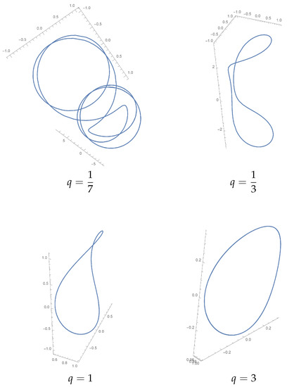
At this point, the expressions of $\theta$ and f are given by (30) and respectively (31), and the trajectory $\gamma$ is parametrized by (29). We plot some examples of such trajectories in the Figure 2, where $\lambda =\mu ={\psi }_0=0$ and the charge q is specified each time.

Figure 2. Trajectories in ${\mathbb{S}}^5\times \mathbb{R}$.

Remark 2.

Notice that when the strength $q\to 0$, the trajectory tends to a straight line, and when $q\to \infty$ the trajectory tends to a circle. Obviously, these two cases for γ are geodesics.

Remark 3.

If we look at the parametrization of the trajectory γ given by (28) in the case (ii) when $q=0$ and we ask for the 2-dimensional vector space W to be spanned by $e_1$ and $e_3$, it follows that

$$\gamma \left(t\right)=cos(at+b)e_1+sin(at+b)e_3+(\lambda t+\mu )e_7,$$

and it represents a circular helix in the space spanned by $\{e_1,e_3,e_7\}$.

$\begin{array}{|c|}\hline j\ne 3\\ \hline\end{array}$ The Equation (36) becomes $cos\theta \left(t\right){\theta }^{″}\left(t\right)=0.$

We assume that $\theta \left(t\right)$ is a non-constant function, otherwise the trajectory $\gamma$ is a vertical line on the cylinder $M^6$, hence a geodesic, which implies further that the strength vanishes, $q=0$. Summarizing, ${\theta }^{″}\left(t\right)=0$, namely $\theta \left(t\right)$ is an afine function.

Let us see what we obtain computing different scalar products in (35):

→

$⟨·,e_1⟩$ does not furnish new information, since $⟨e_j\times e_7,e_1⟩=0$ for $j\ne 3$.

→

$⟨·,e_3⟩$ yields $q{f}^{\prime }\left(t\right)x_1\left(t\right)=0$, since $⟨e_1\times e_j,e_3⟩=0$, $⟨e_j,e_3⟩=0$.

→

$⟨·,e_7⟩$ yields $f^{″}\left(t\right)=0$, since $⟨e_1\times e_j,e_7⟩=0$ for $j\ne 3$.

We conclude that $f\left(t\right)$ is a constant function, let us denote it $z_0$. Thus, the trajectory $\gamma$ is a horizontal circle, parametrized by (32).

Case (iv)

$x\left(t\right)=x_1\left(t\right)e_1+x_2\left(t\right)e_2+x_i\left(t\right)e_i$, for $2<i\le 6$.

Now $\gamma \left(t\right)=(x_1\left(t\right),x_2\left(t\right),0,\cdots ,x_i\left(t\right),\cdots ,0,f\left(t\right))$, as $x_1^2\left(t\right)+x_2^2\left(t\right)+x_i^2\left(t\right)=1$ and $x_1^{\prime }{\left(t\right)}^2+x_2^{\prime }{\left(t\right)}^2+x_i^{\prime }{\left(t\right)}^2+f^{\prime }{\left(t\right)}^2=1$. Back in Equation (27):

$$\begin{array}{cc}\hfill x_1^{″}\left(t\right)e_1+& x_2^{″}\left(t\right)e_2+x_i^{″}\left(t\right)e_i+f^{″}\left(t\right)e_7\hfill \\ \hfill & =q\left(x_1\left(t\right)e_1+x_2\left(t\right)e_2+x_i\left(t\right)e_i\right)\times \left(x_1^{\prime }\left(t\right)e_1+x_2^{\prime }\left(t\right)e_2+x_i^{\prime }\left(t\right)e_i\right)\hfill \\ \hfill & +q{f}^{\prime }\left(t\right)\left(x_1\left(t\right)e_1+x_2\left(t\right)e_2+x_i\left(t\right)e_i\right)\times e_7\hfill \\ \hfill & -\parallel x^{\prime }{\left(t\right)\parallel }^2\left(x_1\left(t\right)e_1+x_2\left(t\right)e_2+x_i\left(t\right)e_i\right).\hfill \end{array}$$

(39)

We compute

$$\begin{array}{c}x\times x^{\prime }=(x_1{x}_2^{\prime }-x_2{x}_1^{\prime })e_4+(x_1{x}_i^{\prime }-x_i{x}_1^{\prime })e_1\times e_i+(x_2{x}_i^{\prime }-x_i{x}_2^{\prime })e_2\times e_i,\hfill \\ x\times e_7=-x_1{e}_3-x_2{e}_6+x_i{e}_i\times e_7.\hfill \end{array}$$

(40)

We study in the sequel all the four possible values for i.

$\begin{array}{|c|}\hline i=3\\ \hline\end{array}$ The relations (40) become:

$$\begin{array}{c}x\times x^{\prime }=(x_1{x}_2^{\prime }-x_2{x}_1^{\prime })e_4+(x_1{x}_3^{\prime }-x_3{x}_1^{\prime })e_7+(x_2{x}_3^{\prime }-x_3{x}_2^{\prime })e_5,\hfill \\ x\times e_7=-x_1{e}_3-x_2{e}_6+x_3{e}_1.\hfill \end{array}$$

Replacing now in (39) and identifying the coefficients, we find

$e_1$: $x_1^{″}=q{f}^{\prime }{x}_3-{\parallel x^{\prime }\parallel }^2{x}_1$,	$e_5$: $0=q(x_2{x}_3^{\prime }-x_3{x}_2^{\prime })$,
$e_2$: $x_2^{″}=-{\parallel x^{\prime }\parallel }^2{x}_2$,	$e_6$: $0=-q{f}^{\prime }{x}_2$,
$e_3$: $x_3^{″}=-q{f}^{\prime }{x}_1-{\parallel x^{\prime }\parallel }^2{x}_3$,	$e_7$: $f^{″}=q(x_1{x}_3^{\prime }-x_3{x}_1^{\prime })$,
$e_4$: $0=q(x_1{x}_2^{\prime }-x_2{x}_1^{\prime })$.

From the relation given by the coefficient of $e_6$, it follows that $q{f}^{\prime }\left(t\right)=0$, and since $q\ne 0$ it follows that $f\left(t\right)=z_0$ is a constant function, thus the trajectory $\gamma$ is a curve on ${\mathbb{S}}^5$, but, basically, it lies on a sphere ${\mathbb{S}}^2\subset {\mathbb{S}}^5$. Some consequences:

$$\parallel x^{\prime }\parallel =1,x_1^{″}\left(t\right)+x_1=0,x_2^{″}\left(t\right)+x_2=0,x_3^{″}\left(t\right)+x_3=0,$$

which yield:

$$x_1\left(t\right)=a_{1}cost+a_{2}sint,x_2\left(t\right)=b_{1}cost+b_{2}sint,x_3\left(t\right)=c_{1}cost+c_{2}sint,$$

(41)

where $a_1,a_2,b_1,b_2,c_1,c_2\in \mathbb{R}$.

Moreover, for $q\ne 0$, we have also:

$$x_1{x}_2^{\prime }=x_2{x}_1^{\prime },x_2{x}_3^{\prime }=x_3{x}_2^{\prime },x_1{x}_3^{\prime }=x_3{x}_1^{\prime },$$

and using now (41) we obtain

$$\begin{array}{cc}{x}_1{x}_2^{\prime }\hfill & =(a_{1}cost+a_{2}sint)(b_{2}cost-b_{1}sint)\hfill \\ \hfill & =a_1{b}_2{cos}^{2}t-a_2{b}_1{sin}^{2}t+(a_2{b}_2-a_1{b}_1)sintcost,\hfill \\ x_2{x}_1^{\prime }\hfill & =a_2{b}_1{cos}^{2}t-a_1{b}_2{sin}^{2}t+(a_2{b}_2-a_1{b}_1)sintcost.\hfill \end{array}$$

Subtracting these two relations, we have $a_1{b}_2=a_2{b}_1$. Analogously, we obtain $b_2{c}_1=b_1{c}_2$ and $a_1{c}_2=a_2{c}_1$. If $a_2=0$, then $a_1\ne 0$, that implies $b_2=0$ and $c_2=0$. If $a_2\ne 0$, then $b_2\ne 0$ and $c_2\ne 0$. As ${\displaystyle \frac{a_1}{a_2}}={\displaystyle \frac{b_1}{b_2}}={\displaystyle \frac{c_1}{c_2}}$, it follows that there exists a real constant $\mu$ such that $a_2=\mu a_1$, $b_2=\mu a_2$, $c_2=\mu a_3$ and now, the expressions (41) become:

$$(x_1,x_2,x_3)=(cost+\mu sint)(a_1,b_1,c_1).$$

This relation is valid also for $a_2=0$, case when $\mu =0$.

Checking now the condition

$$1=\parallel x^{\prime }{\parallel }^2={(\mu cost-sint)}^2{\parallel (a_1,b_1,c_1)\parallel }^2,\forall t\in I,$$

it is false, thus $q=0$. This situation was described in the case (ii) of the proof.

$\begin{array}{|c|}\hline i=4\\ \hline\end{array}$ The relations (40) become:

$$\begin{array}{c}x\times x^{\prime }=(x_1{x}_2^{\prime }-x_2{x}_1^{\prime })e_4-(x_1{x}_4^{\prime }-x_4{x}_1^{\prime })e_2+(x_2{x}_4^{\prime }-x_4{x}_1^{\prime })e_1,\hfill \\ x\times e_7=-x_1{e}_3-x_2{e}_6-x_4{e}_5.\hfill \end{array}$$

Replacing now in (39) and identifying the coefficients, we have

$e_1$: $x_1^{″}=q(x_2{x}_4^{\prime }-x_4{x}_1^{\prime })-{\parallel x^{\prime }\parallel }^2{x}_1$,	$e_5$: $0=-q{f}^{\prime }{x}_4$,
$e_2$: $x_2^{″}=-q(x_1{x}_4^{\prime }-x_4{x}_1^{\prime })-{\parallel x^{\prime }\parallel }^2{x}_2$,	$e_6$: $0=-q{f}^{\prime }{x}_2$,
$e_3$: $0=-q{f}^{\prime }{x}_1$,	$e_7$: $f^{″}=0$,
$e_4$: $x_4^{″}=q(x_1{x}_2^{\prime }-x_2{x}_1^{\prime })-{\parallel x^{\prime }\parallel }^2{x}_4$.

We deduce that $q{f}^{\prime }\left(t\right)=0$, namely the trajectory $\gamma \left(t\right)\in {\mathbb{S}}^2\times \left\{z_0\right\}\subset {\mathbb{S}}^5\times \left\{z_0\right\}$. We set $q\ne 0$. In other words, $\gamma$ lies in ${\mathbb{S}}^2\times \mathbb{R}\subset {\mathbb{S}}^5\times \mathbb{R}$. Thus, $\parallel x^{\prime }{\parallel }^2=1$ and it yields:

$$x_1^{″}+x_1=q(x_2{x}_4^{\prime }-x_4{x}_1^{\prime }),x_2^{″}+x_2=q(x_4{x}_1^{\prime }-x_1{x}_4^{\prime }),x_4^{\prime \prime }+x_4=q(x_1{x}_2^{\prime }-x_2{x}_1^{\prime }).$$

(42)

If we consider $x=(x_1,x_2,x_4)\in {\mathbb{R}}^3$, then the above system of equations can be rewritten as $x^{″}+x=qx\times x^{\prime }$, where in this case × denotes the cross product in ${\mathbb{R}}^3$. The curve x in ${\mathbb{R}}^3$ has constant curvature $\sqrt{q^2+1}$ and we deduce that it is an Euclidean circle (we know that $x\subset {\mathbb{S}}^2\subset {\mathbb{R}}^3$).

$\begin{array}{|c|}\hline i=5\\ \hline\end{array}$ The relations (40) become:

$$\begin{array}{c}x\times x^{\prime }=(x_1{x}_2^{\prime }-x_2{x}_1^{\prime })e_4+(x_1{x}_5^{\prime }-x_5{x}_1^{\prime })e_6-(x_2{x}_5^{\prime }-x_5{x}_2^{\prime })e_3,\hfill \\ x\times e_7=-x_1{e}_3-x_2{e}_6+x_5{e}_4.\hfill \end{array}$$

Replacing now in (39) and identifying the coefficients,

$e_1$: $x_1^{″}=-{\parallel x^{\prime }\parallel }^2{x}_1$	$e_5$: $x_5^{″}=-{\parallel x^{\prime }\parallel }^2{x}_5$
$e_2$: $x_2^{″}=-{\parallel x^{\prime }\parallel }^2{x}_2$	$e_6$: $0=q(x_1{x}_5^{\prime }-x_5{x}_1^{\prime })-q{f}^{\prime }{x}_2$
$e_3$: $0=-q(x_2{x}_5^{\prime }-x_5{x}_2^{\prime })-q{f}^{\prime }{x}_1$	$e_7$: $f^{″}=0$.
$e_4$: $0=q(x_1{x}_2^{\prime }-x_2{x}_1^{\prime })+q{f}^{\prime }{x}_5$

We immediately notice that $f^{\prime }$ is constant, let us denote it by $\sigma \in [0,1]$ and it yields $\parallel x^{\prime }\parallel =\sqrt{1-{\sigma }^2}$. Replacing these information in the above relations, we obtain:

$$\begin{array}{cc}\hfill & x_1^{″}+(1-{\sigma }^2)x_1=0,x_2^{″}+(1-{\sigma }^2)x_2=0,x_5^{″}+(1-{\sigma }^2)x_5=0,\hfill \\ \hfill & q\sigma x_1+q(x_2{x}_5^{\prime }-x_5{x}_2^{\prime })=0,q\sigma x_2+q(x_5{x}_1^{\prime }-x_1{x}_5^{\prime })=0,q\sigma x_5+q(x_1{x}_2^{\prime }-x_2{x}_1^{\prime })=0.\hfill \end{array}$$

In the same manner as in the previous case, we consider $x=(x_1,x_2,x_5)$ in ${\mathbb{S}}^2\subset {\mathbb{R}}^3$. The system of equations from the right hand side above writes as $q\sigma x+qx\times x^{\prime }=0$. Taking the scalar product with x, we have $q\sigma =0$. Hence, $q=0$ - case discussed in the beginning of the proof - or $f^{\prime }=0$, and thereby $x^{″}+x=0$ and $x\times x^{\prime }=0$. This leads to a contradiction.

$\begin{array}{|c|}\hline i=6\\ \hline\end{array}$ Also now, as it can be easily anticipated by the reader, we are proceeding as in the previous cases. So, the relations (40) become:

$$\begin{array}{c}x\times x^{\prime }=(x_1{x}_2^{\prime }-x_2{x}_1^{\prime })e_4-(x_1{x}_6^{\prime }-x_6{x}_1^{\prime })e_5+(x_2{x}_6^{\prime }-x_6{x}_2^{\prime })e_7,\hfill \\ x\times e_7=-x_1{e}_3-x_2{e}_6+x_6{e}_2.\hfill \end{array}$$

The Equation (39) yields:

$e_1$: $x_1^{″}=-{\parallel x^{\prime }\parallel }^2{x}_1$,	$e_5$: $0=-q(x_1{x}_6^{\prime }-x_6{x}_1^{\prime })$,
$e_2$: $x_2^{″}=q{f}^{\prime }{x}_6-{\parallel x^{\prime }\parallel }^2{x}_2$,	$e_6$: $x_6^{″}=-q{f}^{\prime }{x}_2-{\parallel x^{\prime }\parallel }^2{x}_6$,
$e_3$: $0=-q{f}^{\prime }{x}_1$,	$e_7$: $f^{″}=q(x_2{x}_6^{\prime }-x_6{x}_2^{\prime })$,
$e_4$: $0=q(x_1{x}_2^{\prime }-x_2{x}_1^{\prime })$.

Again, it can be shown that we must have $q=0$.

Case (v)

$x\left(t\right)=x_1\left(t\right)e_1+x_2\left(t\right)e_2+x_3\left(t\right)e_3+x_6\left(t\right)e_6$.

The curve $\gamma$ is parametrized as: $\gamma \left(t\right)=(x_1,x_2,x_3,0,0,x_6,f)$. The relations (40) become:

$$\begin{array}{c}x\times x^{\prime }=(x_1{x}_2^{\prime }-x_2{x}_1^{\prime })e_4+(x_1{x}_3^{\prime }-x_3{x}_1^{\prime })e_7-(x_1{x}_6^{\prime }-x_6{x}_1^{\prime })e_5\hfill \\ +(x_2{x}_3^{\prime }-x_3{x}_2^{\prime })e_5+(x_2{x}_6^{\prime }-x_6{x}_2^{\prime })e_7-(x_3{x}_6^{\prime }-x_6{x}_3^{\prime })e_4,\\ \hfill x\times e_7=-x_1{e}_3-x_2{e}_6+x_3{e}_1+x_6{e}_2.\end{array}$$

The Equation (39) yields:

$e_1$: $x_1^{″}+{\parallel x^{\prime }\parallel }^2{x}_1=q{f}^{\prime }{x}_3$,	$e_4$: $0=q\left((x_1{x}_2^{\prime }-x_2{x}_1^{\prime })-(x_3{x}_6^{\prime }-x_6{x}_3^{\prime })\right)$,
$e_2$: $x_2^{″}+{\parallel x^{\prime }\parallel }^2{x}_2=q{f}^{\prime }{x}_6$,	$e_5$: $0=q\left((x_2{x}_3^{\prime }-x_3{x}_2^{\prime })-(x_1{x}_6^{\prime }-x_6{x}_1^{\prime })\right)$,
$e_3$: $x_3^{″}+{\parallel x^{\prime }\parallel }^2{x}_3=-q{f}^{\prime }{x}_1$,	$e_6$: $x_6^{″}+{\parallel x^{\prime }\parallel }^2{x}_6=-q{f}^{\prime }{x}_2$,
	$e_7$: $f^{″}=q\left((x_1{x}_3^{\prime }-x_3{x}_1^{\prime })+(x_2{x}_6^{\prime }-x_6{x}_2^{\prime })\right)$.

We look for x in a special form, namely let us denote

$x_1=r_{1}cosU\left(t\right)$, $x_1^{\prime }=-r_1{U}^{\prime }sinU$,

$x_3=r_{1}sinU\left(t\right)$, $x_3^{\prime }=r_1{U}^{\prime }cosU$,

$x_2=r_{2}cosV\left(t\right)$, $x_2^{\prime }=-r_2{V}^{\prime }sinV$,

$x_6=r_{2}sinV\left(t\right)$, $x_6^{\prime }=r_2{V}^{\prime }cosV$,

where $r_1,r_2\in \mathbb{R}$ such that $r_1^2+r_2^2=1$. Moreover, $\parallel x^{\prime }{\parallel }^2=r_1^2{U}^{\prime }{\left(t\right)}^2+r_2^2{V}^{\prime }{\left(t\right)}^2$. Computing

$$\begin{array}{c}{x}_1{x}_3^{\prime }-x_3{x}_1^{\prime }=r_1^2{U}^{\prime }\left(t\right){cos}^{2}U\left(t\right)+r_1^2{U}^{\prime }\left(t\right){sin}^{2}U\left(t\right)=r_1^2{U}^{\prime }\left(t\right),\hfill \\ x_2{x}_6^{\prime }-x_6{x}_2^{\prime }=r_2^2{V}^{\prime }\left(t\right),\hfill \end{array}$$

and replacing these expressions in the relation resulting from the coefficient of $e_7$, we obtain that $f^{″}=q(r_1^2{U}^{\prime }+r_2^2{V}^{\prime })$ and it follows that $f^{\prime }-q(r_1^{2}U+r_2^{2}V)=const.$ Computing

$$\begin{array}{c}{x}_1{x}_2^{\prime }-x_2{x}_1^{\prime }=-r_1{r}_2{V}^{\prime }sinVcosU+r_1{r}_2{U}^{\prime }cosVsinU,\hfill \\ x_3{x}_6^{\prime }-x_6{x}_3^{\prime }=r_1{r}_2{V}^{\prime }sinUcosV-r_1{r}_2{U}^{\prime }sinVcosU,\hfill \end{array}$$

dividing by $r_1{r}_2$ and assuming $q\ne 0$, from the coefficient of $e_4$ we have that $-V^{\prime }sinVcosU+U^{\prime }cosVsinU=V^{\prime }sinUcosV-U^{\prime }sinVcosU$, which can be rewritten as $U^{\prime }sin(U+V)=V^{\prime }sin(U+V)$. Hence, or $U+V=k\pi$, $k\in \mathbb{Z}$, or $V=U+const.$

Let us assume in the sequel $V=U$ and the non-vanishing coordinates of x satisfy:

$x_1=r_{1}cosU\left(t\right)$, $x_1^{\prime }=-r_1{U}^{\prime }sinU$,

$x_3=r_{1}sinU\left(t\right)$, $x_3^{\prime }=r_1{U}^{\prime }cosU$,

$x_2=r_{2}cosU\left(t\right)$, $x_2^{\prime }=-r_2{U}^{\prime }sinU$,

$x_6=r_{2}sinU\left(t\right)$, $x_6^{\prime }=r_2{U}^{\prime }cosU$,

The function f satisfies the equation $f^{″}\left(t\right)=q{U}^{\prime }\left(t\right)$, which yields

$$f^{\prime }\left(t\right)=qU\left(t\right)+c_0,c_0\in \mathbb{R}.$$

(43)

Next, replacing this expression of $f^{\prime }$ together with the expressions if $x_1^{″}$ and $\parallel x^{\prime }{\parallel }^2{x}_1$ in the coefficient of $e_1$, we get the equation: $U^{″}\left(t\right)+q^{2}U\left(t\right)+q{c}_0=0,$ which has the solution (33). Now, the Equation (43) can be solved, obtaining $f\left(t\right)={\mu }_{1}sin\left(qt\right)-{\mu }_{2}cos\left(qt\right)+f_0,$ and up to translations along $\mathbb{R}=\left[e_7\right]-axis$, $f_0$ can be taken zero and $f\left(t\right)$ has the expression (34). □

The geometry of the cylinders ${\mathbb{S}}^5\times \mathbb{R}$ seems to be very interesting and needs a special attention. Apart from our results obtained in this paper, we recall the two almost contact metric structures defined on ${\mathbb{S}}^5$ via octonions. See e.g., Blair’s book [17].

5. Conclusions

In this last section we briefly summarize our achievements in the study of magnetic curves in ${\mathbb{R}}^7$. First, we point out the major differences which arise, in comparison to the analogous study in the 3-dimensional case ${\mathbb{R}}^3$. Second, the main results are as follows. In the Theorem 1 we classify the normal magnetic curves on a hypersurface $H\subset {\mathbb{R}}^7$ endowed with the normal V—a unitary constant vector, and we obtain straight lines and circles parametrized by (8). In the Theorem 2 we prove that the normal magnetic curves in the unit 6-sphere ${\mathbb{S}}^6\subset {\mathbb{R}}^7$ are circles which lie on the 2-sphere and they are parametrized in (15). The theorem 3 consists in examples of trajectories on the cylinder ${\mathbb{S}}^5\times \mathbb{R}\subset {\mathbb{R}}^7$.

We end this section with a proposal of a new problem for the readers, namely the analogous study in the Minkowski space. We think that a Lorentzian analogue of the Riemannian cross product should be described, in an analogue way as in dimension 3 see [19]. One can expect that the set of the magnetic curves on $M^6$ to be richer than in the Riemannian case. Finally, we would like to point out that also the curves found in [20] may be related to the issue studied in the present article.

References

- Barros, M.; Romero, A.; Cabrerizo, J.L.; Fernández, M. The Gauss-Landau-Hall problem on Riemannian surfaces. J. Math. Phys. 2005, 46, 112905. [Google Scholar] [CrossRef]
- Bao, T.; Adachi, T. Circular trajectories on real hypersurfaces in a non at complex space form. J. Geom. 2009, 96, 41–55. [Google Scholar] [CrossRef]
- Jleli, M.; Munteanu, M.I.; Nistor, A.I. Magnetic trajectories in an almost contact metric manifold R2N+1. Res. Math. 2015, 67, 125–134. [Google Scholar] [CrossRef]
- Munteanu, M.I.; Nistor, A.I. Magnetic trajectories in a non-flat R5 have order 5. In Proceedings of the Conference Pure and Applied Differential Geometry, PADGE 2012, KU Leuven, Belgium, 27–30 August 2012; Van der Veken, J., Van de Woestyne, I., Verstraelen, L., Vrancken, L., Eds.; Shaker Verlag: Aachen, Germany, 2013; pp. 224–231. [Google Scholar]
- Munteanu, M.I.; Nistor, A.I. Magnetic curves in the generalized Heisenberg group. Nonlinear Anal. 2022, 214, 112571. [Google Scholar] [CrossRef]
- Lounesto, P. Clifford Algebras and Spinors; London Mathematical Society, Lecture Notes Series 286; Cambridge University Press: Cambridge, UK, 2001. [Google Scholar]
- Brown, R.B.; Gray, A. Vector cross products. Comm. Math. Helv. 1967, 42, 222–236. [Google Scholar] [CrossRef]
- Ebbinghaus, H.D.; Hermes, H.; Hirzebruch, F.; Koecher, M.; Mainzer, K.; Neukirch, J.; Remmert, R. Numbers; Graduate Texts in Mathematics 123; Springer: Berlin/Heidelberg, Germany, 1991. [Google Scholar]
- Dray, T.; Manogne, C.A. The Geometry of Octonions; World Scientific: Singapore, 2015. [Google Scholar]
- C.S. Gorham, C.S.; Laughlin, D.E. Quantized Hall Effect Phenomena and Topological-order in 4D Josephson Junction Arrays in the Vicinity of a Quantum Phase Transition. arXiv 2019, arXiv:1903.11945. [Google Scholar]
- Baez, J.C. The octonions. Bull. Am. Math. Soc. 2001, 39, 145–205. [Google Scholar] [CrossRef]
- Available online: https://www.warwickmaths.com/wp-content/uploads/2020/07/78_-Octonions.pdf (accessed on 15 June 2022).
- Barros, M.; Romero, A. Magnetic vortices. EPL 2007, 77, 34002. [Google Scholar] [CrossRef]
- Druţă-Romaniuc, S.L.; Munteanu, M.I. Magnetic curves corresponding to Killing magnetic fields in E3. J. Math. Phys. 2011, 52, 113506. [Google Scholar] [CrossRef]
- Munteanu, M.I. Magnetic curves in a Euclidean space: One example, several approaches. Publications L’Institut Mathematique 2013, 94, 141–150. [Google Scholar] [CrossRef]
- Druţă-Romaniuc, S.L.; Inoguchi, J.; Munteanu, M.I.; Nistor, A.I. Magnetic curves in cosymplectic manifolds. Rep. Math. Phys. 2016, 78, 33–48. [Google Scholar] [CrossRef]
- Blair, D.E. Riemannian Geometry of Contact and Symplectic Manifolds; Birkhäuser: Boston, MA, USA, 2002. [Google Scholar]
- Munteanu, M.I.; Nistor, A.I. A note on magnetic curves on S2n+1. C. R. Math. 2014, 352, 447–449. [Google Scholar] [CrossRef]
- Druţă-Romaniuc, S.L.; Munteanu, M.I. Killing magnetic curves in a Minkowski 3-space. Nonlin. Anal. Real World Appl. 2013, 14, 383–396. [Google Scholar] [CrossRef]
- Belova, O.; Mikeš, J.; Strambach, K. Complex curves as lines of geometries. Res. Math. 2017, 17, 145–165. [Google Scholar] [CrossRef]
Publisher’s Note: MDPI stays neutral with regard to jurisdictional claims in published maps and institutional affiliations. |
© 2022 by the author. Licensee MDPI, Basel, Switzerland. This article is an open access article distributed under the terms and conditions of the Creative Commons Attribution (CC BY) license (https://creativecommons.org/licenses/by/4.0/).