Comparative Analysis of a Cone, Wedge, and Plate Packed with Microbes in Non-Fourier Heat Flux

Abstract

In this study, we investigated a radiative chemically reactive Casson fluid above a cone, plate, and wedge with gyrotactic microorganisms subjected to the Cattaneo–Christov heat flux model. Newton’s method and the Runge–Kutta methods were employed to solve the physical problem, and a graphical representation of the numerous impacts of non-dimensional parameters on temperature, velocity, and concentration was created. In addition, we also compared recently published solutions with our current solution, which showed good agreement. From this investigation, we concluded that the motile organisms’ momentum, temperature, and concentration density were non-uniform in nature. Here, for engineering importance, we also present the mass transfer and thermal transfer rate over the cone, wedge, and plate cases in a tabular form. We concluded that the mass and heat transfer rate was larger over the cone when compared to the same case over a plate or wedge. The results also highlighted that the local Nusselt and Sherwood numbers and the mass density of the microorganisms depreciated as the Casson fluid parameter decreased. In summary, we concluded that the gyrotactic microorganisms played a role in enhancing the local Sherwood number.

1. Introduction

A Casson fluid is a non-Newtonian fluid with a high viscosity at a low shear rate. This fluid model was derived from the gummy deformation of cylindrical fragments in a stream. Casson fluids can be described by the non-linear model, as these fluids follow non-linear motion in their flow. In particular, they can be classified under the power law model. Casson fluids find applications in aerospace technology, pharmaceutical industries, the processing of food technology, and the production of polymers. Wilkinson [1] and Bird et al. [2] presented pioneering research on the Casson fluid model. Walwander et al. [3] explored the approximate solutions for Casson fluid over a tube. Bioconvection flow patterns are commonly found when studying the flow of bacteria in water and Casson fluids, such as blood, which have a larger mass per unit volume compared to water, and a large boundary layer of this fluid at the surface. The development and expansion of this boundary layer is considered an unstable situation. In this case a bacterium divides into bioconvective cells. There are two types of bioconvective organisms: gyrotactic microorganisms and oxytocic microorganisms. In recent years, researchers have concentrated on enriching the mass transportation rate and concentration density of these genera. The fluid flow induced by bioconvection is an interesting area of study due its significance in numerous applications, including surface charge technologies, extrusion processes, polymer sheets, biotechnological applications, and stretching/shrinking conveyor belt processes, as explained by Hill and Pedley [4] and Kuznestsov [5]. Tham et al. [6] discussed combined convective flow over a flat rounded cylinder filled with gyrotactic microorganisms. Shah et al. [7] investigated the numerical simulation of a thermally enhanced EMHD flow of a heterogeneous micropolar mixture comprising (60%)-ethylene glycol (EG), (40%)-water (W), and copper oxide nanomaterials (CuO). Raees et al. [8] described the time-dependent bioconvective flow through a flat channel subjected to upper plate contraction or extraction. The chemical reaction and the effect of radiation on the flow of magnetohydrodynamic Jeffrey nanofluid across a permeable cone was explored by Raju et al. [9], who drew the conclusion that the chemical reaction parameter improved the mass transportation rate. Raju and Sandeep [10] extended the above work by considering the effect of different non-Newtonian properties on flow over a plate or cone. The applications of bioconvective flow in accelerated pair stress nanoparticles for biofuel were explored by Khan et al. [11]. In their study, the authors concluded that the magnitude of the oscillation grew with coupling stress, and the velocity distribution increased repeatedly. Sajjan et al. [12] studied nonlinear Boussinesq and Rosseland approximations on 3D flow in an interruption of Ternary nanoparticles with various shapes of densities and conductivity properties.

The Fourier heat flux model is improved when subjected to time relaxation, which enriches the heat transportation of the thermal wave. This kind of model finds applications in controlling heat transportation systems, biomedical systems, and solar plant systems, etc. Cattaneo [13] introduced the preliminary heat flux model. Soon after, the time derivative in the Maxwell–Cattaneo model was altered by Christov [14]. This model was popularized as the non-Fourier heat flux model. The unique key explanation of this model was solved by Ciarletta and Straughan [15]. Hayat et al. [16] studied Oldroyd-B fluid on a stretching sheet subjected to heterogeneous and homogeneous processes and concluded that the temperature field was decreased by the thermal relaxation parameter. The three-dimensional flow characteristic of Maxwell fluid over a stretching surface with non-Fourier heat flux was investigated by Rubab and Mustafa [17], who highlighted that the thermal relaxation parameter improved the temperature field. A mathematical study of Williamson fluid on a surface with a changeable thickness was carried out by Salahuddin et al. [18]. The effect of Cattaneo–Christov heat flux on Maxwell fluid on a slandering expandable surface was investigated by Hayat et al. [19]. Mass and heat transfer over a plate and cone as well as cone and wedge play key roles in technical and metallurgical industries, for example, in polymer production and food processing, when studying the negative impact of temperature variation on agricultural crops, for the scattering of chemicals in the water, in the amalgamation of chemical bonds when extracting impurities from chemicals, etc. Rushikumar and Sivaraj [20] studied the temperature and mass transfer characteristics of flow over a plate and cone. Sivaraj and Rushikumar [21] extended this work by the variable electric conductivity. Vajravelu and Nayfeh [22] investigated hydromagnetic flow over a wedge and cone. Finally, various authors [23,24,25,26,27,28,29] have considered a variety of geometries, including wedge, cone, or plate, with the inclusion of nanoparticles and several physical effects, such as radiation, chemical reactions, and variable properties, and concluded that the cone has the greatest tendency to control the heat transport phenomena.

When exploring the above-mentioned literature, we found that there were no studies considering the three geometries with the inclusion of microorganisms and non-Fourier flux. In view of this, we framed the following mathematical formulation.

2. Mathematical Formulation

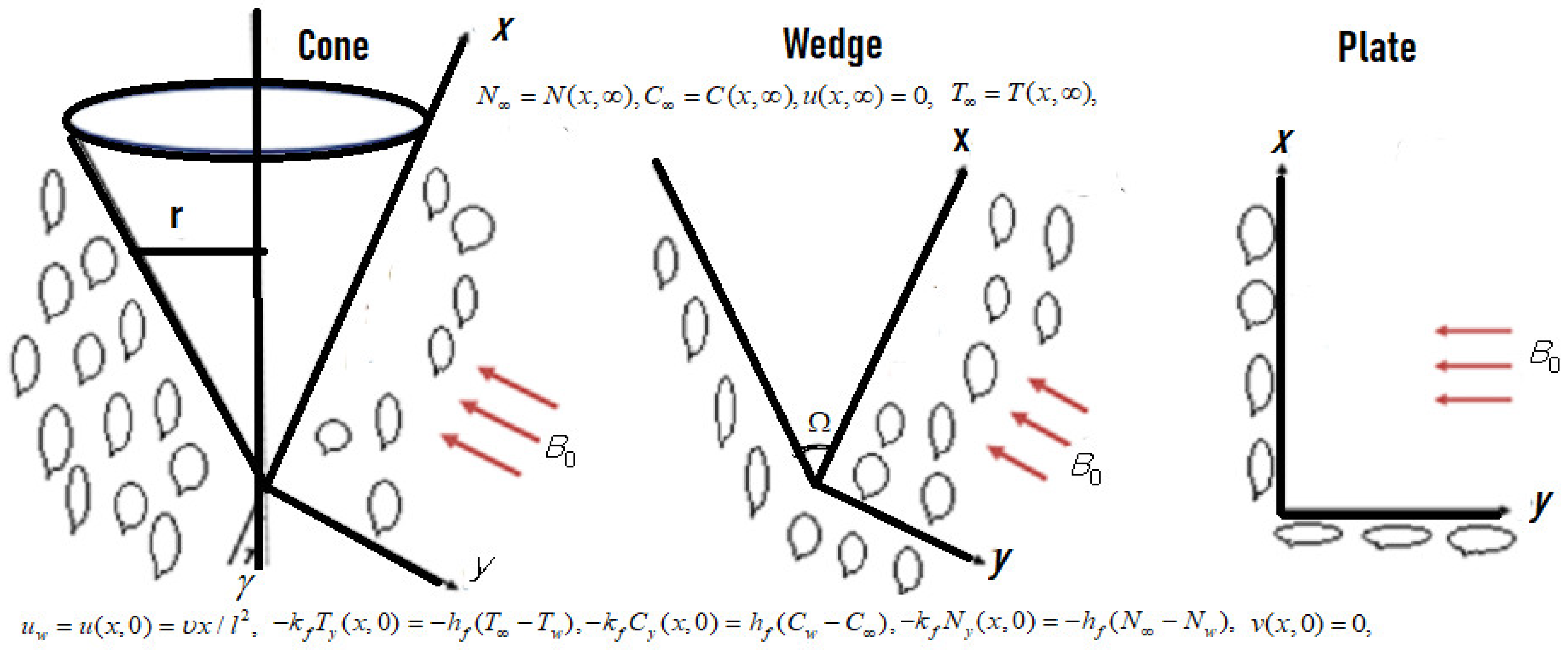
Here, an incompressible, laminar, bioconvective, electrically conducting fluid is considered over nonhomogeneous geometries ($m=0 \mathrm{and} \gamma \ne 0$, $m=0 \mathrm{and} m=0$, $m=0 \mathrm{and} \gamma \ne 0$). Let the direction of flow be in the direction of the $x$-axis, where the $y$-axis is orthogonal to it. A uniform magnetic field $B_0$ acting normal to the surface shown in Figure 1. Let the cone or wedge half angle be denoted as $\gamma$, the wedge full angle as $\mathsf{\Omega }$, and the cone radius as $r$. The whole physical system is then subjected to the non-Fourier heat flux model. The concentration and temperature close to the surface are taken as $T_w,C_w$ and $N_w$, respectively. $T_{\infty },C_{\infty } \mathrm{and} N_{\infty }$ are the ambient temperature and concentrations, respectively. Heat radiation, chemical reaction, thermophoresis, and Brownian motion impressions are considered, while the magnetic field and viscous degeneracy impressions are discarded. Raju et al. [26], Amit and Shalini [28] and Atul Kumar et al. [27].

By the Boussinesq approximation, we consider the following:

$$\frac{\partial }{\partial x}\left(\frac{u}{r^{-m}}\right)+\frac{\partial }{\partial y}\left(\frac{v}{r^{-m}}\right)=0,$$

(1)

$$u{u}_x+v{u}_y-x\left(g(T-T_{\infty }){\beta }_T+g(C-C_{\infty }){\beta }_C\right)\cos \gamma =\upsilon \left(1+\frac{1}{\beta }\right)u_{yy}-\frac{\sigma B_0{}^2}{\rho }u,$$

(2)

$$u{T}_x+v{T}_y+\delta \left(\begin{array}{l}v{u}_y{T}_x+u{u}_x{T}_x-v{u}_x{T}_y+\\ 2uv{T}_{xy}+T_{xx}{u}^2+T_{yy}{v}^2\end{array}\right)=\left(\frac{k}{\rho c_p}+\frac{16{\sigma }^{\ast }{T}_{\infty }{}^3}{3k^{\ast }}\right)T_{yy}+\tau \left(D_B{T}_y{C}_y+\frac{D_B}{T_{\infty }}{\left(T_y\right)}^2\right)$$

(3)

$$u{C}_x+v{C}_y=D_m{C}_{yy}+T_{yy}\frac{D_T}{T_{\infty }}+k_l(C+C_{\infty }),$$

(4)

$$u{N}_x+v{N}_y=N_{yy}{D}_n-\frac{b{W}_c}{\Delta C}\left(N_y{C}_y+C_{yy}\right),$$

(5)

The corresponding limitations at the boundary are:

$$\begin{gathered} u_w=u(x,0)=\upsilon x/l^2,v(x,0)=0,-k_f{T}_y(x,0)=-h_f(T_{\infty }-T_w),-k_f{C}_y(x,0)=h_f(C_w-C_{\infty }), \\ -k_f{N}_y(x,0)=-h_f(N_{\infty }-N_w),T_{\infty }=T(x,\infty ),N_{\infty }=N(x,\infty ),C_{\infty }=C(x,\infty ),u(x,\infty )=0, \end{gathered}$$

(6)

This problem involves dissimilar geometries with the following assumptions:

(i)

$\gamma \ne 0 \mathrm{and} m=0$—relates flow across a vertical wedge.

(ii)

$\gamma \ne 0 \mathrm{and} m=1$—relates flow across a vertical cone.

(iii)

$\gamma =0 \mathrm{and} m=0$—relates flow across a vertical plate.

We can now set up the similarity transformation as:

$$\begin{gathered} \frac{1}{\zeta }=\frac{l}{y},u=\frac{x\upsilon }{l^2}{f}_{\zeta },v=f(\zeta )\left[\frac{-\upsilon (1+m)}{l},\right] \\ T=T_{\infty }-\theta (\zeta )(T_{\infty }-T_w),C=C_{\infty }-\varphi (\zeta )(C_{\infty }-C_w),N=N_{\infty }+(N_w-N_{\infty })\chi (\zeta ), \end{gathered}$$

(7)

By substituting Equation (7) in Equations (1)–(4), we obtain the following equations:

$$f_{\zeta \zeta \zeta }+(1+m)f{f}_{\zeta \zeta }-f_{\zeta }{}^2-M{f}_{\zeta }+\cos \gamma \left(Gc\varphi +Gr\theta \right)=0,$$

(8)

$$\left(\frac{1}{\mathrm{Pr}}+\frac{4}{3}\frac{R}{\mathrm{Pr}}\right){\theta }_{\zeta \zeta }+{\theta }_{\zeta }{}^{2}Nt+(1+m)f{\theta }_{\zeta }+Nb{\theta }_{\zeta }{\varphi }_{\zeta }={(1+m)}^2\beta \left({\theta }_{\zeta }{f}_{\zeta }+f^2{\theta }_{\zeta \zeta }\right),$$

(9)

$$\frac{1}{Le}{\varphi }_{\zeta \zeta }-\left(Kr\varphi -(1+m)f{\varphi }_{\zeta }\right)+\frac{Nt}{Nb}{\theta }_{\zeta \zeta }=0,$$

(10)

$$\frac{1}{Le}{\chi }_{\zeta \zeta }-Pe\left({\varphi }_{\zeta }{\chi }_{\zeta }+{\varphi }_{\zeta \zeta }\left({\beta }_1+\chi \right)\right)+(m+1)f{\chi }_{\zeta }=0,$$

(11)

The analogous boundary limitations are:

$$\left.\begin{array}{l}f=0,f_{\zeta }=1,{\theta }_{\zeta }=Bi\left(\theta (\varsigma )-1\right),{\varphi }_{\zeta }=Bi\left(\varphi (\varsigma )-1\right),{\chi }_{\zeta }=Bi\left(\varphi (\varsigma )-1\right), at \zeta =0,\\ f_{\zeta }=\theta =\varphi =\chi =0 as \zeta \to \infty ,\end{array}\right\}$$

(12)

where

$$\left.\begin{array}{l}M=\frac{{\sigma }_0{B}_0{}^2{l}^2}{\rho \upsilon },Gr=\frac{l^{2}g{\beta }_T(T_w-T_{\infty })}{\upsilon u_w},Gc=\frac{l^{2}g{\beta }_C(C_w-C_{\infty })}{\upsilon u_w},\mathrm{Pr}=\frac{\mu c_p}{k},Le=\frac{\upsilon }{D_B},Bi=\frac{h_{f}l}{k_f},Pe=\frac{b{W}_c}{D_n}\\ Nb=\frac{-D_B\tau (C_{\infty }-C_w)}{\nu },Nt=\frac{-\tau D_T(T_{\infty }-T_w)}{\nu T_{\infty }},R=\frac{4{\sigma }^{\ast }{T}_{\infty }{}^3}{k{k}^{\ast }},\tau =\frac{{(\rho c_P)}_p}{{(\rho c_P)}_f},\mathsf{\Lambda }=\frac{\delta \upsilon }{l^2},Kr=\frac{k_l{l}^2}{\upsilon },{\beta }_1=\frac{N}{N-N_{\infty }}\end{array}\right\}$$

(13)

The friction factor ($C_f$), local Nusselt number ($Nu$), and local Sherwood number ($Sh$) are given by:

$$\begin{array}{l}\frac{C_f{}^{\ast }}{\mu u_w}=f″(0)\left(\frac{1}{\beta }+1\right)\\ Nu=\frac{hl}{k(T_w-T_{\infty })}=-{\theta }^{\prime }(0)\\ Sh=\frac{h_{m}l}{(C_w-C_{\infty })}=-\varphi \prime (0)\\ Sh=\frac{h_{m}l}{(N_w-N_{\infty })}=-\chi \prime (0),\end{array}$$

(14)

where $C_f{}^{\ast }$ is the dimensional wall shear stress.

3. Numerical Solutions

The nonlinear ordinary differential equations (ODEs) (8)–(11) with the boundary limitations in (12) can be numerically solved using the Runge–Kutta with shooting method. In the beginning, the set of nonlinear ODEs are transformed into first-order differential equations by the following (Raju et al. [30]) substitutions:

$$f=y_1,f^{\prime }=y_2,f^{″}=y_3,f^{‴}=y_3^{\prime },\theta =y_4,{\theta }^{\prime }=y_5,{\theta }^{″}=y_5^{\prime }=y_6,\varphi =y_7,{\varphi }^{\prime }=y_8,{\varphi }^{″}=y_8^{\prime }=y_9,\chi =y_{10}$$

$${\chi }^{\prime }=y_{11},{\chi }^{″}=y_{11}^{\prime }$$

$${y_3}^{\prime }=-(1+m)y_1{y}_3+{\left(y_2\right)}^2+m{y}_2\cos \gamma \left(Gc{y}_6+Gr{y}_4\right)$$

$${y_5}^{\prime }=\frac{-1}{\left(\frac{1}{\mathrm{Pr}}+\frac{4R}{3\mathrm{Pr}}\right)}\left[y_5{}^{2}Nt-\left(1+m\right)y_1{y}_5-Nb{y}_5{y}_7+{\left(1+m\right)}^2\beta \left(y_2{y}_5+y_1^2{y}_6\right)\right]$$

$${y_8}^{\prime }=\frac{1}{\left(\raisebox{1ex}{$1$}\!\left/ \!\raisebox{-1ex}{$Le$}\right.\right)}\left[\left(Kr{y}_7-(1+m)y_1{y}_8\right)-\frac{Nt}{Nb}{y}_6\right]$$

$${y_{11}}^{\prime }=\frac{1}{\left(\raisebox{1ex}{$1$}\!\left/ \!\raisebox{-1ex}{$Le$}\right.\right)}\left[Pe\left(y_8{y}_{10}+y_9\left({\beta }_1+y_{10}\right)\right)-\left(1+m\right)y_1{y}_{11}\right]$$

with the boundary conditions

$$y_1=0,y_2=0,y_5=Bi(y_4-1),y_8=Bi(y_7-1),y_{11}=Bi(y_{10}-1) \mathrm{at} \zeta =0$$

$$y_2={\zeta }_{1,}{y}_4={\zeta }_2,y_7={\zeta }_3,y_{10}={\zeta }_4$$

Here ${\varsigma }_1,{\varsigma }_2,{\varsigma }_3$, and ${\varsigma }_4$ are the required introductory guesses to obtain the solution. A fourth-order R-K scheme is then imposed to attain the solution. Afterward, the values of $y_2\left(\infty \right),y_4\left(\infty \right),y_7\left(\infty \right),y_{10}\left(\infty \right),$ are calculated and contrasted with the current values of the equivalent. If these are not appropriate, then the estimations of $y_3\left(0\right),y_4\left(0\right),y_6\left(0\right),y_9\left(0\right),$ are reversed to obtain a feasible solution. This procedure is repeated until a satisfactory level of precision is achieved.

4. Results and Discussion

In order to obtain the best convergence results in the graphical representation of the dimensionless velocity, temperature, concentration, and density profiles of the motile organisms, we fixed the following parameters, in addition to the friction factor and local Nusselt and Sherwood numbers:

$$Le=1,Q_H=0.2,Pe=0.5,\beta =0.2,M=0.5,\mathsf{\Lambda }=0.2,Nt=0.2,Nr=0.5,\mathrm{Pr}=5,Nb=0.3,Bi=0.2,{\beta }_1=0.2.$$

These values were stable values in our study, except for some changes that were made in the graphs.

Table 1. Variation in $f″(0)\left(1+\frac{1}{\beta }\right)$ and $-\chi \prime (0)$ for flow over a cone, wedge, and plate.

$\mathit{N}\mathit{t}$	$\mathit{N}\mathit{b}$	$\mathit{K}\mathit{r}$	$\mathit{\beta }$	$\mathit{B}\mathit{i}$	$\mathsf{\Lambda }$	${\mathit{Q}}_{\mathit{H}}$	$\mathit{N}\mathit{r}$	$\mathit{P}\mathit{e}$	$\left(1+\frac{1}{\mathit{\beta }}\right)\mathit{f}″(0)$			$-\mathit{\chi }\prime (0)$
									$\mathit{P}\mathit{l}\mathit{a}\mathit{t}\mathit{e}$	$\mathit{W}\mathit{e}\mathit{d}\mathit{g}\mathit{e}$	$\mathit{Cone}$	$\mathit{Plate}$	$\mathit{Wedge}$	$\mathit{Cone}$
0.1									−0.487683	−0.495068	−0.556183	0.159062	0.159009	0.168783
0.3									−0.479590	−0.490979	−0.555061	0.161387	0.161319	0.168960
0.5									−0.469112	−0.485634	−0.553899	0.164537	0.164476	0.169217
	0.5								−0.496125	−0.503643	−0.562239	0.160298	0.160251	0.169238
	1								−0.495968	−0.503565	−0.562421	0.159819	0.159769	0.169215
	1.5								−0.494092	−0.502618	−0.562376	0.159713	0.159656	0.169210
		0.1							−0.493197	−0.502163	−0.561736	0.160745	0.160690	0.169204
		0.3							−0.495516	−0.503337	−0.561990	0.161164	0.161119	0.169334
		0.5							−0.497066	−0.504119	−0.562194	0.161451	0.161412	0.169441
			0.1						−0.384018	−0.388781	−0.428211	0.161762	0.161735	0.169941
			0.3						−0.572366	−0.583633	−0.655850	0.160428	0.160359	0.168776
			0.5						−0.678334	−0.694246	−0.784126	0.159701	0.159601	0.168068
				0.1					−0.502091	−0.506638	−0.563330	0.088682	0.088673	0.091467
				0.2					−0.494485	−0.502816	−0.561871	0.160976	0.160927	0.169272
				0.3					−0.488400	−0.499751	−0.560598	0.222081	0.221963	0.236884
					0.1				−0.498392	−0.504777	−0.562058	0.160105	0.160068	0.169198
					0.2				−0.494485	−0.502816	−0.561871	0.160976	0.160927	0.169272
					0.3				−0.489989	−0.500571	−0.561737	0.161893	0.161825	0.169320
						0.05			−0.500451	−0.505818	−0.562223	0.158785	0.158748	0.168907
						0.1			−0.499156	−0.505168	−0.562117	0.159304	0.159263	0.169018
						0.15			−0.497328	−0.504249	−0.562000	0.159990	0.159945	0.169139
							0.5		−0.494485	−0.502816	−0.561871	0.160976	0.160927	0.169272
							1		−0.492971	−0.502050	−0.561575	0.160835	0.160780	0.169296
							1.5		−0.491706	−0.501409	−0.561280	0.160721	0.160660	0.169314
								0.5	−0.494485	−0.502816	−0.561871	0.160976	0.160927	0.169272
								1	−0.494484	−0.502816	−0.561871	0.165917	0.165885	0.171604
								1.5	−0.494484	−0.502816	−0.561871	0.170061	0.170040	0.173739

displays the changes in the friction factor coefficient and local Sherwood number in our study. The chemical reaction parameter and Peclet number were shown to encourage the mass transfer rate. Due to the dominance of mixed convection in the flow thermophoresis parameter, the Biot number, thermal relaxation, and heat generation/absorption parameters improved the collision between the particles and increased the local Sherwood number. The Brownian motion and thermal radiation parameters were correlated with declines in the local Sherwood number and increases in the friction factor coefficients. As is known, Brownian motion generates random motion in flow, which helps to improve the interaction between particles.

Table 2. Variation in ${\theta }^{\prime }(0)$ and $\varphi \prime (0)$ for flow over a cone, wedge, and plate.

$\mathit{N}\mathit{t}$	$\mathit{N}\mathit{b}$	$\mathit{K}\mathit{r}$	$\mathit{\beta }$	$\mathit{B}\mathit{i}$	$\mathsf{\Lambda }$	${\mathit{Q}}_{\mathit{H}}$	$\mathit{N}\mathit{r}$	$\mathit{P}\mathit{e}$	$-{\mathit{\theta }}^{\prime }(0)$			$-\mathit{\varphi }\prime (0)$
									$\mathit{P}\mathit{l}\mathit{a}\mathit{t}\mathit{e}$	$\mathit{W}\mathit{e}\mathit{d}\mathit{g}\mathit{e}$	$\mathit{C}\mathit{o}\mathit{n}\mathit{e}$	$\mathit{P}\mathit{l}\mathit{a}\mathit{t}\mathit{e}$	$\mathit{W}\mathit{e}\mathit{d}\mathit{g}\mathit{e}$	$\mathit{C}\mathit{o}\mathit{n}\mathit{e}$
0.1									0.232138	0.232084	0.284529	0.145565	0.145485	0.161635
0.3									0.221100	0.220981	0.282622	0.111882	0.111574	0.146700
0.5									0.205327	0.205025	0.280565	0.070846	0.069964	0.131739
	0.5								0.232168	0.232069	0.286678	0.140435	0.140333	0.159624
	1								0.213561	0.213405	0.282199	0.149395	0.149315	0.164339
	1.5								0.189804	0.189525	0.277136	0.152112	0.152026	0.165903
		0.1							0.237773	0.237670	0.288263	0.121456	0.121241	0.151256
		0.3							0.239099	0.239013	0.288380	0.133687	0.133574	0.155192
		0.5							0.240015	0.239941	0.288478	0.142013	0.141945	0.158396
			0.1						0.239030	0.239010	0.288933	0.130374	0.130302	0.154656
			0.3						0.237551	0.237373	0.287843	0.126500	0.126266	0.152344
			0.5						0.235536	0.235163	0.287116	0.123890	0.123492	0.150928
				0.1					0.141544	0.141530	0.155144	0.079212	0.079186	0.087058
				0.2					0.238506	0.238415	0.288324	0.128222	0.128070	0.153331
				0.3					0.302779	0.302537	0.401857	0.159465	0.159084	0.204679
					0.1				0.261229	0.261129	0.291949	0.133989	0.133888	0.153632
					0.2				0.238506	0.238415	0.288324	0.128222	0.128070	0.153331
					0.3				0.213788	0.213877	0.285953	0.121605	0.121423	0.153090
						0.05			0.267675	0.267658	0.292523	0.145592	0.145546	0.156996
						0.1			0.261245	0.261219	0.291257	0.141663	0.141600	0.155889
						0.15			0.252289	0.252244	0.289865	0.136290	0.136199	0.154674
							0.5		0.238506	0.238415	0.288324	0.128222	0.128070	0.153331
							1		0.316324	0.316113	0.393261	0.131375	0.131202	0.154443
							1.5		0.388685	0.388307	0.493974	0.133854	0.133666	0.155272
								0.5	0.238506	0.238415	0.288324	0.128222	0.128070	0.153331
								1	0.238502	0.238411	0.288324	0.128221	0.128069	0.153331
								1.5	0.238502	0.238411	0.288324	0.128221	0.128069	0.153331

shows the deviations in the local Sherwood and Nusselt numbers for the motion of the fluid on a cone, plate, or wedge with distinct dimensionless physical governing parameters. The heat transfer rate and mass transfer rate increased along with rising values of the Biot number, chemical reaction, and thermal radiation parameters. It was also clearly identified that these two rates were higher in the plate and wedge cases. This was likely due to the effect of thermal and concentration buoyancy forces. Rising values of thermophoresis, Casson fluid, thermal relaxation, and heat generation were shown to affect the wedge, cone, and plate cases, while the absorption parameter minimized the local Nusselt and Sherwood numbers. However, the Brownian motion parameter decreased the local Nusselt number while improving the Sherwood number.

Figure 2, Figure 3, Figure 4, Figure 5, Figure 6, Figure 7, Figure 8, Figure 9, Figure 10, Figure 11, Figure 12, Figure 13, Figure 14, Figure 15, Figure 16, Figure 17, Figure 18, Figure 19 and Figure 20 demonstrate the deviations in the temperature, velocity, concentration, and density profiles of the motile organisms for varied values of $Nt,Nb,Kr,\beta ,Bi,\mathsf{\Lambda },Q_H,Nr \mathrm{and} Pe$.

The improved Casson parameter caused a decrease in velocity and an increase in the temperature, concentration, and motile density profile. Figure 2, Figure 3, Figure 4 and Figure 5 clarify these observations. As the Casson fluid is highly viscous in nature, the velocity profile slows down the motion of fluid and improves the density, concentration, and temperature profiles of the motile organisms. Figure 6, Figure 7 and Figure 8 show the influence of $B_i$ on the density, concentration, and temperature profiles of the motile organisms for the plate, cone, and wedge cases. The density, concentration, and temperature fields were increased with a higher magnitude of $B_i$. As expected, the convective Biot number improved the interfacial distribution between the particles. The influence of $\mathsf{\Lambda }$ on the temperature and concentration fields is shown in Figure 9 and Figure 10 for plate, cone, and wedge cases. The varied value of $\mathsf{\Lambda }$ requires more time to release energy to its adjacent material particles. Because of this, the temperature profiles were increased. It was concluded that the thermal relaxation parameter showed less influence on the cone case when compared to the plate and wedge cases. The role of $Pe$ in the density profile of the motile organisms is illustrated in Figure 11. Motile organism density decreased with rising values of $Pe$ for flow in the different cases considered. Physically raising the values of $Pe$ increased the size of the motile organisms, which helped to decrease the flow. In addition, increasing the magnitude of the $Nr$ parameter enriched the temperature field. It is a well-known fact that increasing thermal radiation generates additional heat energy in flow, which helps to encourage the flow phenomena. This is plotted in Figure 12. The deviations of $Q_H$ for the concentration and temperature profiles are illustrated in Figure 13 and Figure 14. The magnitude of $Q_H$ was related to the development of the thermal and concentration boundary layers. Moreover, $Q_H$ acted as heat generation for positive values and absorption for negative values. Figure 15, Figure 16 and Figure 17 show the influence of $Nt$ on the concentration and temperature fields for the plate, wedge, and cone cases. An increase in the value of $Nt$ caused an increase in the concentration and temperature fields and reduced the density of the motile organisms. This observation suggested that thermophoresis increased the diffusion of the nanoparticles. Figure 18 and Figure 19 show the impact of $Nb$ on the concentration and temperature fields. Here, it is clear that along with growing values of $Nb$, the temperature field increased while the concentration field decreased. This was likely because the different particles had dissimilar magnitudes of $Nb$. Due to the high interfacial mass transfer in flow, the concentration profiles were decreased with increasing values of the chemical reaction parameter. This is plotted in Figure 20.

Figure 2. $\beta$ vs. $f\prime \left(\zeta \right)$.

Figure 2. $\beta$ vs. $f\prime \left(\zeta \right)$.

Figure 3. $\beta$ vs. $\theta \left(\zeta \right)$.

Figure 3. $\beta$ vs. $\theta \left(\zeta \right)$.

Figure 4. $\beta$ vs. concentration field.

Figure 4. $\beta$ vs. concentration field.

Figure 5. $\beta$ vs. density of motile organisms’ field.

Figure 5. $\beta$ vs. density of motile organisms’ field.

Figure 6. $Bi$ vs. $\theta \left(\zeta \right)$.

Figure 6. $Bi$ vs. $\theta \left(\zeta \right)$.

Figure 7. $\beta$ vs. $\varphi \left(\zeta \right)$.

Figure 7. $\beta$ vs. $\varphi \left(\zeta \right)$.

Figure 8. $\beta$ vs. $\chi \left(\zeta \right)$.

Figure 8. $\beta$ vs. $\chi \left(\zeta \right)$.

Figure 9. $\mathsf{\Lambda }$ vs. $\theta \left(\zeta \right)$.

Figure 9. $\mathsf{\Lambda }$ vs. $\theta \left(\zeta \right)$.

Figure 10. $\mathsf{\Lambda }$ vs. $\varphi \left(\zeta \right)$.

Figure 10. $\mathsf{\Lambda }$ vs. $\varphi \left(\zeta \right)$.

Figure 11. $Pe$ vs. $\chi \left(\zeta \right)$.

Figure 11. $Pe$ vs. $\chi \left(\zeta \right)$.

Figure 12. $Nr$ vs. $\theta \left(\zeta \right)$.

Figure 12. $Nr$ vs. $\theta \left(\zeta \right)$.

Figure 13. $Q_H$ vs. $\theta \left(\zeta \right)$.

Figure 13. $Q_H$ vs. $\theta \left(\zeta \right)$.

Figure 14. $Q_H$ vs. $\varphi \left(\zeta \right)$.

Figure 14. $Q_H$ vs. $\varphi \left(\zeta \right)$.

Figure 15. $Nt$ vs. $\theta \left(\zeta \right)$.

Figure 15. $Nt$ vs. $\theta \left(\zeta \right)$.

Figure 16. $Nt$ vs. $\varphi \left(\zeta \right)$.

Figure 16. $Nt$ vs. $\varphi \left(\zeta \right)$.

Figure 17. $Nt$ vs. $\chi \left(\zeta \right)$.

Figure 17. $Nt$ vs. $\chi \left(\zeta \right)$.

Figure 18. $Nb$ vs. $\theta \left(\zeta \right)$.

Figure 18. $Nb$ vs. $\theta \left(\zeta \right)$.

Figure 19. $Nb$ vs. $\varphi \left(\zeta \right)$.

Figure 19. $Nb$ vs. $\varphi \left(\zeta \right)$.

Figure 20. $Kr$ vs. $\varphi \left(\zeta \right)$.

Figure 20. $Kr$ vs. $\varphi \left(\zeta \right)$.

5. Conclusions

The addition of gyrotactic microorganisms to the Cattaneo–Christov heat flux model has many important applications in engineering, the petroleum industry, and nuclear security processes. Due to its importance, we analyzed the flow of a radiative Casson nanofluid over a cone, plate, and wedge with gyrotactic microorganisms using the Cattaneo–Christov heat flux model. Here, the variation in the different dimensionless parameters was presented graphically and in a tabular form. We also compared recently published solutions with our study and found they were in agreement. It was shown that due to the enrichment of mixed convection, the rate of mass and heat transfer was lower during flow over a plate and wedge when contrasted with flow over a cone. The heat source/sink parameter and thermal radiation parameters increased the temperature field for all the three cases. The Peclet number was found to control the mass transfer profiles for the cone, plate, and wedge cases. Finally, we concluded that the gyrotactic microorganisms played a role in enhancing the local Sherwood number.

References

1. Wilkinson, W.L. Non-Newtonian Fluids; Pergamon: New York, NY, USA, 1960. [Google Scholar]
2. Bird, R.B.; Stewart, W.E.; Lightfoot, E.N. Transport Phenomena; Wiley: New York, NY, USA, 1960; pp. 94–95. [Google Scholar]
3. Walawender, W.P.; Chen, T.Y.; Cala, D.F. An approximate Casson fluid model for tube flow of blood. Biorheology 1975, 12, 111–119. [Google Scholar] [CrossRef] [PubMed]
4. Hill, N.A.; Pedley, T.J. Bioconvection. Fluid Dyn. Res. 2005, 37, 1–20. [Google Scholar] [CrossRef]
5. Kuznetsov, A. Bio-thermal convection induced by two different species of microorganisms. Int. Commun. Heat Mass Transf. 2011, 38, 548–553. [Google Scholar] [CrossRef]
6. Tham, L.; Nazar, R.; Pop, I. Steady mixed convection flow on a horizontal circular cylinder embedded in a porous medium filled by a nanofluid containing gyro tactic micro-organisms. J. Heat Transf. 2013, 135, 102601. [Google Scholar] [CrossRef]
7. Shah, N.A.; Wakif, A.; El-Zahar, E.R.; Ahmad, S.; Yook, S.-J. Numerical simulation of a thermally enhanced EMHD flow of a heterogeneous micropolar mixture comprising (60%)-ethylene glycol (EG), (40%)-water (W), and copper oxide nanomaterials (CuO). Case Stud. Therm. Eng. 2022, 35, 102046. [Google Scholar] [CrossRef]
8. Raees, A.; Xu, H.; Liao, S. Unsteady mixed nano-bio convection flow in a horizontal channel with is upper plate expanding or contracting. Int. J. Heat Mass Transf. 2015, 86, 174–182. [Google Scholar] [CrossRef]
9. Raju, C.S.K.; Jayachandrababu, M.; Sandeep, N. Chemically reacting raidiative MHD Jeffery nanofluid flow over a cone in porous medium. Int. J. Eng. Res. Afr. 2016, 19, 75–90. [Google Scholar] [CrossRef]
10. Raju, C.; Sandeep, N. Heat and mass transfer in MHD non-Newtonian bio-convection flow over a rotating cone/plate with cross diffusion. J. Mol. Liq. 2016, 215, 115–126. [Google Scholar] [CrossRef]
11. Khan, S.U.; Al-Khaled, K.; Aldabesh, A.; Awais, M.; Tlili, I. Bioconvection flow in accelerated couple stress nanoparticles with activation energy: Bio-fuel applications. Sci. Rep. 2021, 11, 3331. [Google Scholar] [CrossRef]
12. Sajjan, K.; Shah, N.A.; Ahammad, N.A.; Raju, C.S.K.; Kumar, M.D.; Weera, W. Nonlinear Boussinesq and Rosseland approximations on 3D flow in an interruption of Ternary nanoparticles with various shapes of densities and conductivity properties. AIMS Math. 2022, 7, 18416–18449. [Google Scholar] [CrossRef]
13. Cattaneo, C. Sullaconduzionedelcalore. AttidelS Eminario Mat. Dell Univ. Modenae ReggioEmilia 1948, 3, 83–101. [Google Scholar]
14. Christov, C.I. On frame in different formulation of the Maxwell–Cattaneo model of finite-speed heat conduction. Mech. Res. Commun. 2009, 36, 481–486. [Google Scholar] [CrossRef]
15. Straughan, B. Thermal convection with the Cattaneo–Christov model. Int. J. Heat Mass Transf. 2010, 53, 95–98. [Google Scholar] [CrossRef]
16. Hayat, T.; Imtiaz, M.; Alsaedi, A.; Almezal, S. On Cattaneo–Christov heat flux in MHD flow of Oldroyd-B fluid with homogeneous–heterogeneous reactions. J. Magn. Magn. Mater. 2016, 401, 296–303. [Google Scholar] [CrossRef]
17. Rubab, K.; Mustafa, M. Cattaneo-Christov Heat Flux Model for MHD Three-Dimensional Flow of Maxwell Fluid over a Stretching Sheet. PLoS ONE 2016, 11, e0153481. [Google Scholar] [CrossRef] [PubMed]
18. Salahuddin, T.; Malik, M.; Hussain, A.; Bilal, S.; Awais, M. MHD flow of Cattanneo–Christov heat flux model for Williamson fluid over a stretching sheet with variable thickness: Using numerical approach. J. Magn. Magn. Mater. 2016, 401, 991–997. [Google Scholar] [CrossRef]
19. Hayat, T.; Farooq, M.; Alsaedi, A.; Al-Solamy, F. Impact of Cattaneo-Christov heat flux in the flow over a stretching sheet with variable thickness Impact of Cattaneo-Christov heat flux in the flow over a stretching sheet with variable thickness. Aip Adv. 2016, 5, 087159. [Google Scholar] [CrossRef]
20. Kumar, B.R.; Sivaraj, R. Heat and mass transfer in MHD viscoelastic fluid flow over a vertical cone and flat plate with variable viscosity. Int. J. Heat Mass Transf. 2013, 56, 370–379. [Google Scholar] [CrossRef]
21. Sivaraj, R.; Kumar, B.R. Viscoelastic fluid flow over a moving vertical cone and flat plate with variable electric conductivity. Int. J. Heat Mass Transf. 2013, 61, 119–128. [Google Scholar] [CrossRef]
22. Vajravelu, K.; Nayfeh, J. Hydromagnetic convection at a cone and a wedge. Int. Commun. Heat Mass Transf. 1992, 19, 701–710. [Google Scholar] [CrossRef]
23. Lou, Q.; Ali, B.; Rehman, S.U.; Habib, D.; Abdal, S.; Shah, N.A.; Chung, J.D. Micropolar Dusty Fluid: Coriolis Force Effects on Dynamics of MHD Rotating Fluid When Lorentz Force Is Significant. Mathematics 2022, 10, 2630. [Google Scholar] [CrossRef]
24. Ashraf, M.Z.; Rehman, S.U.; Farid, S.; Hussein, A.K.; Ali, B.; Shah, N.A.; Weera, W. Insight into Significance of Bioconvection on MHD Tangent Hyperbolic Nanofluid Flow of Irregular Thickness across a Slender Elastic Surface. Mathematics 2022, 10, 2592. [Google Scholar] [CrossRef]
25. Elnaqeeb, T.; Shah, N.A.; Mirza, I.A. Natural convection flows of carbon nanotubes nanofluids with Prabhakar-like thermal transport. Math. Methods Appl. Sci. 2020, 1–14. [Google Scholar] [CrossRef]
26. Raju, C.S.K.; Sandeep, N.; Lorenzini, G.; Ahmadi, M.H. Chemically reacting Carreau fluid in a suspension of convective conditions over three geometries with Cattaneo-Christov heat flux model Chemically reacting Carreau fluid in a suspension of convective conditions over three geometries with Cattaneo-Christov heat flux model. Math. Model. Eng. Probl. 2018, 5, 293–302. [Google Scholar] [CrossRef]
27. Kumar, R.A.; Vasu, B.; Bég, O.A.; Gorla, R.S.R.; Murthy, P.V.S.N. Homotopy semi-numerical modeling of non-Newtonian nanofluid transport external to multiple geometries using a revised Buongiorno Model. Inventions 2019, 4, 54. [Google Scholar]
28. Parmar, A.; Jain, S. Influence of Non-Linear Chemical Reaction on MHD Convective Flow for Maxwell Fluid Over Three Different Permeable Vertical Surfaces. J. Nanofluids 2019, 8, 671–682. [Google Scholar] [CrossRef]
29. Chaurasiya, V.; Wakif, A.; Shah, N.A.; Singh, J. A study on cylindrical moving boundary problem with variable thermal conductivity and convection under the most realistic boundary conditions. Int. Commun. Heat Transf. 2022, 138, 106312. [Google Scholar] [CrossRef]
30. Raju, C.; Khan, I.; Raju, S.; Upadhya, M. Micro and Nanofluid Convection with Magnetic Field Effects for Heat and Mass Transfer Applications Using MATLAB®, 1st ed.; Elsevier: Amsterdam, The Netherlands, 2022; ISBN 9780128231418. [Google Scholar]
Figure 1. Physical representation.
Mathematics 10 03508 g001