
Identification of Location and Camera Parameters for Public Live Streaming Web Cameras


Abstract

1. Introduction
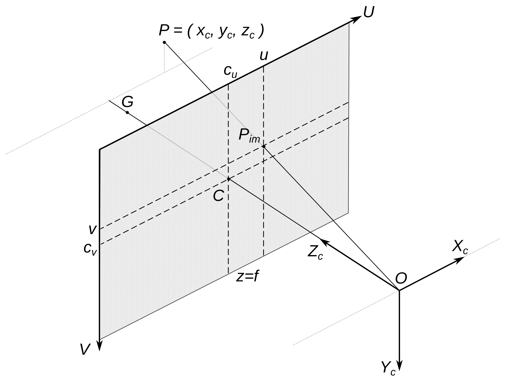
2. Coordinate Systems, Models
3. Public Camera Parameters Estimation
Site-Specific Calibration
4. Formulation of the Problem and Its Solution Algorithm
- Let Q be the area that is a plane section of the road surface in space (the road plane can be inclined);
- Φ is the camera frame of resolution containing the image of Q, denoting the image by ;
- Φ contains the image of at least one segment, the prototype of which in space is a segment of a straight line with a known slope (e.g., vertical);
- The image is centered relative to the optical axis of the video camera, that is, and ;
- The coordinates of the points O (camera position) and G (the source of the optical center C) are known;
- The coordinates of one or more pixels of located on the line and the coordinates of their sources are known;
- The coordinates of one or more pixels of located on the line and the coordinates of their sources are known;
- The coordinates of three or more points are known; at least three of them must be non-collinear;
- The coordinates of one or more groups of three pixels are known, and in the group, the sources of the pixels are collinear in space.
4.1. Solution Algorithm
4.1.1. Obtain the Intrinsic Parameters (Matrix A)
4.1.2. Obtain the Radial Distortion Compensation Map
4.1.3. Obtain the Camera Orientation (Matrix R )
4.1.4. Obtain the Mapping for
4.2. Auxiliary Steps
4.2.1. Describing of the Area Q
4.2.2. Coordinate Frame Associated with the Plane
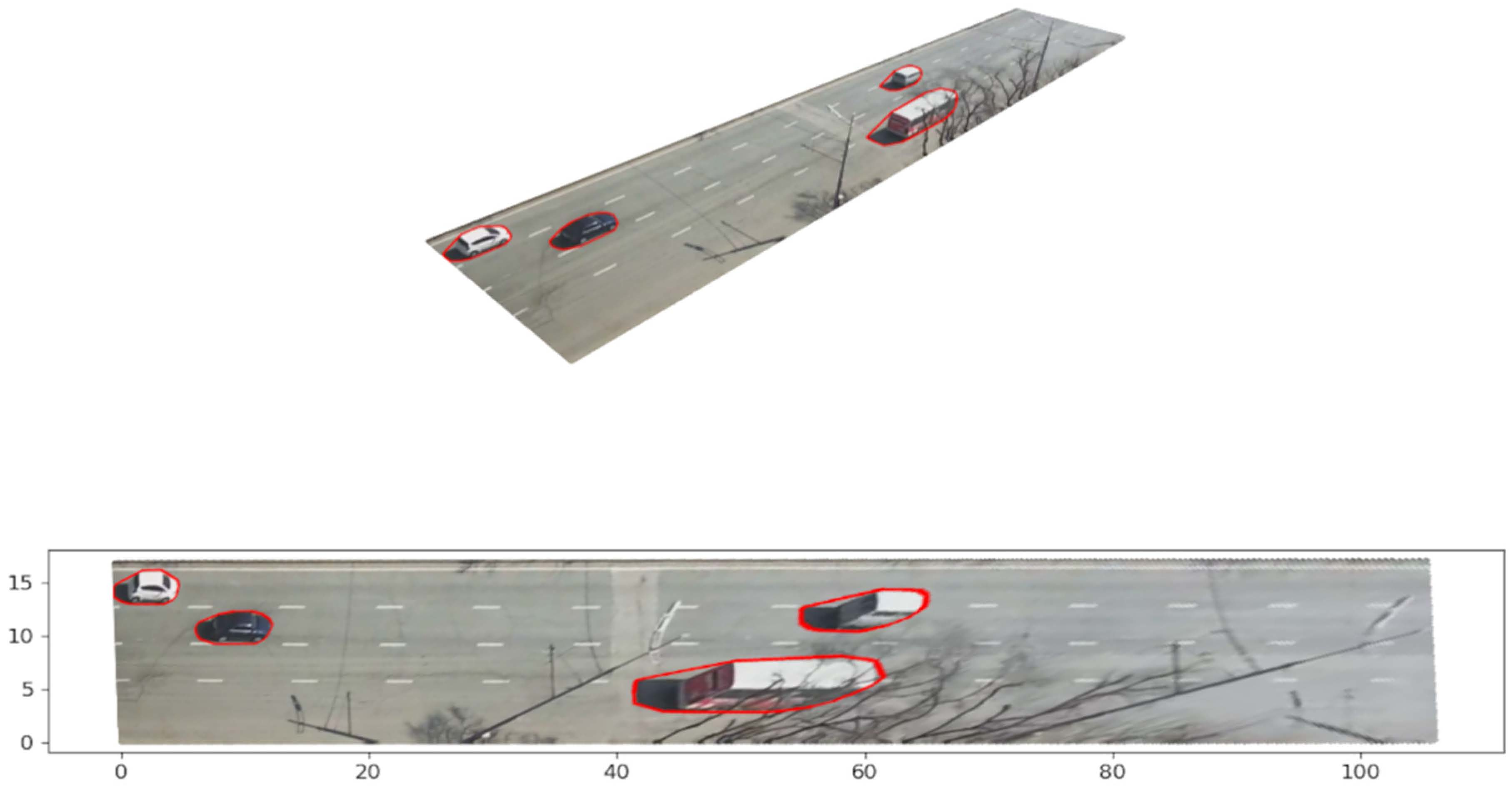
5. Examples
5.1. Example 1: Inclined Driving Surface and a Camera with Tilted Horizon
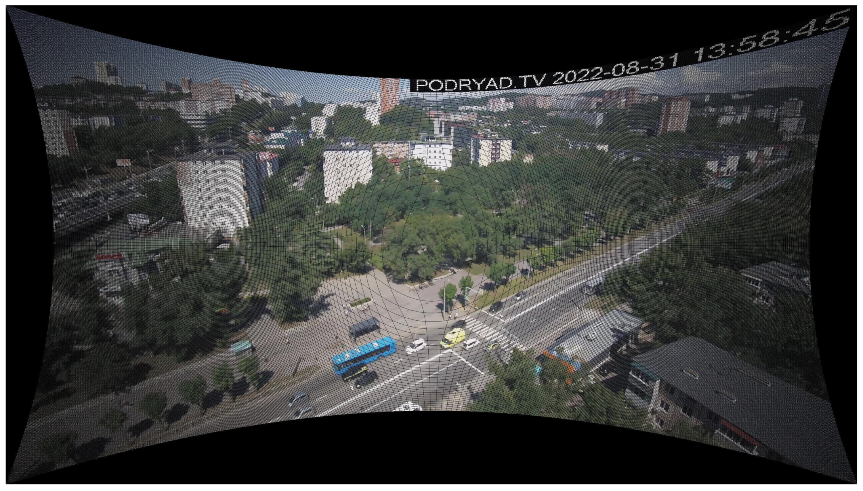
5.2. Example 2. More Radial Distortion and Vegetation, More Calibration Points
6. Conclusions
Author Contributions
Funding
Data Availability Statement
Conflicts of Interest
References
- Xinqiang, C.; Shubo, W.; Chaojian, S.; Yanguo, H.; Yongsheng, Y.; Ruimin, K.; Jiansen, Z. Sensing Data Supported Traffic Flow Prediction via Denoising Schemes and ANN: A Comparison. IEEE Sens. J. 2020, 20, 14317–14328. [Google Scholar]
- Xiaohan, L.; Xiaobo, Q.; Xiaolei, M. Improving Flex-route Transit Services with Modular Autonomous Vehicles. Transp. Res. Part E Logist. Transp. Rev. 2021, 149, 102331. [Google Scholar]
- 75 Years of the Fundamental Diagram for Traffic Flow Theory: Greenshields Symposium TRB Transportation Research Electronic Circular E-C149. 2011. Available online: http://onlinepubs.trb.org/onlinepubs/circulars/ec149.pdf (accessed on 17 September 2022).
- Zatserkovnyy, A.; Nurminski, E. Neural network analysis of transportation flows of urban agglomeration using the data from public video cameras. Math. Model. Numer. Simul. 2021, 13, 305–318. [Google Scholar]
- Camera Calibration and 3D Reconstruction. OpenCV Documentation Main Modules. Available online: https://docs.opencv.org/4.5.5/d9/d0c/group__calib3d.html (accessed on 18 March 2022).
- Szeliski, R. Computer Vision: Algorithms and Applications, 2nd ed.; Springer: Cham, Switzerland, 2022. [Google Scholar]
- Hartley, R.; Zisserman, A. Multiple View Geometry in Computer Vision, 2nd ed.; Cambridge University Press: New York, NY, USA, 2003. [Google Scholar]
- Transformations between ECEF and ENU Coordinates. ESA Naupedia. Available online: https://gssc.esa.int/navipedia/index.php/Transformations_between_ECEF_and_ENU_coordinates (accessed on 18 March 2022).
- Forsyth, D.A.; Ponce, J. Computer Vision: A Modern Approach, 2nd ed.; Pearson: Hoboken, NJ, USA, 2012. [Google Scholar]
- Peng, S.; Sturm, P. Calibration Wizard: A Guidance System for Camera Calibration Based on Modeling Geometric and Corner Uncertainty. arXiv 2019, arXiv:1811.03264. [Google Scholar]
- Camera Calibration. OpenCV tutorials, Python. Available online: http://docs.opencv.org/4.x/dc/dbb/tutorial_py_calibration.html (accessed on 18 March 2022).
- Marchand, E.; Uchiyama, H.; Spindler, F. Pose estimation for augmented reality: A hands-on survey. IEEE Trans. Vis. Comput. Graph. 2016, 22, 2633–2651. [Google Scholar] [CrossRef] [PubMed]
- Perspective-n-Point (PnP) Pose Computation. OpenCV documentation. Available online: https://docs.opencv.org/4.x/d5/d1f/calib3d_solvePnP.html (accessed on 18 March 2022).
- Liu, C.-M.; Juang, J.-C. Estimation of Lane-Level Traffic Flow Using a Deep Learning Technique. Appl. Sci. 2021, 11, 5619. [Google Scholar] [CrossRef]
- Khazukov, K.; Shepelev, V.; Karpeta, T.; Shabiev, S.; Slobodin, I.; Charbadze, I.; Alferova, I. Real-time monitoring of traffic parameters. J. Big Data 2020, 7, 84. [Google Scholar] [CrossRef]
- Zhengxia, Z.; Zhenwei, S. Object Detection in 20 Years: A Survey. arXiv 2019, arXiv:1905.05055v2. [Google Scholar]
- Huchuan, L.; Dong, W. Online Visual Tracking; Springer: Singapore, 2019. [Google Scholar]
- Yandex Maps. Available online: https://maps.yandex.ru (accessed on 18 March 2022).


| Name | Lat | Long | Height | u | v | |||
|---|---|---|---|---|---|---|---|---|
| 56 | 0 | 0 | 0 | |||||
| G | 57 | 960 | 540 | 1 | ||||
| O | 98 | 42 | ||||||
| 57 | 1534 | 540 | 1 | |||||
| 52 | 960 | 353 |
| Num | Lat | Long | Height | |||
|---|---|---|---|---|---|---|
| 1 | ||||||
| 2 | 59 | |||||
| 3 | ||||||
| 4 | ||||||
| 5 | ||||||
| 6 | ||||||
| 7 | 56 | |||||
| 8 | ||||||
| 9 | 56 |
| Corner | Name | u | v |
|---|---|---|---|
| top left | 504 | 849 | |
| bottom left | 739 | 1079 | |
| top right | 1468 | 410 | |
| bottom right | 1642 | 462 |
| Name | Lat | Long | Height | u | v | |||
|---|---|---|---|---|---|---|---|---|
| 14 | 0 | 0 | 0 | |||||
| G | 25 | 960 | 540 | |||||
| O | 56 | |||||||
| 18 | 306 | 540 | ||||||
| 15 | 960 | 671 | ||||||
| 14 | 1559 | 540 | ||||||
| 960 | 815 | |||||||
| 43 | 960 | 199 |
| Num | Lat | Long | Height | |||
|---|---|---|---|---|---|---|
| 1 | ||||||
| 2 | ||||||
| 3 | 14 | |||||
| 4 | ||||||
| 6 | 15 | |||||
| 7 | 14 | |||||
| 8 | 14 | |||||
| 9 | 14 | |||||
| 10 | 14 | |||||
| 11 |
| Corner | Name | u | v |
|---|---|---|---|
| top left | 509 | 962 | |
| bottom left | 993 | 1078 | |
| top right | 1630 | 498 | |
| bottom right | 1858 | 558 |
Publisher’s Note: MDPI stays neutral with regard to jurisdictional claims in published maps and institutional affiliations. |
© 2022 by the authors. Licensee MDPI, Basel, Switzerland. This article is an open access article distributed under the terms and conditions of the Creative Commons Attribution (CC BY) license (https://creativecommons.org/licenses/by/4.0/).
Share and Cite
Zatserkovnyy, A.; Nurminski, E. Identification of Location and Camera Parameters for Public Live Streaming Web Cameras. Mathematics 2022, 10, 3601. https://doi.org/10.3390/math10193601
Zatserkovnyy A, Nurminski E. Identification of Location and Camera Parameters for Public Live Streaming Web Cameras. Mathematics. 2022; 10(19):3601. https://doi.org/10.3390/math10193601
Chicago/Turabian StyleZatserkovnyy, Aleksander, and Evgeni Nurminski. 2022. "Identification of Location and Camera Parameters for Public Live Streaming Web Cameras" Mathematics 10, no. 19: 3601. https://doi.org/10.3390/math10193601
APA StyleZatserkovnyy, A., & Nurminski, E. (2022). Identification of Location and Camera Parameters for Public Live Streaming Web Cameras. Mathematics, 10(19), 3601. https://doi.org/10.3390/math10193601