Abstract
In the context of the high dependency on fossil fuels, the strong efforts aiming to shift towards a more sustainable world are having significant economic and political impacts. The electricity market is now encouraging prosumers to consume their own production, and thus reduce grid exchanges. Self-consumption can be increased using storage systems or rescheduling the loads. This effort involves not only residential prosumers but also industrial ones. The rescheduling process is an optimisation problem that can be effectively solved with evolutionary algorithms (EAs). In this paper, a specific procedure for bridging demand-side management from the theoretical application to a practical industrial scenario was introduced. In particular, the toroidal correction was used in the differential evolution with the aim of preventing the local minima worsening the effectiveness of the proposed method. Moreover, to achieve reasonable solutions, two different cost contributions have been considered: the energy cost and the labour cost. The method was tested on real data from a historical textile factory, Ratti S.p.A. Due to the nature of the loads, the design variables were the starting time of the 30 shiftable loads. The application of this procedure achieves a reduction in the total cost of approximately 99,500 EUR/year.
MSC:
68T20
1. Introduction
In the last 10 years, Europe has made significant efforts to increase its sustainability and energy independence [1]. The goal of net zero carbon emission by 2050 has strong significance in terms of both environmental impact and economic and political struggles. In the post-COVID-19 era, the fast economic recovery of countries has changed all the energy markets’ equilibria [2]. All these factors have contributed to high variability and insecurities in the energy market, with consequently a high variability in electricity, natural gas, and oil prices. With a high dependency on fossil fuels, Europe has the environmental, economic and political imperative to become self-sufficient to the greatest extent possible and as soon as possible. With economic pressures having the greatest impact, the increase in fossil fuel and electricity prices have motivated the search for how one may pursue the diversification of energy sources [3].
Renewables are seen in this context as the main option to reduce this external energy dependency and at the same time to decrease the environmental burden associated with the use of fossil fuels. Such a strong push towards renewable energies was never seen even in the first decade of the 2000s, when European countries applied large incentives to stimulate the market of renewables. Moreover, electrification processes to disengage from the use of natural gas for heating or process uses will lead to further increases in electricity consumption which must be compensated by clean energy sources [4]. The non-programmable and non-dispatchable characteristics of renewables, however, can give rise to problems in the stability of the grid. The problems associated with the increasingly higher penetration of fluctuating productions still has to be addressed in order to better integrate them into the supply system. On the one hand, there is therefore the push towards renewables, whilst on the other hand, the electricity market, incentives and grid exchange rules are now discouraging unregulated distributed energy production. Renewables are now encouraged, but only if associated to self-consumption and with extremely low grid exchanges. In this context, prosumers are a key element that can be exploited for an effective energy transition. Prosumers are consumers that contribute to production. This is a general term which can refer to all goods, but it is specifically well-suited to the energy sector. Energy prosumers can produce part or all of the energy they use, or even excess energy. Prosumers have to deal with self-consumption and many incentives have been created to boost the birth of these actors [5,6].
There are few possibilities to increase renewable production whilst maintaining high self-consumption. One of the most diffuse methods is the use of battery storage systems. These can help in energy management, handling the peaks of production and consumption. However, they still have high costs [7]. Another emerging technology is hydrogen. Its use as a storage system can have a significant impact on the energy market and on the use of renewables; hydrogen can be produced through electrolysis exploiting the excess of renewables and this can be a strong ally of grid stability. Moreover, hydrogen can be simply stocked or transported and directly used as fuel or reconverted into electricity through fuel cells. The costs related to this process is even higher than the cost of batteries; thus, this solution is still not commercial [8]. Finally, the other way to self-consume renewables is load scheduling. This is certainly the most economical way, but not the easiest: in particular, different automated home energy management systems have been developed with the aim of helping prosumers handled their loads. These kinds of electricity management problems have already been extensively analysed, but new points of view are always possible stimuli to investigate new technologies [9].
The aim of this work was to define a viable and practical method in order to bridge all the research in residential DSM to the industrial sector. This application is a great challenge due to the additional constraints and the more complex data preprocessing required. The proposed method improves the traditional load shifting that can be found in the literature. In particular, there are two main contributions. Firstly, a specifically designed Differential Evolution (DE) with toroidal correction was used to achieve a good convergence of the algorithm and reduce the possibility of stagnation in local minima. Secondly, in order to achieve practically implementable solutions, the cost function has been designed in order to consider both the electricity price and the labour cost. This second element has been considered in order to achieve practically implementable solutions. With respect to many applications of residential DSM, in this work, the method has been applied to different scenarios. These are defined by all the measured days used in the optimisation. This is a key factor for assessing the applicability of the method. The obtained schedule should be globally optimal over different weather conditions because it cannot be easily changed during the year.
2. Related Works
Electricity management problems can be classified into two main groups, namely supply-side management (SSM) and demand-side management (DSM) [10]. The SSM consists of the actions to manage the generation, transmission, and distribution of energy, thus usually without involving prosumers. On the other hand, the DSM concerns all the activities on the side of electric utilities, such as planning, implementing, and monitoring the loads consumptions. This management can improve grid stability, but always keep a focus on the end-user comfort. Demand-side management, of course, can be applied to prosumers to improve their self-consumption, managing both the production and the loads, and the storage systems when present [11].
Demand-side management has been well studied in the literature: dynamic tariffs, real-time prices, capacity market, and demand response are some of the mechanisms that the electricity market can use to encourage a better management of the demand-side electricity usage. With renewables penetration, distributed production, and grid stability problems, this topic is increasingly urgent, and it is expected that, in the near future, some of the incentive mechanisms above will be applied [12].
Evolutionary algorithms (EAs) are powerful optimisation tools; they have been exploited in different problems related to SSM and DSM because they allow a global search in non-linear and multi-modal environments that characterise DSM [13,14].
In [15], the authors applied chaotic evolutionary programming to improve the convergence for a combined heat and power dispatch problem. The same algorithm was applied in [16] for managing the hydroelectric power generation integrated with pumping and energy management systems.
Most of the research on DSM is focused on the residential sector, in which the end-user is more involved and willing to modify its practices to reduce electricity bills, keeping a high level of user satisfaction [17,18]. Different approaches were studied for helping the development of DSM, such as price-based or incentive-based programs [19].
Several EAs have been applied in this field. Genetic algorithm and particle swarm optimisation are traditional ones that have been widely applied for managing electric vehicles loads [20], optimising micro-market strategies [21], and operating smart grids [22]. More advanced algorithms have been applied to DSM, such as biogeography-based optimisation and whale optimisation algorithm [23,24].
In general, the aim of DSM is not only the minimisation of the electricity bill, but also to keep a high end-user satisfaction. As an example, in [25] two components are included in the definition of user satisfaction: the time slot of load activation and the risk of the interruption of the energy supply due to excess in the power contracted and uncontrolled loads. In [26], the method was integrated with electric vehicles considering the state-of-charge as an additional performance parameter. In both of these papers, the problem was solved with elitist non-dominated sorting genetic algorithm II. Additional examples of the application of EAs in residential DSM can be found in [27], where the thermal load is considered, and in [28], where a specifically designed algorithm is applied to manage the thermostatically controlled loads and stationary storage system. A different approach was applied in [29], where the authors maximised the user’s satisfaction fixing the level of electricity cost. A similar problem was considered in [30], where the ecological impact was also introduced as a performance parameter.
3. Methods
The aim of the proposed method was to apply DSM techniques in an industrial scenario. This process was specifically designed to address all the criticalities that can be found in such a complex environment. The proposed method is schematically shown in Figure 1. It is divided in two main parts: the data preparation and the optimisation process.
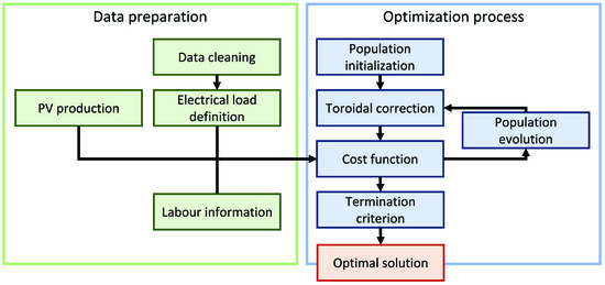
Figure 1.
Flowchart of the proposed method.
In the following, the two phases are described in details.
3.1. Data Preparation
The aim of the data preparation was to obtain the information required to compute the cost value. The first step of the data preparation is the cleaning. There are two elements that should be considered when cleaning data: Firstly, non-working days, such as weekends and holidays, when activity is reduced and no load shift can be performed; Secondly, the elimination of outliers in the data, which may be due to errors in the measurement system. This second correction is performed with a statistical analysis [31]. The outliers were identified by computing the standard deviation of the power profiles and eliminating those that are outside 3.1 times the standard deviation.
The company is composed of several electrical loads; however, only some of them are measured, and among them, 30 can be shifted. Due to the nature of the operations performed in the analysed company, no other modifications of the loads can be performed. In order to identify the time profile of the shiftable loads from the available measures, the raw data measured in the considered period were collected, the outliers were identified, and the average profile was computed:
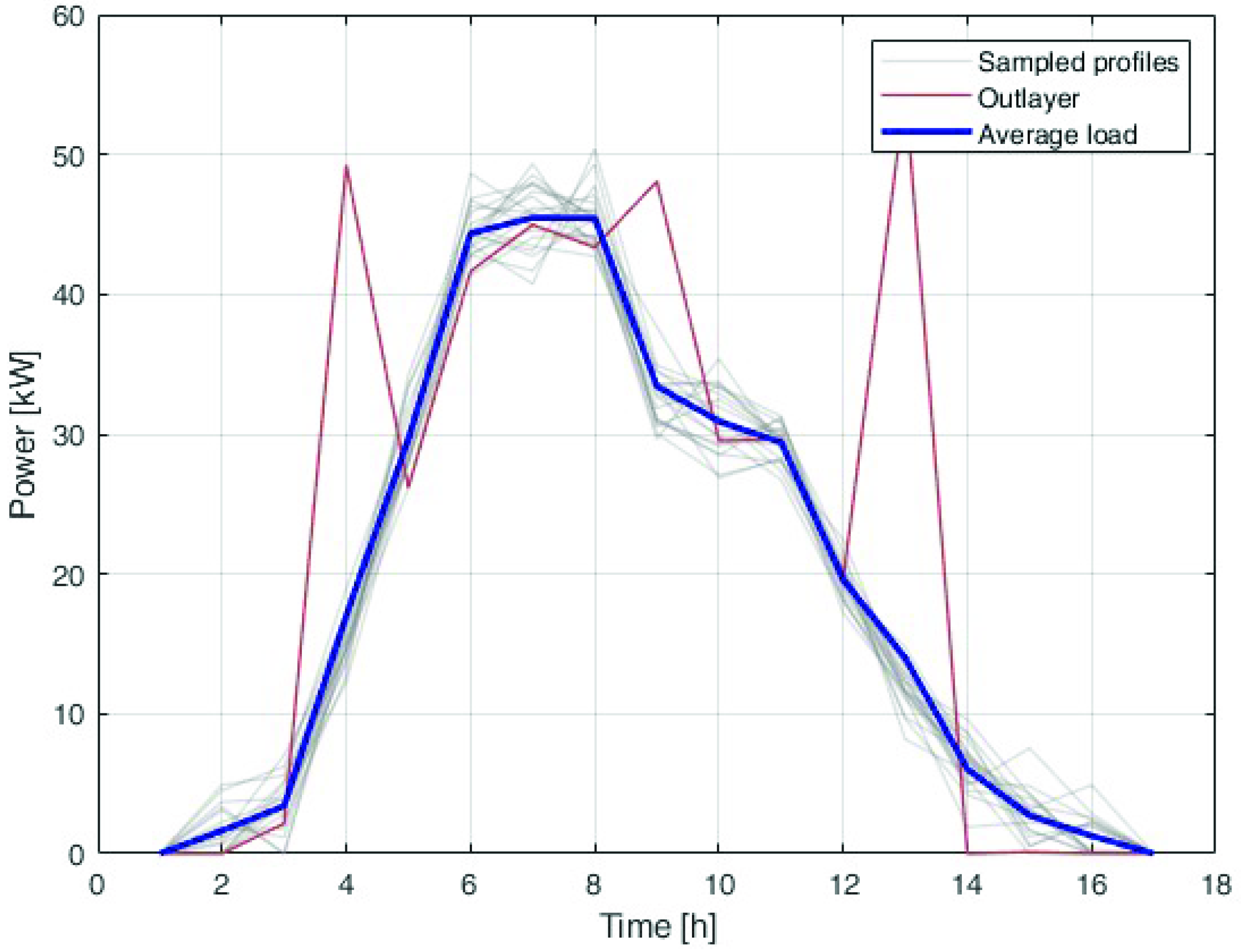
where are the number of available days of sampled data, and is the time profile of the i-th load in the k-th day. Figure 2 shows an example of the computation of the average load. Each sampled profile is shown in grey, and the red line shows an outlier, while the blue line is the average profile used in the optimisation.
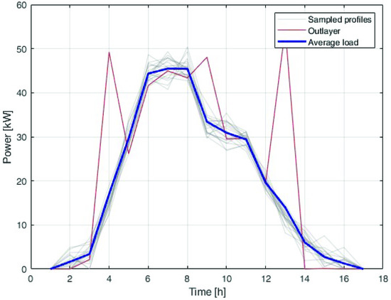
Figure 2.
Example of computation of average load. Each sampled profile is represented in grey, the red line shows an outlier, while the blue line is the average profile used in the optimisation.
The baseload used in the optimisation process for defining the different scenarios is obtained by subtracting the measured power profiles of the shiftable loads from the total load absorbed by the company:
The baseload profile is computed for all of the analysed period, and it varies from one day to another. This is very important because it allows to take into consideration the seasonality in the optimisation process, thus obtaining a robust solution. The second element required for the cost computation is the PV power production. Furthermore, in this case, the measured profile is fed as the input of the optimiser to consider the seasonality and weather variations. Finally, the third element required is the labour information related to each single load: the number of people required can change over time. This is a key factor of the proposed method: it allows to compensate the economical push toward the night-shift of the loads. All the information obtained in the data preparation phase is used in the computation of the cost function during the optimisation process.
3.2. Optimisation Process
The optimisation process implements a modification of differential evolution (DE) with toroidal correction. It is an evolutionary algorithm that shares some similarities with the genetic algorithm. It has been introduced in [32] for solving continuous optimisation problems with the aim to handle non-differentiable, nonlinear, and multimodal cost functions. Moreover, it was designed to be easy for the user (robustness of the parameters choice) and suitable for parallelisation.
The algorithm is based on the vector-based mutation: this operator has the objective to create the new population starting from the existing one. The population evolution of DE at each iteration is shown in Figure 3. As a first step, two individuals of the population are selected (all the selection possibilities can be used) and the difference vector is calculated. Then, a third individual, different from the previous ones, is selected, and it moves in the search space by a quantity that is proportional to the difference vector:

Figure 3.
Population evolution of DE at each iteration.
The design variables of this problem are the starting time for all the loads. The total load represented by a candidate solution i can be computed considering the baseload and the photovoltaic production:
where the starting time of each shiftable load is modified according to the k-th element of the i-th candidate solution.
Due to the periodic nature of the design variables, a toroidal correction was introduced to manage the search space boundary [33]. This correction means that a solution that exits the search space from one boundary is reinserted on the other side. It can be expressed in the following way:
where is the corrected i-th element of the candidate solution x, is the lower boundary for the i-th variables, and is its upper boundary.
In order to apply this methodology to a real industrial application, another performance parameter should be analysed. This is the labour cost: in fact, each activity is characterised by a certain amount of workforce required in each step. The workforce cost can be computed to create a time profile in the day, and then associating its cost to each time slot. The time profile of the workforce can be computed as follows:
where is the total workforce profile and is the one associated to the k-th load. In this cost, the workforce related to the baseload is not considered, because only the differential cost between two solutions impacts the optimisation performances.
The final objective function is the minimisation of the sum of the two cost components, the energy cost and the workforce cost. Both these cost values are influenced by the design variables, i.e., the time shift of each load; consequently, the number of design variables is equal to the number of shiftable loads. Each design variable can vary in the range .
4. Case Study
The method proposed in this paper was tested with real data from a textile company in Italy. Ratti S.p.A. is an historic and big company in the industry of Guanzate (CO). Its production consists of all the processes from the yarn to the finished fabric and, being custom tailored, it is very complex and not linear at all. Like every textile factory, Ratti is energy-intensive with an electricity consumption of approximately 8 TWh per year. The mill is connected to the national electrical grid through an electric cabinet in medium voltage (15 kV). Inside of the company, there is an MV ring to which five transformation cabinets (MV–LV) are connected.
The company has approximately 1 MW of PV installed on their buildings and another four smaller plants are in the designing phase. When the new instillations will be completed, the company will have approximately 1.5 MW of PV plants, divided in eight sub-plants, each of which characterised by a different exposure forced by the buildings geometry. These plants are connected to different cabinets, and this was considered in the following analysis. Table 1 shows the PV plants’ details: the first four sections are already installed and the last four are newly designed.

Table 1.
PV plant characteristics.
The company is provided with a monitoring system for most of the loads. In this analysis, 30 shiftable loads were considered. In addition, a base-load is considered for each cabinet: it is composed of non-programmable consumptions, and some machines that are not measured.
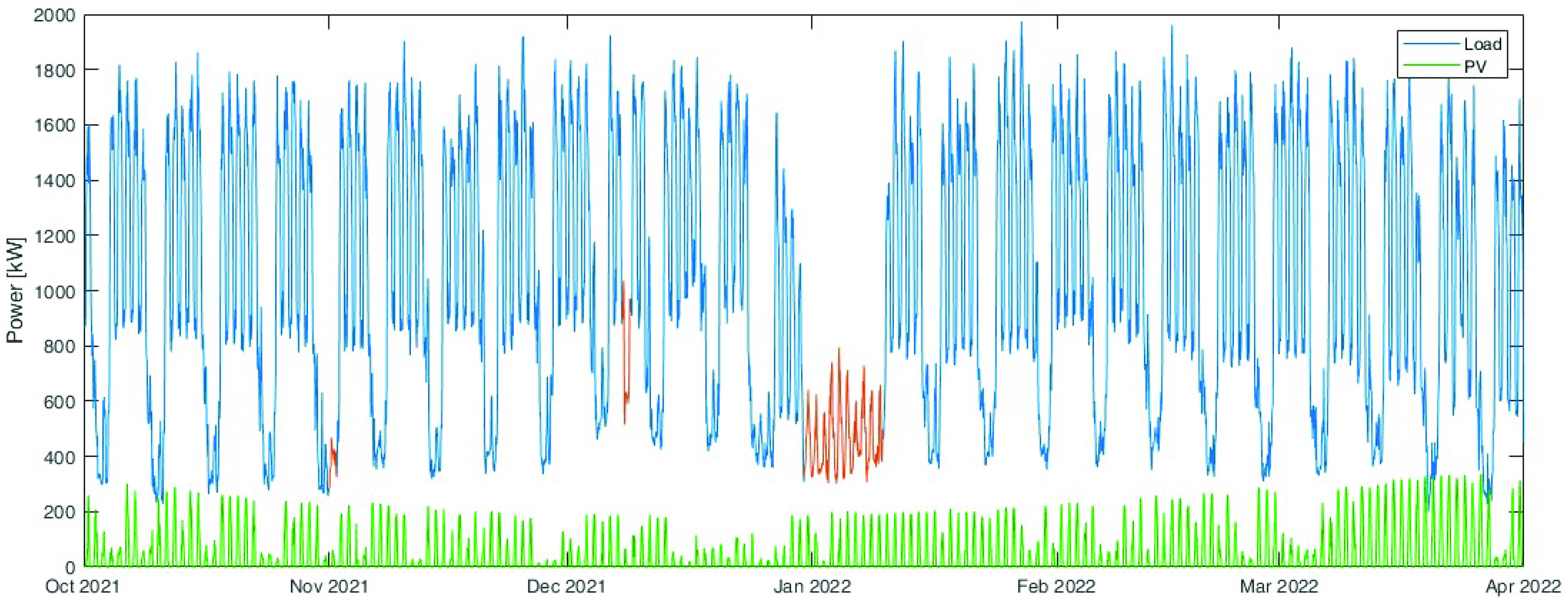
The entire analysis was performed analysing the data collected in the period from October 2021 to March 2022 with hourly data sampling. The data were preprocessed in order to eliminate the holidays and anomalies, and to obtain the values of the load that can be shifted in the optimisation process. Figure 4 shows the total load absorbed by the analysed company (in blue): the days highlighted in red are not working days; thus, they were eliminated from the analysis. In green is represented the photovoltaic power production.
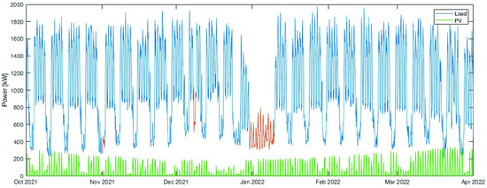
Figure 4.
Power profiles used as input for the data processing phase. In blue, the total load absorbed by the analysed company; in red, the holidays that should be eliminated in the analysis; and in green, the photovoltaic power production.
The electricity cost takes into consideration three different elements. Firstly, the energy price is characterised by two different tariffs: the peak tariff, from 8 a.m. to 8 p.m., and the off-peak tariff, from 8 p.m. to 8 a.m. The real monthly tariff is used in the optimisation. Secondly, there is a cost associated with the contracted power, i.e., the maximum power that can be absorbed by the company. Thirdly, the surplus of energy can theoretically be sold to the electrical grid, and it is paid; this has been introduced in the optimisation cost function even though it is never verified during the analysed working days.
Another key element in the definition of the electricity bill is the cost associated with the maximum power required from the network. The human resources are organised over three work shifts: 6 a.m.–2 p.m., 2 p.m.–10 p.m., and 10 p.m.–6 a.m. For the first two time slots, the average working cost was considered equal to 20 EUR/h, while in the third time slot, it was considered equal to 30 EUR/h.
5. Results
In this section, the results obtained by the proposed methodology are shown and analysed. Firstly, the preprocessing results are shown: these are used as input to the optimisation process. Then, the optimisation results are shown. In order to justify the proposed method, three different analyses were performed:
- Firstly, a basic optimisation with DE was performed only considering the electricity bill as the performance parameter. These results are used as a benchmark for the following analyses;
- Secondly, the proposed TC-DE is applied for the minimisation of the electrical bill;
- Finally, the optimisation results considering both the electricity bill and the labour cost.
5.1. Data Preprocessing
The first step in the application of the proposed DSM method in an industrial scenario is an accurate preprocessing of the data.
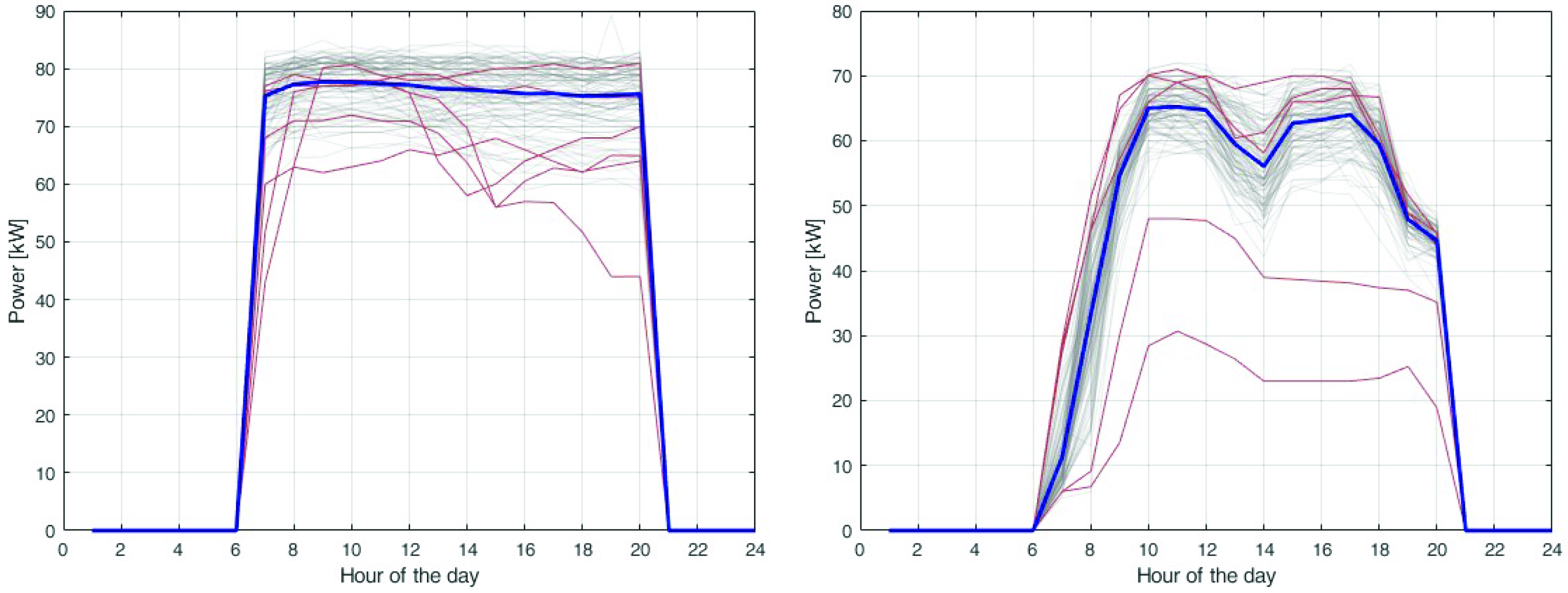
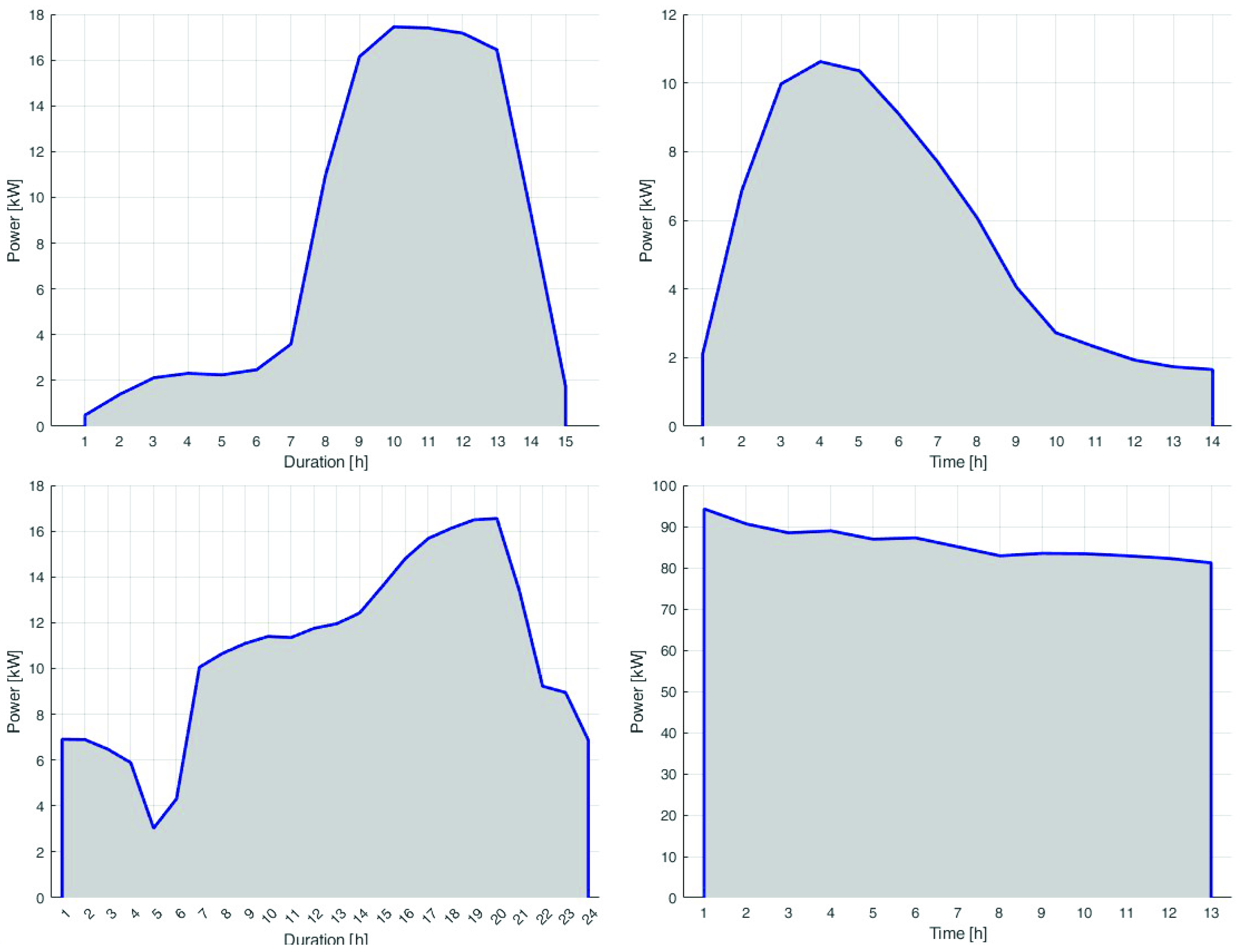
The data cleaning phase consists of the elimination of holidays and exceptions in the load profiles. When the daily profiles were cleaned, the average load is computed. Figure 5 shows the results of this phase: in grey, all 175 daily measurements of the load are shown; in red, the outliers are highlighted; and in blue, the average load is shown. With this phase, 30 average loads are identified and introduced in the optimisation process. Some examples of the loads are reported in Figure 6: the profiles are characterised by different durations, maximum power, and shape. The load duration depends on the industrial process associated with it. In particular, there are a couple of loads that last the entire day: in this case, the load shifting can be used to move the peak and the load at the most convenient time of day.

Figure 5.
Results of the data cleaning and averaging phase: in grey, all 175 daily measurements of the load are shown; in red, the outliers are highlighted; and in blue, the average load is shown.
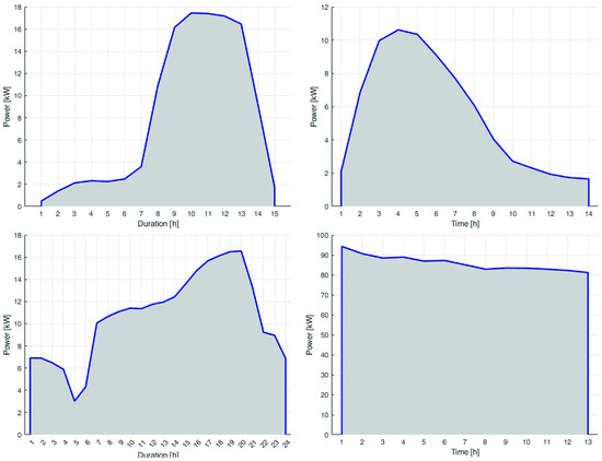
Figure 6.
Examples of shiftable loads. The x axis represents the duration of the load in hours.
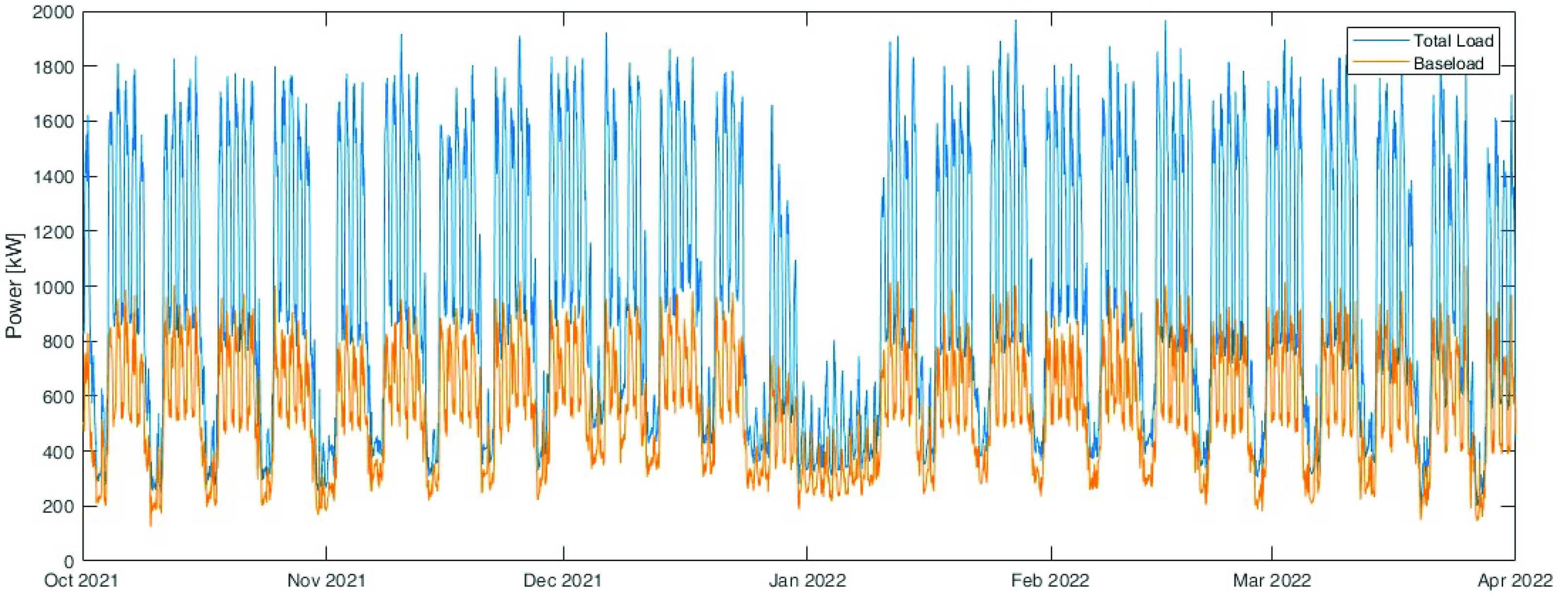
Another important aspect that should be considered in the procedure is the baseload, i.e., all the loads that cannot be managed or that have not been measured. Figure 7 shows the computed baseload (in orange) compared with the total load. The baseload correspond to the 55% of the total energy absorbed during the analysed period. Excluding holidays and weekends, the impact of the baseload is 53%.
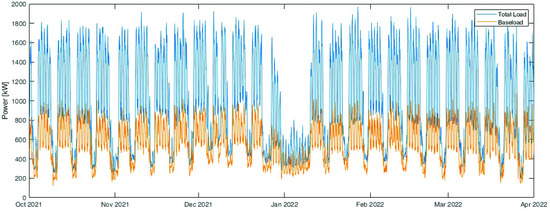
Figure 7.
Computed baseload (in orange) compared with the total load (in blue).
5.2. Base Case Optimisation
Here, a first basic optimisation is performed to have another benchmark for the results analysis. This optimisation is also used to highlight the criticality that is solved by means of the proposed method.
The optimisation was performed by means of the DE algorithm. This algorithm has been proven in the literature to achieve very good performance in many problems [34]. In order for the results to be statistically reliable, 50 independent trials were performed; in each of them, the termination criterion was set to 10,000 objective function calls. A sensitivity analysis was performed to find the optimal value of the population size, that is, one of the most important parameters of DE. The optimal value obtained is 25 individuals.
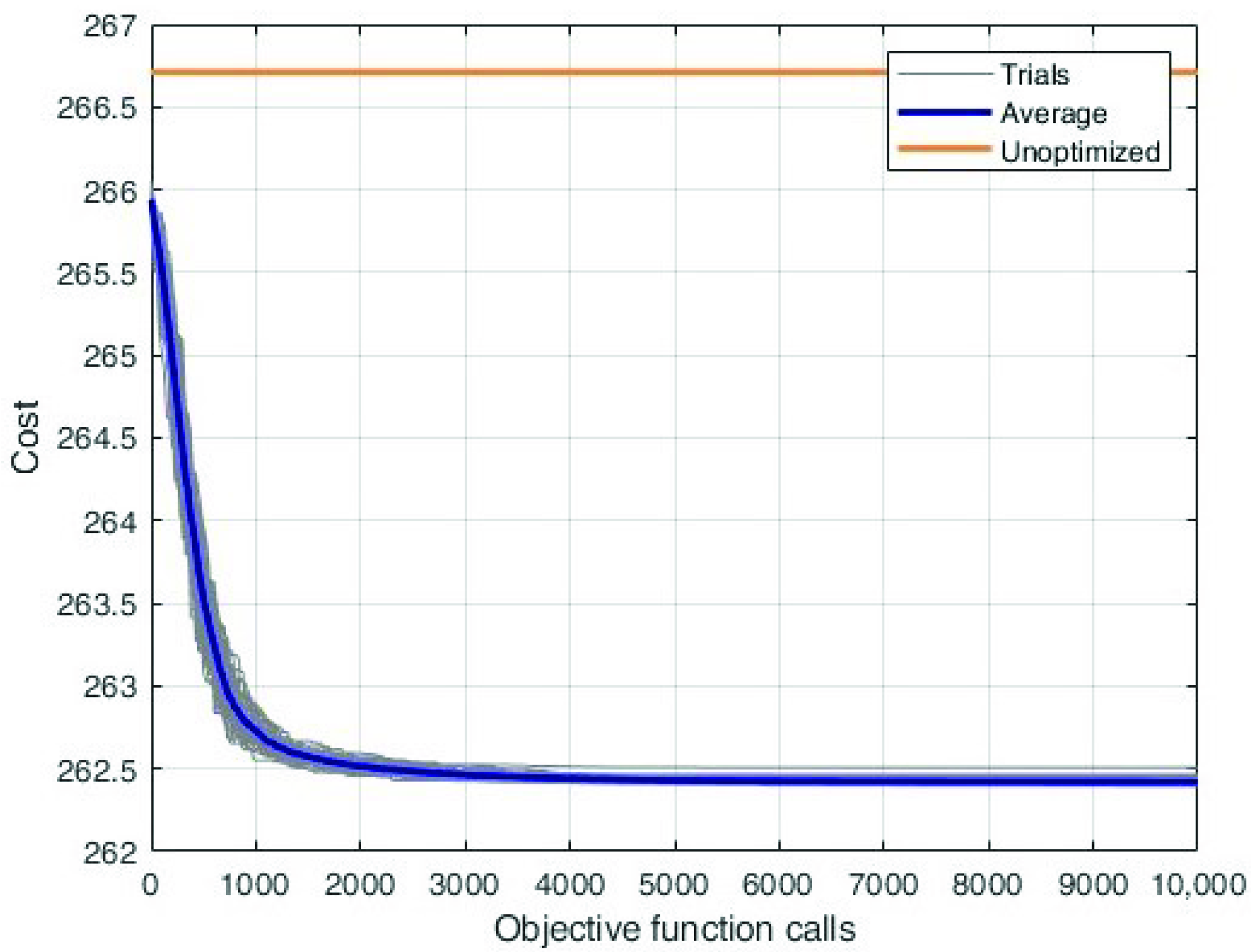
Figure 8 shows the convergence curves for this optimisation: the 50 independent trials are represented by the grey lines; the blue line represent the average convergence and the orange line is the cost value of the unoptimised solution. This last is the load scheduling applied in the company. From these curves, it is possible to notice that all the trials of the algorithm improve with respect to the unoptimised solution. The algorithm convergence is good; however, a deeper analysis will show that it staked in a local minima.
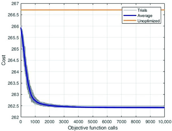
Figure 8.
Convergence curves for the basic optimisation. Each grey line represents one of the 50 independent trials; the blue line is the average convergence; and the orange line is the cost value of the unoptimised solution.
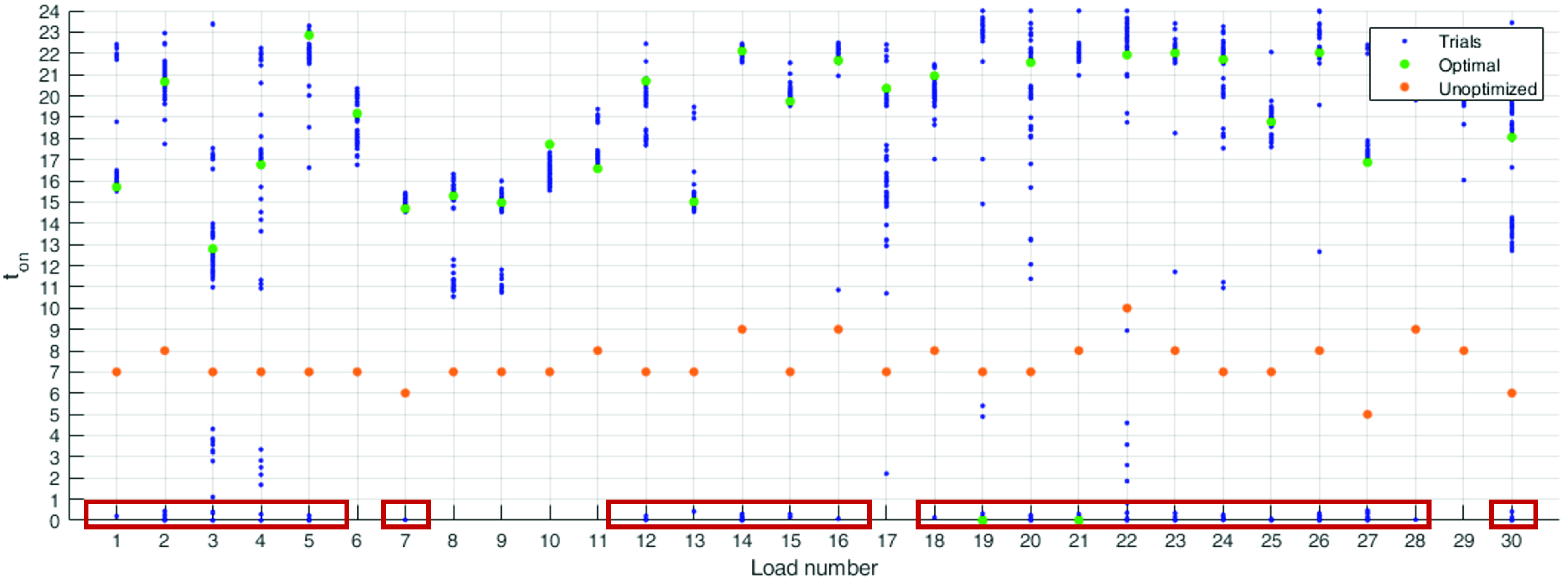
It can be seen in Figure 9 where the optimal solutions of all independent trials are represented: each blue dot represents the value of a final solution in all the 30 design variables. The green dots correspond to the best solution, while the orange ones are the unoptimised design variables. In this figure, it is clear that there are some solutions stacked in the local minima located at the lower boundary of the domain, highlighted by the red squares in the figure.
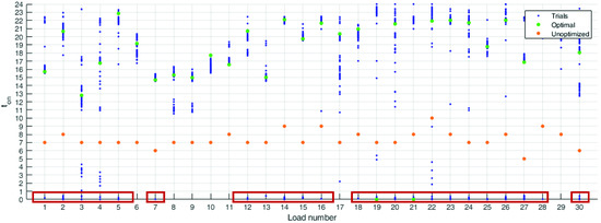
Figure 9.
Representation of the optimal solutions of all the trials: the blue dots represent the value of a final solution in all 30 design variables; the green dots correspond to the best solution; while the orange ones are the unoptimised design variables. The red box highlights the solutions stacked in the local minima.
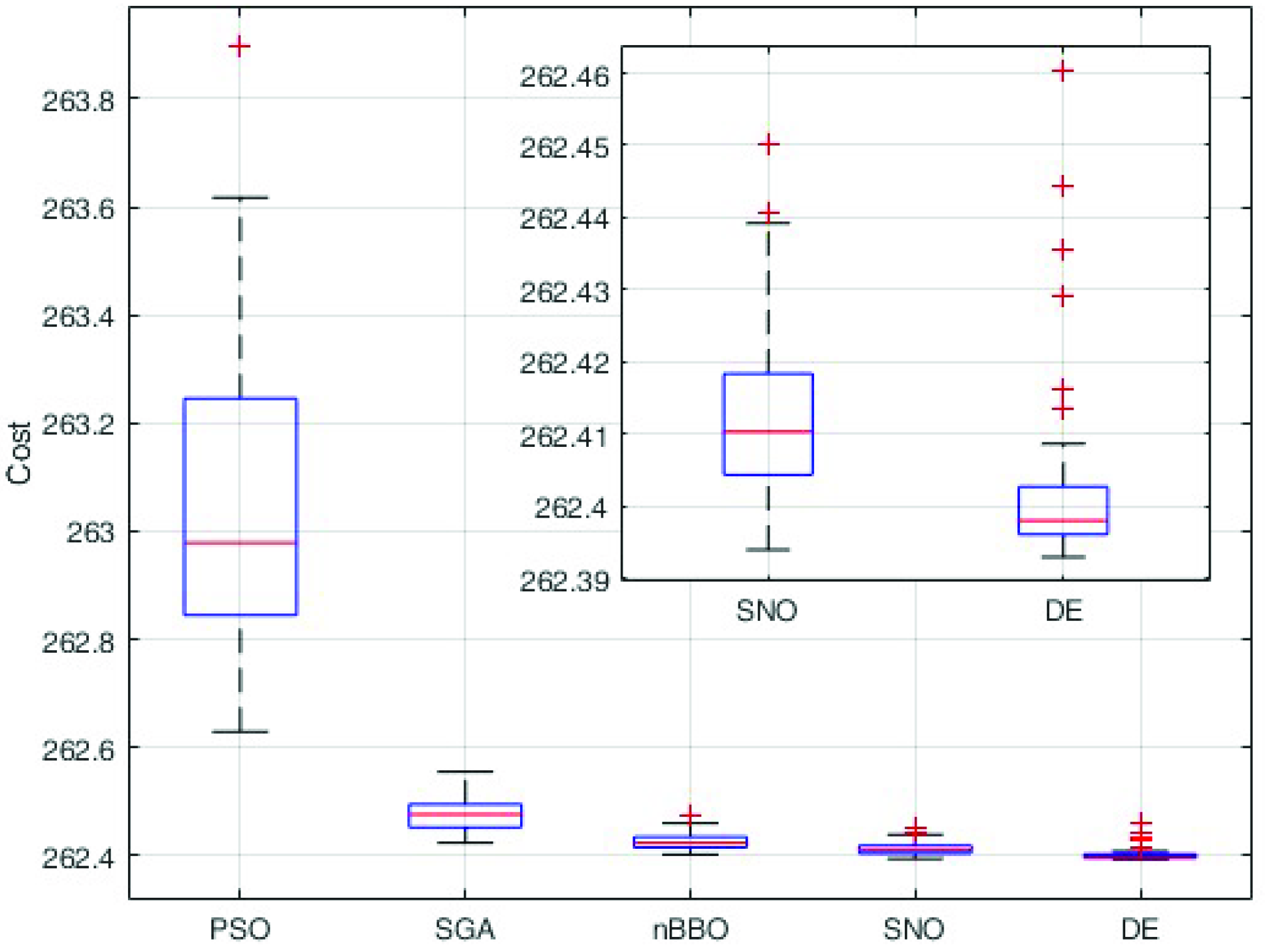
A comparison between different algorithms have been performed in order to justify the selection of the DE for this application. In particular, four other evolutionary algorithms have been tested: the particle swarm optimisation (PSO), the stud-genetic algorithm (SGA), the biogeography-based optimisation (BBO), and the social network optimisation (SNO) [35]. For each algorithm, the termination criterion is set to 10,000 objective function calls; in order to have statistically reliable results, 50 independent optimisation runs were performed. The results of the comparison are shown in the boxplot of Figure 10.
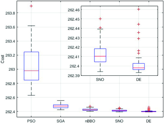
Figure 10.
Boxplot of the comparison between the results obtained by several evolutionary algorithms. The direct comparison between SNO and DE shows that this algorithm is much more reliable.
5.3. Toroidal Correction Optimisation
In order to prevent stagnation on the boundary of the search space, the toroidal correction is introduced in the differential evolution. This is justified from both a theoretical point of view, by the nature of the design variables, and an experimental point of view, by the previously shown results. This optimisation was performed with the same options used beforehand: 50 independent trials and 10,000 objective function calls.
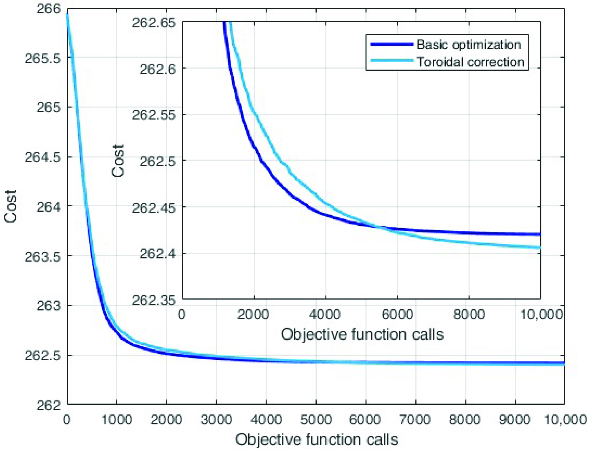
Figure 11 shows the comparison of the average convergence between the base optimisation and the one with toroidal correction. The convergence rate can be seen as the derivative of the convergence curves in Figure 11. The convergence rate is slower for the DE with the toroidal correction, as it can be seen in the zoom in the figure where the light blue line is above the other until 5000 objective function calls. On the other hand, the convergence of the DE with toroidal correction lasts longer, resulting in a lower final cost.
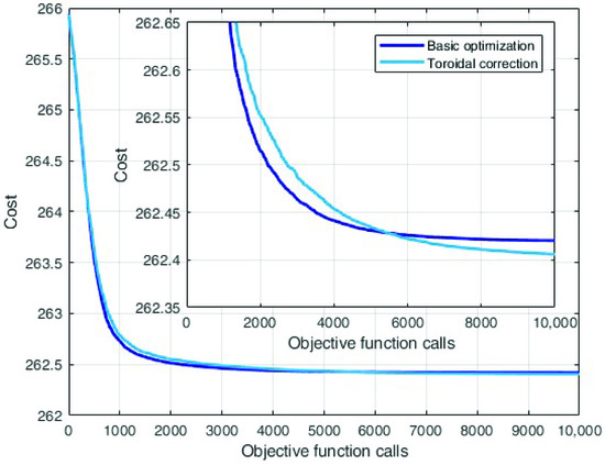
Figure 11.
Comparison between the basic optimisation and the one with toroidal correction.
It is possible to see that the initial convergence is slower, however, it is able to obtain a better final result.
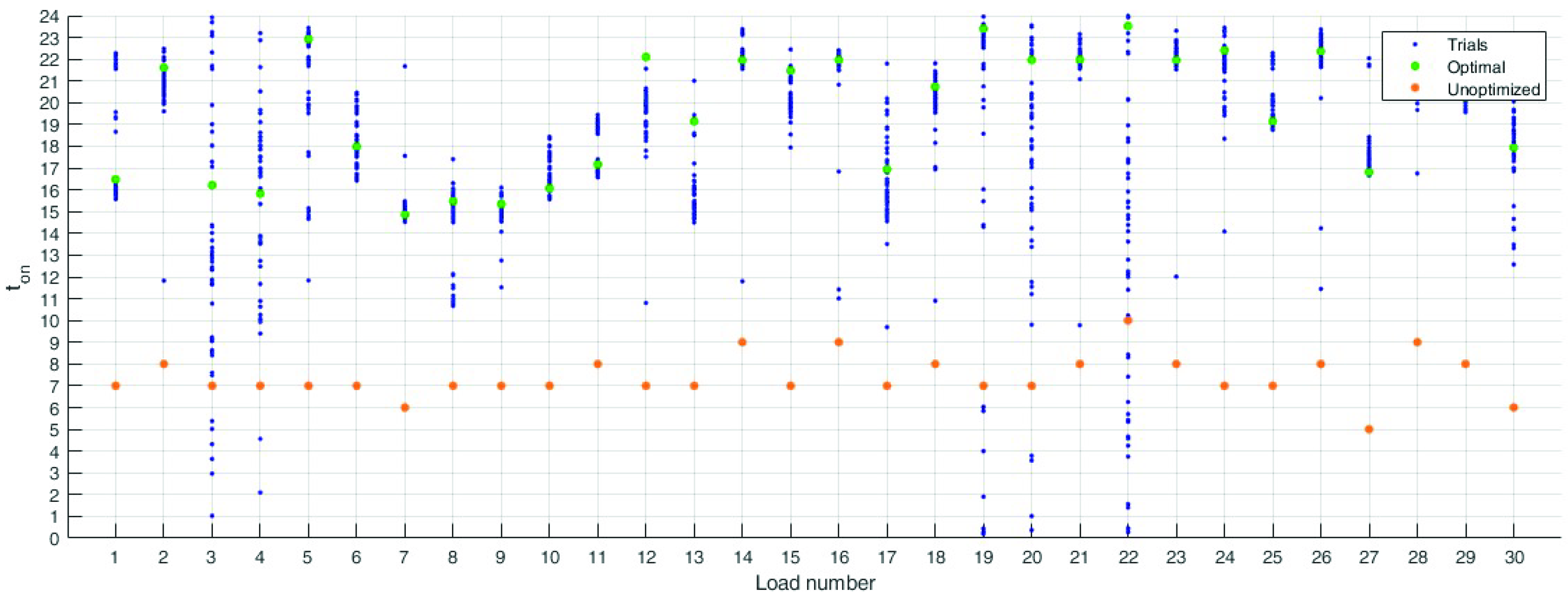
Figure 12 shows that this modification was able to prevent stagnation in the local minima at the lower boundary of the search domain. In fact, the analysis of the values of the optimal solutions shows that there are no solutions stacked at the bottom of the search space. This can be seen by comparing the highlighted part of Figure 9 with the corresponding areas in Figure 12: ultimately, almost no solutions are concentrated in the lower part of the graph.
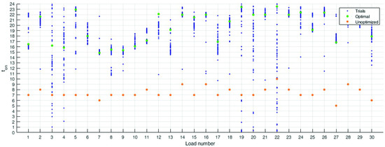
Figure 12.
Distribution of the final solutions with the toroidal correction. The algorithm is able to avoid the local minima on the lower boundary of the search domain.
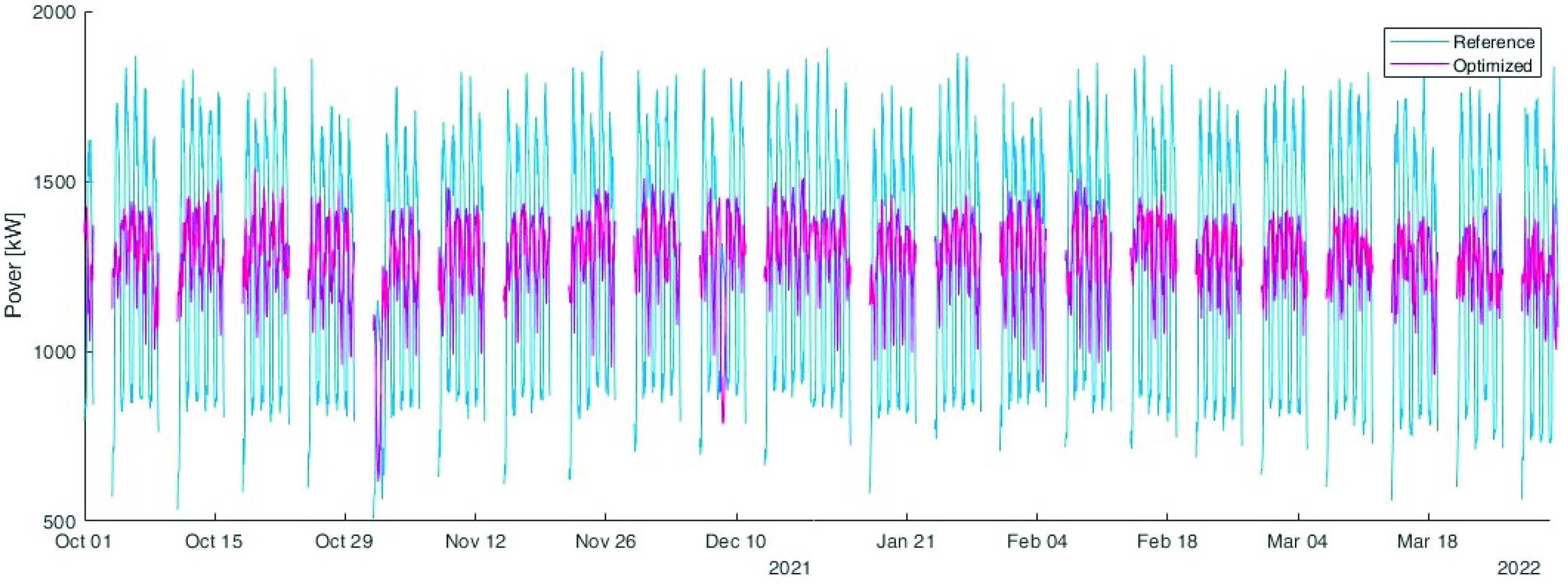
Figure 13 shows the comparison between the reference unoptimised load (in blue) with the optimised one (in purple). This comparison highlights that the peak load was reduced from 1900 kW to 1540 kW.

Figure 13.
Comparison between the reference unoptimised load (in blue) with the optimised one (in purple).
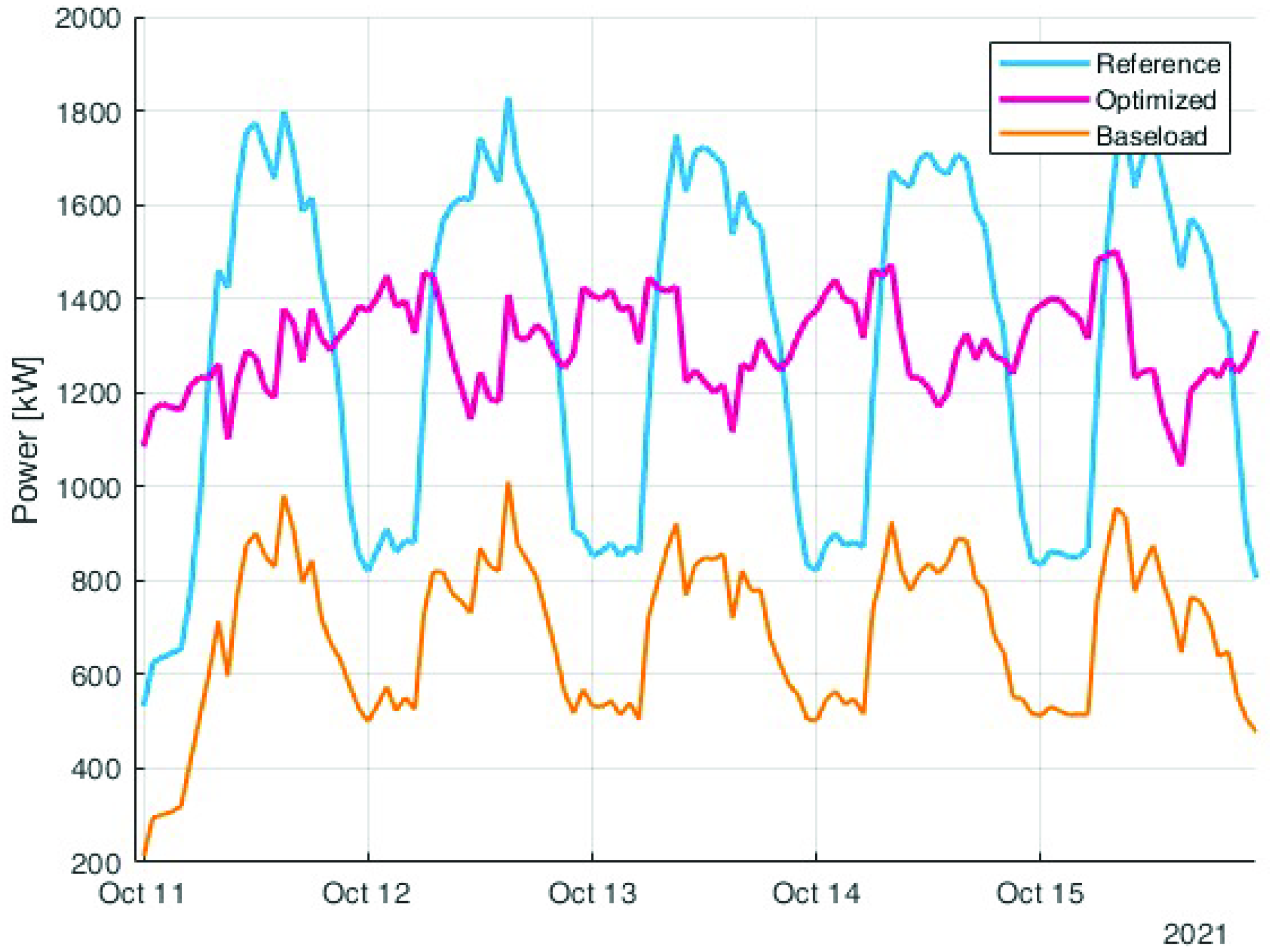
The shift to the night can be better understood by analysing Figure 14 where a sample week is represented. The reference load (in blue) has a very high peak in the hour between 8 a.m. to 8 p.m., while the optimised profile (in purple) is much more constant. The figure also shows the baseload (in orange).
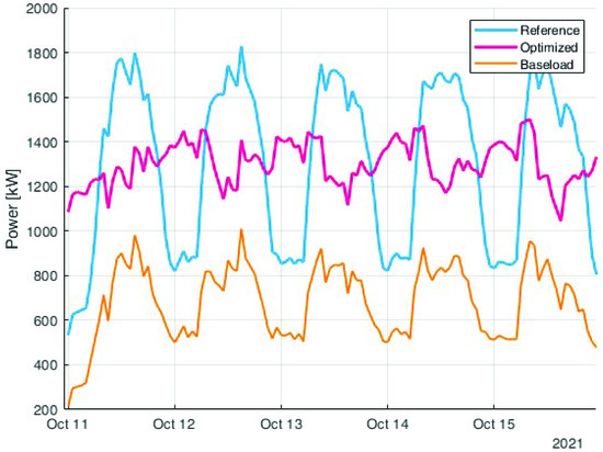
Figure 14.
Zoom of the comparison between the reference load (in blue) and the optimised one (in purple). The orange load is the baseload that cannot be modified by the algorithm.
In this optimisation, the algorithm tends to put the starting times of the loads in the late afternoon/evenings, having loads at night, when the electricity price is lower. Of course, the night shifting of the loads is something undesirable for the company that would prefer daily labour. Constraints can be set to force the optimisation towards daily loads shifting.
In order to make this approach feasible in the real industrial context, the labour cost was introduced as an additional term in the cost function for balancing the optimiser tendency to shift the loads during the night.
5.4. Optimisation with Labour Cost
In order to avoid the problems highlighted in the previous results, the proposed method introduced the labour cost as an additional performance parameter. The optimisation with the labour cost was run 50 times with 10,000 objective function calls. Figure 15 shows the convergence curves of this optimisation.
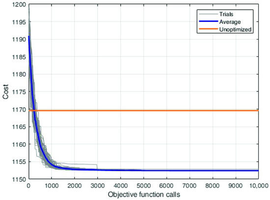
Figure 15.
Convergence curves for the optimisation with labour cost. Each grey line represents one of the 50 independent trials; the blue line is the average convergence; and the orange line is the cost value of the unoptimised solution.
Comparing these curves with those of Figure 8, it is possible to see that the reference solution is better than the algorithm’s random initialisation. The average convergence curve intersects the orange curve, representing the cost of the unoptimised solution, at the beginning of the optimisation process, and then the optimisation process continues to improve. The low dispersion of the solutions demonstrates the robustness of the DE in this framework.
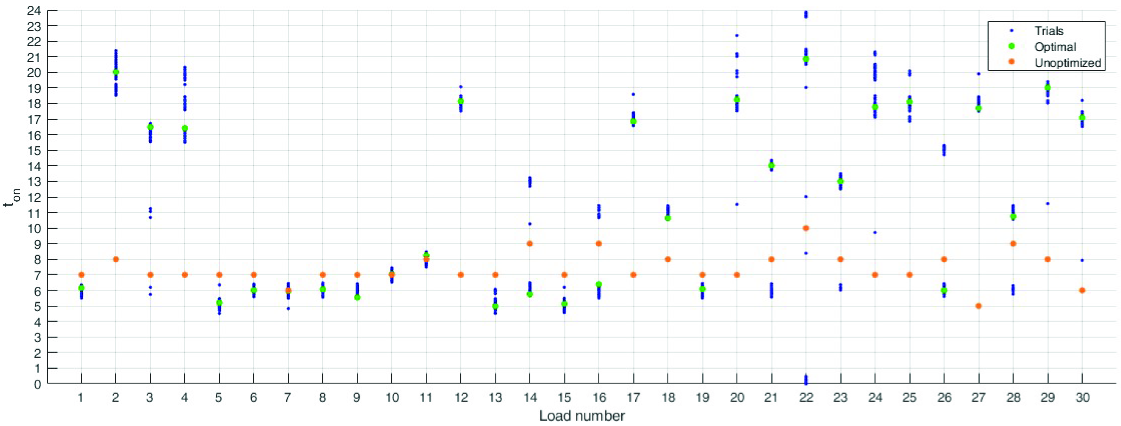
Figure 16 shows the dispersion of the final solutions obtained by the DE, compared with the reference case. This optimisation shows a shift of many loads during the daytime. In particular, 12 loads are located in the night, with a starting time between 5 p.m. and 9 p.m.; 4 loads are shifted in the late morning (between 11 a.m. to 2 p.m.); finally, 14 loads are shifted in the early morning between 6 a.m. to 8 a.m.: these loads exploit the different timing of the electricity tariff and workforce cost.
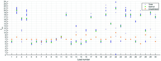
Figure 16.
Distribution of the final solutions with the labour cost. The algorithm shifts several load during the daytime.
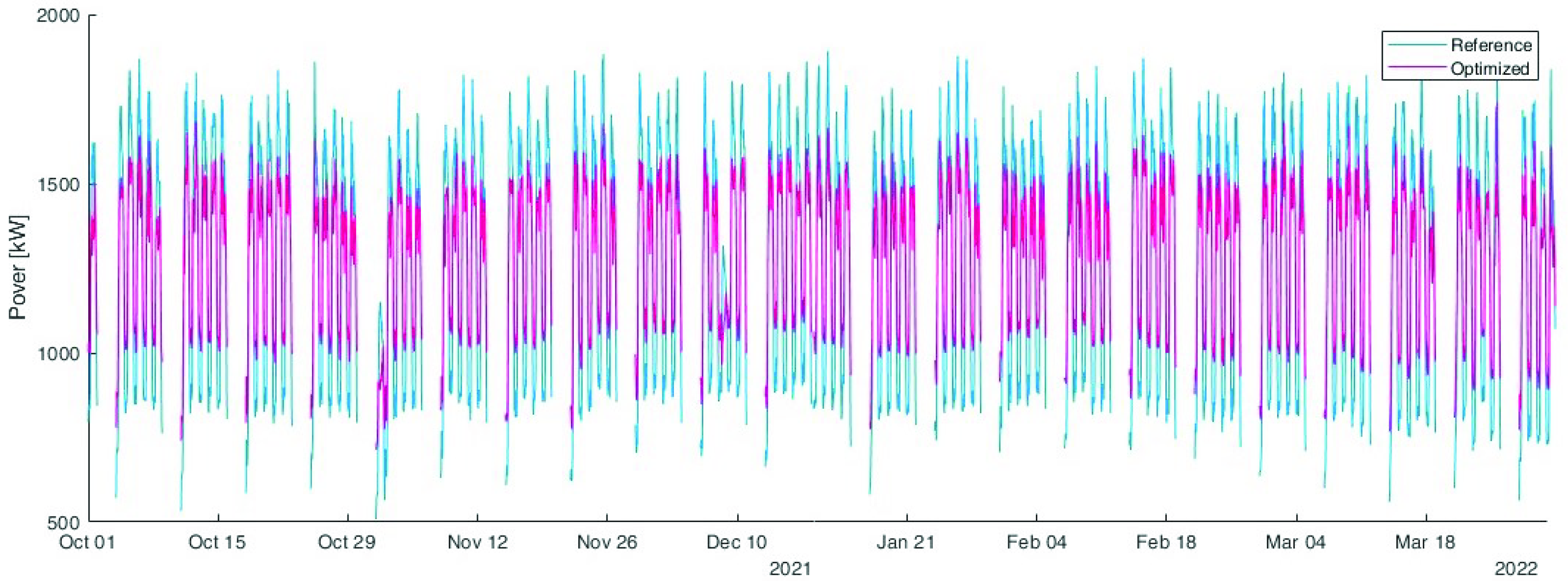
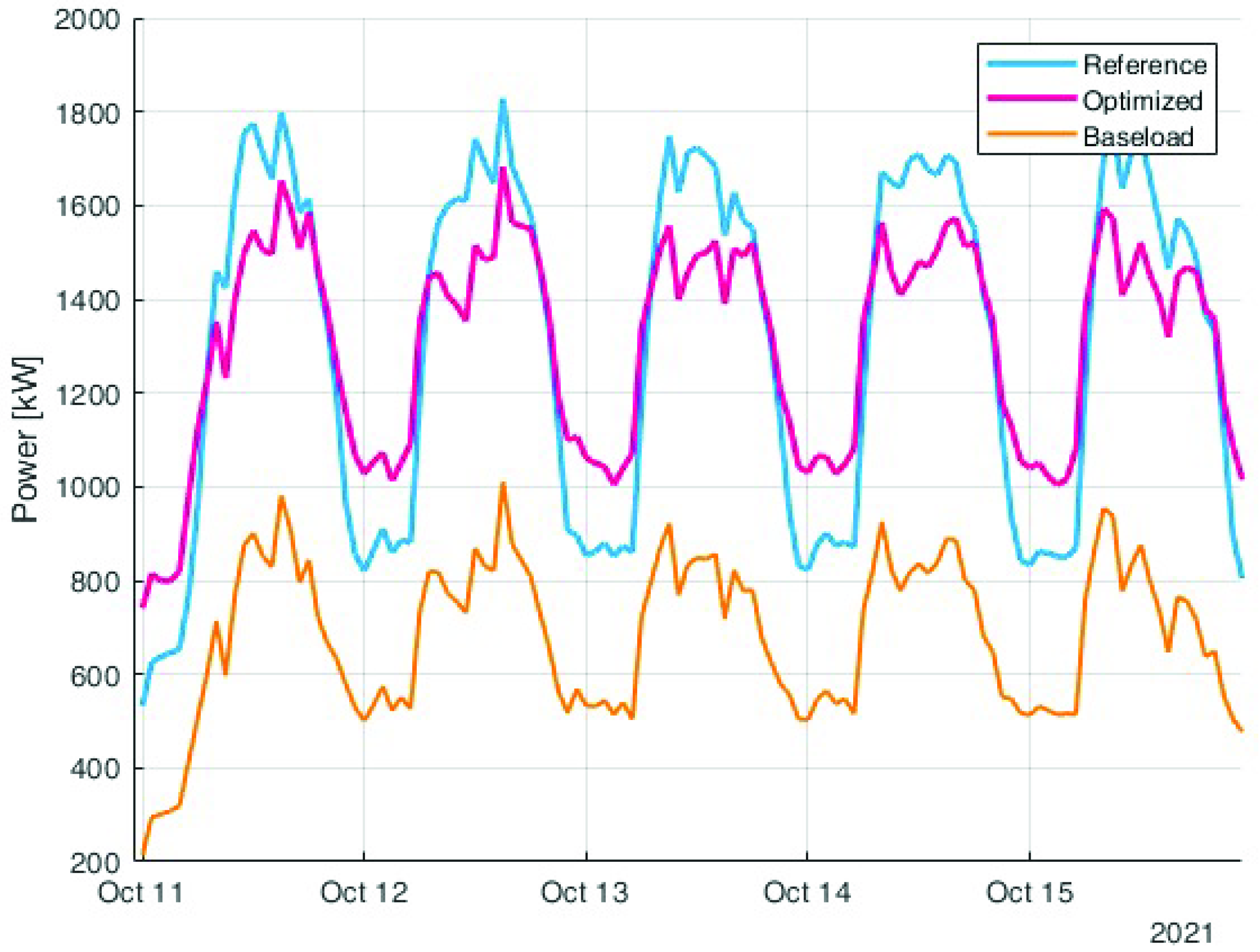
Finally, Figure 17 shows the time profile of the new optimised solution compared with the original one. The peak was slightly reduced from 1900 kW to 1740 kW. The detailed behaviour of the optimised solution compared to the reference one is shown in Figure 18.
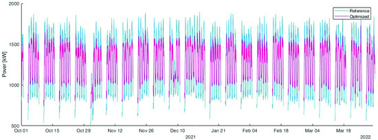
Figure 17.
Comparison between the reference unoptimised load (in blue) with the optimised one considering labour cost (in purple).
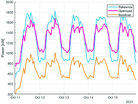
Figure 18.
Comparison over a week between the reference unoptimised load (in blue) with the optimised one considering labour cost (in purple). The orange line represents the baseload that cannot be shifted in the optimisation.
This solution can be implemented in the real industrial context because it produces solutions that find the trade-off between electricity and labour costs.
6. Conclusions
In this work, a demand-side management process based on evolutionary algorithms was designed considering its application in the industrial scenario. For facing the specific issues arisen in this context, two main elements were included in the optimisation process. Firstly, for obtaining an effective convergence and for reducing the algorithm stagnation in a local minima, a toroidal correction was added to the differential evolution. Secondly, two different cost terms were considered for finding an optimal configuration that can be really applied in the industry. These two cost terms are the energy cost and the labour cost.
The cost definition adopted in this work results in a multiobjective problem: in fact, the two cost components are conflicting and arrive at different optimal solutions. In this work, scalarisation was applied considering that both of them are two monetary costs of the company; thus, their sum was minimised.
The proposed system was tested in a real industrial scenario using 6 months of measurements in the analysis (October 2021–March 2022). The optimisation was performed on the 30 loads for which the time profile is available. The final results show a reduction in the total cost from 1169.6 EUR/h of the reference solution to 1152.4 EUR/h, with a reduction of 17.2 EUR/h corresponding to approximately 99,500 EUR/year.
The proposed approach is limited by the small number of loads that can be shifted with respect to the total loads. This can be solved by adding the additional measurements of the power profiles absorbed by the single machines in the industry. The definition of the single machine load profile introduces the need for additional constraints that keep the consistency of the production process where some operations should be run before others.
Author Contributions
Conceptualisation, A.N., G.G.T., F.T., D.M. and E.O.; Data curation, G.G.T.; Formal analysis, A.N., G.G.T., F.T. and D.M.; Funding acquisition, E.O.; Methodology, A.N., G.G.T. and E.O.; Project administration, F.T. and E.O.; Software, G.G.T.; Supervision, A.N., F.T. and D.M.; Validation, A.N. and D.M.; Visualisation, A.N.; Writing—original draft, A.N., G.G.T., F.T., D.M. and E.O.; Writing—review & editing, A.N., G.G.T., F.T., D.M. and E.O. All authors have read and agreed to the published version of the manuscript.
Funding
This research received no external funding.
Data Availability Statement
Restrictions apply to the availability of these data. Data was obtained from Ratti SPA.
Conflicts of Interest
The authors declare no conflict of interest.
References
- Victoria, M.; Zhu, K.; Brown, T.; Andresen, G.B.; Greiner, M. Early decarbonisation of the European energy system pays off. Nat. Commun. 2020, 11, 6223. [Google Scholar] [CrossRef] [PubMed]
- Norouzi, N. Post-COVID-19 and globalization of oil and natural gas trade: Challenges, opportunities, lessons, regulations, and strategies. Int. J. Energy Res. 2021, 45, 14338–14356. [Google Scholar] [CrossRef] [PubMed]
- Wang, M.; Hua, C.; Xu, H. Dynamic Linkages among Carbon, Energy and Financial Markets: Multiplex Recurrence Network Approach. Mathematics 2022, 10, 1829. [Google Scholar] [CrossRef]
- Skjærseth, J.B. Towards a European Green Deal: The evolution of EU climate and energy policy mixes. Int. Environ. Agreem. Politics Law Econ. 2021, 21, 25–41. [Google Scholar] [CrossRef]
- Neagu, B.C.; Ivanov, O.; Grigoras, G.; Gavrilas, M. A new vision on the prosumers energy surplus trading considering smart peer-to-peer contracts. Mathematics 2020, 8, 235. [Google Scholar] [CrossRef]
- Soto, E.A.; Bosman, L.B.; Wollega, E.; Leon-Salas, W.D. Peer-to-peer energy trading: A review of the literature. Appl. Energy 2021, 283, 116268. [Google Scholar] [CrossRef]
- Roberts, M.B.; Bruce, A.; MacGill, I. Impact of shared battery energy storage systems on photovoltaic self-consumption and electricity bills in apartment buildings. Appl. Energy 2019, 245, 78–95. [Google Scholar] [CrossRef]
- Marino, C.; Nucara, A.; Panzera, M.; Pietrafesa, M.; Varano, V. Energetic and economic analysis of a stand alone photovoltaic system with hydrogen storage. Renew. Energy 2019, 142, 316–329. [Google Scholar] [CrossRef]
- Javaid, N.; Hafeez, G.; Iqbal, S.; Alrajeh, N.; Alabed, M.S.; Guizani, M. Energy efficient integration of renewable energy sources in the smart grid for demand side management. IEEE Access 2018, 6, 77077–77096. [Google Scholar] [CrossRef]
- Ivanov, O.; Neagu, B.C.; Grigoras, G.; Scarlatache, F.; Gavrilas, M. A metaheuristic algorithm for flexible energy storage management in residential electricity distribution grids. Mathematics 2021, 9, 2375. [Google Scholar] [CrossRef]
- Jabir, H.J.; Teh, J.; Ishak, D.; Abunima, H. Impacts of demand-side management on electrical power systems: A review. Energies 2018, 11, 1050. [Google Scholar] [CrossRef]
- Kanakadhurga, D.; Prabaharan, N. Demand side management in microgrid: A critical review of key issues and recent trends. Renew. Sustain. Energy Rev. 2022, 156, 111915. [Google Scholar] [CrossRef]
- Cheng, J.; Zhang, G.; Caraffini, F.; Neri, F. Multicriteria adaptive differential evolution for global numerical optimization. Integr.-Comput.-Aided Eng. 2015, 22, 103–107. [Google Scholar] [CrossRef]
- Ahmed, E.M.; Rathinam, R.; Dayalan, S.; Fernandez, G.S.; Ali, Z.M.; Abdel Aleem, S.H.; Omar, A.I. A comprehensive analysis of demand response pricing strategies in a smart grid environment using particle swarm optimization and the strawberry optimization algorithm. Mathematics 2021, 9, 2338. [Google Scholar] [CrossRef]
- Basu, M. Combined heat and power dynamic economic dispatch with demand side management incorporating renewable energy sources and pumped hydro energy storage. IET Gener. Transm. Distrib. 2019, 13, 3771–3781. [Google Scholar] [CrossRef]
- Basu, M. Optimal generation scheduling of hydrothermal system with demand side management considering uncertainty and outage of renewable energy sources. Renew. Energy 2020, 146, 530–542. [Google Scholar] [CrossRef]
- Ivanov, O.; Chattopadhyay, S.; Banerjee, S.; Neagu, B.C.; Grigoras, G.; Gavrilas, M. A Novel Algorithm with Multiple Consumer Demand Response Priorities in Residential Unbalanced LV Electricity Distribution Networks. Mathematics 2020, 8, 1220. [Google Scholar] [CrossRef]
- Parvin, K.; Lipu, M.H.; Hannan, M.; Abdullah, M.A.; Jern, K.P.; Begum, R.; Mansur, M.; Muttaqi, K.M.; Mahlia, T.I.; Dong, Z.Y. Intelligent controllers and optimization algorithms for building energy management towards achieving sustainable development: Challenges and prospects. IEEE Access 2021, 9, 41577–41602. [Google Scholar] [CrossRef]
- Sarker, E.; Halder, P.; Seyedmahmoudian, M.; Jamei, E.; Horan, B.; Mekhilef, S.; Stojcevski, A. Progress on the demand side management in smart grid and optimization approaches. Int. J. Energy Res. 2021, 45, 36–64. [Google Scholar] [CrossRef]
- Wang, Y.; Yang, Z.; Mourshed, M.; Guo, Y.; Niu, Q.; Zhu, X. Demand side management of plug-in electric vehicles and coordinated unit commitment: A novel parallel competitive swarm optimization method. Energy Convers. Manag. 2019, 196, 935–949. [Google Scholar] [CrossRef]
- Xu, F.; Wu, W.; Zhao, F.; Zhou, Y.; Wang, Y.; Wu, R.; Zhang, T.; Wen, Y.; Fan, Y.; Jiang, S. A micro-market module design for university demand-side management using self-crossover genetic algorithms. Appl. Energy 2019, 252, 113456. [Google Scholar] [CrossRef]
- Roy, C.; Das, D.K.; Srivastava, A. Particle swarm optimization based cost optimization for demand side management in smart grid. In Proceedings of the 2019 International Conference on Electrical, Electronics and Computer Engineering (UPCON), Aligarh, India, 8–10 November 2019; pp. 1–6. [Google Scholar]
- Sharma, A.K.; Saxena, A.; Palwalia, D.K. Impact of Divergence in BBO on Efficient Energy Strategy of Demand Side Management. Technol. Econ. Smart Grids Sustain. Energy 2022, 7, 28. [Google Scholar] [CrossRef]
- Sharma, A.K.; Saxena, A. A demand side management control strategy using Whale optimization algorithm. SN Appl. Sci. 2019, 1, 870. [Google Scholar] [CrossRef]
- Soares, A.; Antunes, C.H.; Oliveira, C.; Gomes, A. A multi-objective genetic approach to domestic load scheduling in an energy management system. Energy 2014, 77, 144–152. [Google Scholar] [CrossRef]
- Soares, A.; Melo, H.; Antunes, C.H.; Trovao, J.P.; Gomes, A.; Jorge, H. Integration of the electric vehicle as a manageable load in a residential energy management system. In Proceedings of the 2015 IEEE Vehicle Power and Propulsion Conference (VPPC), Montreal, QC, Canada, 19–22 October 2015; pp. 1–6. [Google Scholar]
- Antunes, C.H.; Soares, A.; Gomes, Á. An energy management system for residential demand response based on multiobjective optimization. In Proceedings of the 2016 IEEE Smart Energy Grid Engineering (SEGE), Oshawa, ON, Canada, 21–24 August 2016; pp. 90–94. [Google Scholar]
- Soares, A.; Gomes, Á.; Antunes, C.H.; Oliveira, C. A customized evolutionary algorithm for multiobjective management of residential energy resources. IEEE Trans. Ind. Inform. 2016, 13, 492–501. [Google Scholar] [CrossRef]
- Ogunjuyigbe, A.; Ayodele, T.; Akinola, O. User satisfaction-induced demand side load management in residential buildings with user budget constraint. Appl. Energy 2017, 187, 352–366. [Google Scholar] [CrossRef]
- Favre, L.; Robyr, J.L.; Gonon, F.; Niederh, E.L. Improvement of the environmental impact of the global energy management of buildings by genetic algorithm optimization. In Proceedings of the 2018 5th International Conference on Electric Power and Energy Conversion Systems (EPECS), Kitakyushu, Japan, 23–25 April 2018; pp. 1–6. [Google Scholar]
- Pretto, S.; Ogliari, E.; Niccolai, A.; Nespoli, A. A New Probabilistic Ensemble Method for an Enhanced Day-Ahead PV Power Forecast. IEEE J. Photovoltaics 2022, 12, 581–588. [Google Scholar] [CrossRef]
- Storn, R.; Price, K. Differential evolution—A simple and efficient heuristic for global optimization over continuous spaces. J. Glob. Optim. 1997, 11, 341–359. [Google Scholar] [CrossRef]
- Caraffini, F.; Kononova, A.V.; Corne, D. Infeasibility and structural bias in differential evolution. Inf. Sci. 2019, 496, 161–179. [Google Scholar] [CrossRef]
- Kononova, A.V.; Caraffini, F.; Bäck, T. Differential evolution outside the box. Inf. Sci. 2021, 581, 587–604. [Google Scholar] [CrossRef]
- Grimaccia, F.; Mussetta, M.; Niccolai, A.; Zich, R.E. Comparison of binary evolutionary algorithms for optimization of thinned array antennas. In Proceedings of the 2018 IEEE Congress on Evolutionary Computation (CEC), Rio de Janeiro, Brazil, 8–13 July 2018; pp. 1–8. [Google Scholar]
Publisher’s Note: MDPI stays neutral with regard to jurisdictional claims in published maps and institutional affiliations. |
© 2022 by the authors. Licensee MDPI, Basel, Switzerland. This article is an open access article distributed under the terms and conditions of the Creative Commons Attribution (CC BY) license (https://creativecommons.org/licenses/by/4.0/).


