Abstract
Model-based controllers suffer from the effects of modeling imprecisions. The analytical form of the available model often contains only approximate parameters and can be physically incomplete. The consequences of these effects can be compensated by adaptive techniques and by the improvement of the available model. Lyapunov function-based classic methods, which assume exact analytical model forms, guarantee asymptotic stability by cautious and slow parameter tuning. Fixed point iteration-based adaptive controllers can work without the exact model form but immediately yield precise trajectory tracking. They neither identify nor improve the parameters of the available model. However, any amendment of the model can improve the controller’s operation by affecting its range and speed of convergence. It is shown that even very primitive, fast, and simple versions of evolutionary computation-based methods can produce considerable improvement in their operation. Particle swarm optimization (PSO) is an attractive, efficient, and simple tool for model improvement. In this paper, a PSO-based model approximation technique was investigated for use in the control of a three degrees of freedom PUMA-type robot arm via numerical simulations. A fixed point iteration (FPI)-based adaptive controller was used for tracking a nominal trajectory while the PSO attempted to refine the model. It was found that the refined model still had few errors, the effects of which could not be completely neglected in the model-based control. The best practical solution seems to be the application of the same adaptive control with the use of the more precise, PSO-improved model. Apart from a preliminary study, the first attempt to combine PSO with FPI is presented here.
MSC:
37M10
1. Introduction
The difficulties in creating satisfactorily precise dynamic models of robots in a direct (i.e., not control task-related) manner have been well explored in the 1990s [1]. For modeling other physical systems, such as turbo jet engines, tremendous efforts must be made from the “diagnostics side” (e.g., through observing the magnetic field around the engine [2], or the application of thermal imaging diagnostics methods [3]). A quite complicated numerical design methodology must be applied to improve the operation of turbo jets by injecting water into the system: in this case, the generated steam serves as the working medium of the classical steam engines (e.g., [4]). However, these very complex investigations normally result in a relatively simple and primitive “dynamic model” that can be utilized for control purposes (e.g., [5,6]). These “simplified models” are only approximations of reality. This fact emphasizes the significance of the use of the adaptive techniques that cannot be completely evaded by the application of “precise models”. In general, both the improvement of the available model, i.e., the application of sophisticated adaptive techniques as well as the combination of these approaches, may be possible ways for improving the operation of the controlled system. In the sequel, both possibilities are briefly considered.
1.1. On the Adaptive Control Techniques
The adaptive controllers can be classified into two major groups based on the available information on the dynamic model of the controlled system. In the first group, the analytical form of the dynamic model is available, and only the parameters of this model are approximately known. In this case, the adaptation can be regarded as parameter identification online. The classic prototypes of this method are the adaptive inverse dynamics controller and the Slotine–Li adaptive controller for robots from the 1990s [7]. This approach is based on Lyapunov’s Ph.D. dissertation from 1892 [8,9], which became the mathematical foundation of the prevailing control design methods used even in our days (e.g., [10,11,12]).
In the other group, the appropriate feedback signal is applied on the basis of the actual observations without the need for “learning” or elaborating on an “exact model”. The prototype of this signal adaptation-based technique is the model reference adaptive controller (MRAC) from the 1990s [13]. This controller, in addition to guaranteeing precise trajectory tracking, has the additional function of making the observable behavior of the controlled system similar to that of a stable linear system for an external control loop by the application of fast feedback signals. In this case, the external control loop can apply linear system–tailored design methods. This approach also uses the Lyapunov function-based technique in the design. A typical alternative example of this approach is the fixed point iteration (FPI)-based adaptive control using Banach’s fixed point theorem from 1922 [14]. Its prototype was suggested in 2009 in [15]. The main aim was to evade the use of the complicated Lyapunov function-based design and replace it with a simpler method. The essence of the method is that it determines a trajectory tracking strategy on the basis of purely kinematic considerations, and adaptively deforms the “desired time derivative of the system’s generalized coordinate” before utilizing it in the available approximate dynamic model for the calculation of the necessary control force. It was successfully applied in the development of a novel type MRAC controller [16]. Later, several variants were elaborated on and their applicability was investigated via simulations in various tasks, such as the control-based treatment of patients suffering from type 1 diabetes [17], and in the adaptive version of the receding horizon controller in [18]. The first experimental verification of the method was done in the adaptive control of a small electric motor in a BSc thesis in 2018 [19]. In this solution, simple Arduino components were used without the application of any noise filtering technique. For less ideal systems burdened by huge measurement noises, dead time, and delays, preliminary investigations were made for the classical computed torque controller [20]: the controlled system was a propeller-driven pendulum with considerable friction in its bearing in [21]. Since then, not yet published experimental results have been collected for the FPI-based adaptive control of this system. In general, with regard to the noise effects, it can be stated that for keeping some “static position” of the controlled system without noise filtering, the non-adaptive version is always better than the adaptive one in the control of this second-order system, because the second time derivatives fed back are noise-burdened; in this case, the noise/signal ratio is . However, in the strongly dynamical part of the motion in which the essential second time derivatives of the signal are significant, this ratio becomes much better and the adaptive control has benefits. Applications of simple and efficient noise filtering techniques (e.g., as used in [22]) can make this problem insignificant. This expectation is also supported by the existence and success of acceleration feedback controllers (e.g., [23,24,25]).
Though this approach does not invest any effort in amending its originally given approximate analytical model, it does not exclude the possibility of simultaneously improving this model. In [26], the original error feedback term of the classic adaptive inverse dynamics controller (AIDC) was so modified that the FPI-based approach guaranteed precise trajectory tracking even at the beginning of the control session (when the dynamic model applied was imprecise). Since this feedback term made it possible, the operation of the Lyapunov function-based parameter tuning of the AIDC, following a slow and cautious tuning process the model, became very precise, and the FPI-based signal deformation became quite insignificant at the end. A similar modification of the other classic approach, the Slotine–Li adaptive controller, was published in [27]. This controller is also based on Lyapunov’s tuning technique but it uses a Lyapunov function that is different from that of the AIDC controller. All of these approaches have the common feature that they dynamically couple the trajectory control process with parameter tuning.
Following the above examples, the idea naturally arose whether it was possible to combine the FPI-based adaptive controller with other learning methodologies to improve the available dynamic model. The present paper concentrates on this issue.
1.2. Improvement of the Dynamic Model by the Use of Evolutionary Methods
In general, parameter identification or other model improvement methods can be formulated as optimization tasks in which some cost terms constructed of error-type components have to be minimized. For dealing with differentiable cost functions, the oldest method is Lagrange’s “Reduced Gradient Method”; he originally developed it for the analytical formulation of the principles of classical mechanics in 1811 [28]. It allowed restricting the optimum search over some smooth, differentiable, hypersurfaces embedded in the search space via Lagrange multipliers. Lagrange’s method has become the prototype of mathematical formulations in modern theoretical physics. For instance, finding the appropriate Lagrangian for describing dissipative phenomena has been an active research area in recent years [29,30]. Based on the analogies with classical mechanics, it has also become the main paradigm of optimal controllers using dynamic programming [31,32].
To resolve the restrictions originating from the use of differentiable cost functions, the simplex method was proposed in 1965 [33,34]. Its convergence properties were the subjects of scientific analyses, even in recent years (e.g., [35]). In the simulated annealing approach, the gradient descent method was combined with stochastic components in the 1980s (e.g., [36]).
By dropping the restriction of differentiable cost functions, new perspectives opened up for the use of bio- and martial arts-inspired heuristic solutions, such as genetic algorithms [37] that are actively used for optimization in our days (e.g., [38]). In the memetic algorithms, the results of the evolutionary methods are refined in the final steps via gradient-based methods (e.g., [39,40,41]). It is almost impossible to count the large number of witty algorithms that have been inspired by the behaviors of animals. Perhaps the latest includes the starling murmuration-based optimization [42], moth–flame optimization [43,44], and the quantum-based avian navigation-based optimizer algorithm inspired by the extraordinary precision of the navigation of migratory birds during long-distance aerial paths [45], which is an improvement of the original idea formulated in [46].
The particle swarm optimization (PSO) is one of the first socialization algorithms that mimic the social behaviors of the population and the interactions between individuals—a so-called swarm-based approach. The first example of PSO was published in 1995 when Kennedy and Eberhart developed mathematical and coding concepts [47]. Its flexible ability to tackle and solve many difficult problems has been approved, and it is used as a powerful optimization tool in many applications, e.g., solving temporospatial boundary condition problems [48], efficient smart city planning, heating load estimations [49,50], energy consumption [51], cloud computing [52], and Internet of things applications [53,54].
The PSO—in addition to its fast convergence, stable response, and usage in a wide range of problems of different natures—can easily be implemented and combined with other mathematical techniques. Since the method can learn, it can be directed toward the suitable task goal and, thus, it has become an attractive research area. It can absorb modifications and improvements. There are many proposals for improving PSO due to the complexity of the problem. In [55], leaving and researching mechanisms were introduced to the PSO algorithm. In [56], an adaptive weighted delay velocity (PSO-AWDV) was introduced. Additionally, the PSO is used to maintain the parameters in which benefits from the power of coupled algorithms are expected, as in [57], where PSO was used in cooperation with an artificial neuro-fuzzy inference system (ANFIS), and with the sliding mode control (SMC) to obtain sliding surface parameters to control the robot manipulator. In [58], the authors utilized it to optimize the input feature of the ELM (extreme learning machine) network when proposing a classification of any input feature variation from the optimal value. The fast operation of PSO can be used to find a global solution in combination with a local search method based on Lyapunov’s theory [59].
For the evaluation of evolutionary algorithms in practice, various test systems can be used. Since PSO is well applicable for non-convex optimization tasks, its success strongly depends on the nature of the cost function to be optimized. Perhaps the most rigorous test function is the Rastrigin probe, i.e., an everywhere continuous and differentiable function (in two dimensions). It has an absolute minimum, but this minimum is surrounded by plenty of local minima that provide only a little bit of a higher value than the absolute minimum. The idea was published in 1974 [60] and it soon was applied for test purposes in optimization [61]. The density of the local minima can be manipulated via scaling the coordinates of this function. Evidently, for the PSO algorithm, it is not important to approach the global optimum by each particle, by increasing the density of the particles in the search space, and manipulating the speed of the random motion; thus, the odds of well approximating the global optimum can be increased. It can be assumed that Rastrigin’s idea was motivated by the famous example by Weierstraß in 1872 [62]. He proved (by his constructive proof) that there exists everywhere continuous (but nowhere differentiable) functions. Finding the global optima of such functions could serve as an ultimate challenge for evolutionary methods. Evidently, in practical applications, the appropriate scaling can be known or at least guessed in advance. While in many applications, the quality of the applied random number generator has considerable significance, especially in the inverse problem theory where Monte Carlo integration is applied (e.g., [63]), or in the case of designing novel versions of Kalman filters (e.g., [64,65,66]); this issue is less important in the most primitive forms of the classic PSO algorithms. To drive the particles toward a given direction, a simple random number generator working in the domain can work well. To kick out the particles of a local minimum, a similar one working in the interval can work well. For such purposes, a simple even distribution over the interval can be satisfactory. The Kalman filters normally assume Gaussian distribution.
1.3. Preliminary Conclusions for the van der Pol Oscillator
To improve the model used by the FPI-based adaptive controller, our first choice in this direction was the PSO-based approach (due to its simplicity and ingenious nature). In [67], only a very primitive, small-dimensional problem was investigated in the control of a mechanical device containing coupled parasite dynamical components. Complicated Lie derivatives of a model were substituted by a simple affine term of constant coefficients. For more precise parameter identification in [68], preliminary investigations were made concerning the application of this idea with the adaptive control of a typical strongly nonlinear benchmark system—the van der Pol oscillator [69]. To apply fast real-time solution, it was assumed that it would be satisfactory to consider only the “recent lump” as a smaller part of the already visited dynamic state space for the evaluation of the fitness of the particles. However, it was found that in this manner no convincingly convergent behavior of the PSO was observed. It was also found that the success of the parameter identification strongly depended on the nominal trajectory that had to be tracked by the controller.
To explain this situation, it is expedient to consider the geometric interpretation of the parameter identification process based on the dynamic model of the controlled system. In the case of the van der Pol oscillator, the model is given in (1)
in which q denotes the generalized coordinate of the system, and u is the control force. The dimension of the parameter space is 4, i.e., the independent parameters can be arranged in an array as . In principle, if one makes 4 independent measurements for the associated quantities , 4 independent equations of the common form in (1) can be obtained. These equations may have unique solutions. However, the equations can be so chosen that they have to provide satisfactory information on each system parameter. For instance, if only the free motion of the system is measured with , then the term will not give enough information on m. If in the observed set utilized by the PSO algorithm u is underrepresented, neither m nor the other parameters can be found by a convergent algorithm. In a similar manner, if only small values are present in the measured set, parameter k will be underrepresented. Moreover, if the values are in the close vicinity of a, it is hopeless to identify parameter b. Furthermore, if only small values are considered, neither parameter a, nor parameter b can be well identified. Therefore, the set of the measured values needs to be redundant and well balanced to obtain satisfactory results for the parameter identification.
Evidently, similar questions may arise in the case of different system models. In each case, the structure of the system’s model determines the practical meaning of the “well balanced set”. Consequently, in the case of the robot parameter identification task, the dynamic model of the robot has to be investigated. In general, it has the form
in which the positive definite symmetric matrix , and the array contain the model parameters, is the generalized control force that has to be exerted by the robot’s drives, and is the array of the generalized coordinates of the robot.
Regarding the qualitative description of the model, it may occur that, at certain points, is ill-conditioned (though it cannot be exactly singular). In these points, certain components play non-significant roles in the identification. Moreover, it is known that the term is quadratic in the components of ; therefore, for good parameter identification, it is expedient to consider high components. Without considering other particular analytical details of the dependence of and on the independent parameters of the identification task, no more statements can be done. The detailed model given in (6)–(8) has a complicated structure; therefore, it does not make sense to go into a detailed analysis of the parameter sensitivity in the identification task.
On this basis, it can be expected that in the case of the model in (2) for the evaluation of the particles, their behaviors in the formerly visited and observed state space would be necessary or at least expedient. This means that as time passes by, the space for the evaluation of the particles can drastically increase. However, for practical reasons, the size of this set must be limited.
The structure in (6)–(8) anticipates that if the model altogether has independent parameters, (2) may support satisfactory information on the model parameters if we have only the same number, i.e., K independent observations. In an appropriate number of combinations of the values q, , , and Q, these few examples would convey satisfactory information for finding the parameters. This observation allows one to believe that a very huge observed state space lump is not necessary to solve this problem. A set that is a little bit larger may contain certain redundancies that must not generate problems in the solution.
In the sequel, at first, the essence of the fixed point iteration-based adaptation is briefly explained in Section 2. The details of the dynamic model of the robot arm considered are given in Section 3. In Section 4 the PSO algorithm is briefed. The simulation results are provided in Section 5, and in Section 6 their discussion is given. Finally, the conclusions of the research are given in Section 7.
2. The Adaptation Strategy in the FPI-Based Control
The “fixed point iteration-based (FPI) adaptive controller” is considered a further developed version of the “Computed Torque Control” [20] method that uses the “Exact Model” to evaluate the control signal for the controlled robot. If the model is not precise (either in its parameters or even in its structure), the required kinematic data (e.g., in the case of a second-order system, the desired second time derivatives of the generalized coordinates) are adaptively deformed before being introduced into the available imprecise model. The appropriate deformation is found when the realized second time derivative will be equal to the desired one. In this case, the kinematically (kinetically) designed trajectory tracking policy is realized and precise tracking control can be achieved. From a mathematical point of view, the appropriate deformation is found via iteration. The control task is mathematically transformed SO that the solution is a fixed point of a contractive map to which, according to Banach’s theorem, the iteration converges. From A technical point of view, in a digital realization of the control, during one control cycle, only one step of the adaptive iteration can be realized. However, if the kinematic design is based on feeding back only the PID-like terms of the tracking error, and the controller is able to abruptly modify the second time derivatives, the method can work in a practically satisfactory manner. the fixed point to be tracked by the adaptive controller slowly varies in time, according to the properties of the nominal trajectory and the PID-type feedback. It works according to the following steps which are represented by the flowchart in Figure 1:
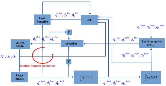
Figure 1.
The PSO’s operation flow chart. The PSO block takes the information from the realized coordinates , their first time derivatives , and the control torque components so that it can calculate their estimated second time derivatives . These estimated values will be evaluated and compared with the realized second derivatives via the cost function defined as . Here, the usual process of PSO handles to search journey toward the global minimum in respect of the defined particles that can be found in Section 4. The dynamics of the PSO-based parameter tuning is not coupled to that of the adaptive control, in contrast to the operation of the classic tuning methods. The iterative sequence of the FPI-based adaptive controller is formed within the loop as indicated in the chart by a red curve.
- The “Kinematic Design” where the “Desired Signal” is generated, based on a PID-type design using the difference between the nominal coordinate and the real one as an error , the integrated error as , and the derivative of the error . In our approach, the controller is used with defining a single constant parameter unlike the common PID gains, which are independent parameters, such as , and , and normally they require continuous tuning. In our case, as it is given in (3), the special gains correspond to , , and :
- The “Adaptive Deformation Signal” generated by deformation of the desired second derivative . Various mathematical deformations can be applied. Since the studied system is a multi-degree-of-freedom system, the adaptive deformation in this paper applied the “Abstract Rotation-based Fixed Point Transformation” published in [70], which realizes Algorithm 1.
- In the “Approximate System Model”, the control force is computed based on the adaptively deformed signal. This force will be applied to the controlled system (“Actual System”) so that the realized second derivative coordinate is obtained.
The sequence of the adaptively deformed signals consists of the elements in which , as can be seen in the feedback loop in Figure 1, which also conveys information on the parameter identification process that is explained in Section 4.
The essence of Algorithm 1 intuitively can be highlighted in the symbolic picture in Figure 2
| Algorithm 1 The abstract rotation-based fixed point transformation algorithm |
| Require: |
| Ensure: |
| ▹ Rodrigues formula |
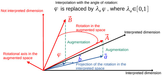
Figure 2.
The symbolic description of the “abstract rotations”: the vectors of physically interpreted components are so augmented into the vectors by adding further orthogonal components to them that in the sense of the Frobenius norm. These vectors determine a TWO-dimensional plain within which B can be rotated into A with angle . The axis of the rotation is the -dimensional orthogonal subspace of this plain. Due to this rotation the physically interpreted projection of B, which is b, is exactly transformed into the physically interpreted projection of A, i.e., into a. The projections suffer rotation and dilatation or shrinking in . With the parameter , by making a rotation only with the angle instead of some nonlinear interpolation can be realized.
With regard to the possible convergence of the adaptation process (2) can be considered. If and are the approximate model components, and and denote the exact ones, by the use of the deformed signal the realized can be computed as follows:
In [70], as the generalization of the concept of the single variable monotonic increasing function for multiple variable cases, the approximately direction keeping function was defined in the following manner: if the value , then is approximately direction keeping. Evidently, if someone wishes to achieve some “desired” , in the case of such a function, he/she can iteratively find an appropriate input . A car driver, who is an intelligent adaptive system, can learn driving a particular car if the steering wheel, the accelerator, and the brake pedals behave appropriately. In a similar manner, a fixed point iteration can be made convergent for such systems. If in (4b) the deformation is realized by the linear operator D as , it is concluded that
that can be made approximately direction keeping by choosing with leading to . That is, many appropriate adaptive deformations exist, and the fixed point iteration can find a solution to the problem. More sophisticated and more general considerations for convergence can be found in [71].
3. Model Dynamics
The simulations were made in Julia language with time resolution s by using the 3-DOF robot system that can be realized by Equations (6)–(8) in which the following shortcuts were applied for simplifying the appearance as possible: , , , , , .
Table 1 contains the parameters of the exact model to realize the original system behavior and the approximate model parameters used by the adaptive controller.
4. Implementation of the PSO Strategy
For estimation of the robot model, five parameters () were chosen: , , , , and . These parameters were placed in a row as input. For the effective minimum value search, the sixth place was reserved for the cost function, which was computed by the absolute value of the difference between the estimated and the realized (observed) values.
For initializing the PSO particles, a non-empty grid of points was set (i.e., it consisted of a set of random populations with Initial Values ) so that the evaluated particles could move accordingly. The number of particles was set to 32.
The velocity of the ith particle had the following form, which was a bit amended based on the “Simulated Annealing” method [36] by adding a complementary random term to the original ones. In the simulated annealing method, the role of this term involved kicking out the solution from a small local optimum. The equation of motion of the particles is given in (9).
The function in (9) corresponds to an even distribution between While in the “traditional terms” the particle is “pulled toward” the local or global optima, the last term can have an arbitrary direction weighted by the parameter .
The flowchart in Figure 1 explains the signals directly fed from FPI-based control , and Q that are used to calculate the estimated acceleration for each robot link as . These estimated values are compared to the real second coordinate time derivatives that are obtained from the FPI control cycle by using the cost function evaluated by the PSO algorithm.
5. Simulation Results
The simulations were made by the use of Julia language Version 1.6.2 (2021-07-14) using a DELL vostro1540 laptop operated by CORETMi3 Intel processor under WINDOWS-10 Home 64-bit operating system. The simulation work consists of two parts: the first realizes the parameter identification by PSO, while the second tests the CTC controller using the identified parameters in Section 5.1. In addition, in the second part, the operation of the adaptive controller with the identified parameters is considered, see Section 5.2.
5.1. Identifying Parameters by PSO
According to the considerations with regard to the significance of the “well balanced teaching set” in parameter learning, the FPI-based adaptive controller was used for realizing or at least well approximating a nominal trajectory that was invented for teaching purposes. Figure 3 shows the responses of trajectory tracking properties for the three robot links. As it can be seen in Figure 4, Figure 5 and Figure 6, which describe the phase trajectory of the motion used for teaching, several boxes in the phase space of each link are “visited”. Though this is far from the “exactly even distribution over the cells”, it seems to be more or less well balanced. The structure of the equations in (6)–(8) is not so “simple” as that of (1); therefore, in this case, it does not seem to make any sense to go into the details of some complex analytical considerations. Figure 7 shows how fast the convergence of the PSO algorithm is. Essentially each parameter was almost perfectly identified.
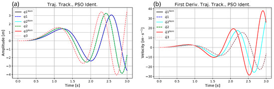
Figure 3.
Trajectory tracking (a) and the first time derivatives (b) for the three robot links in the parameter identification process.
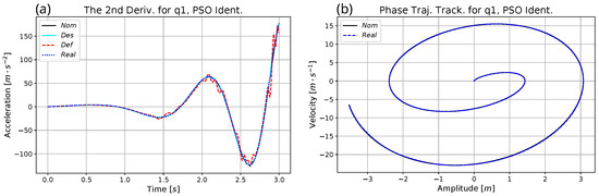
Figure 4.
The second time derivatives (a) and phase trajectory tracking (b) for .
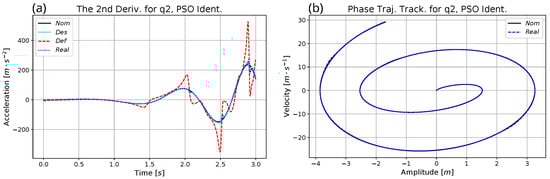
Figure 5.
The second time derivatives (a) and phase trajectory tracking (b) for .
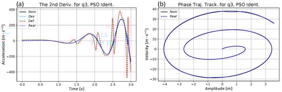
Figure 6.
The second time derivatives (a) and phase trajectory tracking (b) for .
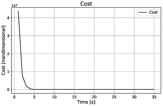
Figure 7.
The cost function of the best estimation of the model during PSO teaching iteration.
The accuracy of each estimated value for each targeted parameter is shown in Figure 8. For revealing the estimation accuracy in the five-dimensional parameter space, Figure 9 and Figure 10 display the story of the “best global particle” in various 2D projections.
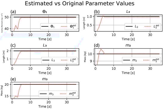
Figure 8.
The estimated vs original parameters during teaching iteration (a) for (b) for (c) for (d) for (e) for .
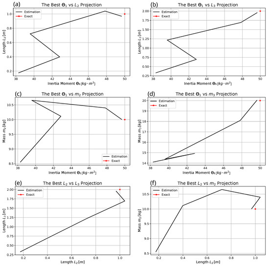
Figure 9.
Projection of the estimated elements (a) vs. (b) vs. (c) vs. (d) vs. (e) vs. (f) vs. .
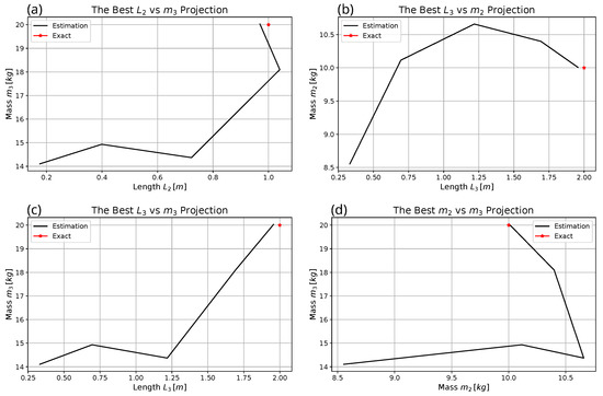
Figure 10.
Projection of the estimated elements (a) vs. (b) vs. (c) vs. (d) vs. .
5.2. Operation of the Non-Adaptive CTC vs. Adaptive CTC for the Identified Parameters
After identifying the appropriate parameters by PSO, a natural option would be using the common non-adaptive CTC in the possession of the identified model. However, the computations revealed that the small errors in the identified parameters are not completely insignificant. It may be advantageous to maintain the adaptive controller even in the case in which the identified dynamic parameters are used. For this reason, two versions of the CTC controller were applied: one without any adaption technique, while the other by activating the FPI-based adaptive mechanism. It can be expected that the effect of adaptivity will be more significant in the identification phase when a very imprecise model will be used for tracking a prescribed trajectory. It can be expected that its significance will not be so great when a more precise model will be in use.
In fact, the trajectory tracking error in the PSO-based identifying process was between and whereas it increased in non-adaptive CTC within the range . The better improvement was in the adaptive CTC within the range . The same holds for the first derivative trajectory tracking error. It increased from in the original identifying process to in non-adaptive CTC. The error decreased to in adaptive CTC. The comparison can be seen in Figure 11, Figure 12 and Figure 13. The detailed explanation and interpretation of these observations are discussed in the sequel in Section 6.
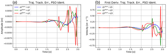
Figure 11.
Trajectory tracking error (a) and its first time derivative (b) during the parameter identification process.
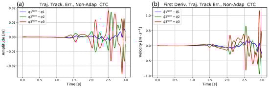
Figure 12.
Trajectory tracking error (a) and its first time derivative (b) for the non-adaptive CTC controller using the identified parameters.
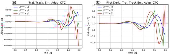
Figure 13.
Trajectory tracking error (a) and its first time derivative (b) for the adaptive CTC controller using the identified parameters.
6. Discussion
Since in the case of the control of a second order system the essence of the FPI-based adaptive control is the “deformation of the second time derivatives”, the details of the figures conveying information on that of the nominal trajectory as , , , the “Desired” values as , , , the “Deformed” ones as , , , and the “Realized” terms as , , have to be investigated.
In general, it can be expected that in the case of an imprecise model the non-adaptive controller has to apply significant PID error correction terms to the second time derivatives of the nominal coordinates; therefore, in this case, quite considerable differences can be expected between the values of , , , and , , : the significant additions in the desired terms have the role of making the necessary corrections in the non-adaptive controller. For a good operation, the “Realized” values should well track these “Desired” ones, but this cannot be well realized in the non-adaptive controller. The limited applicability of the non-adaptive controller consists in this fact. However, when the adaptation mechanism is in use, it is expected that the “Realized” value better approximates the “Desired” one, consequently the necessary PID-type corrections in the “Desired” term continuously decrease in time, therefore both the “Desired” and the “Realized” values converge to the “Nominal” ones, while the “Deformed” ones can increase accordingly. (As the final results, the precision of trajectory tracking and that of the first time derivatives of the generalized coordinates can be compared by the use of Figure 11, Figure 12 and Figure 13. It can be seen that the non-adaptive controller that uses the identified parameters has the greatest error, the “second greatest error” belongs to the adaptive CTC controller using the original data, and finally, the most precise tracking was achieved by the adaptive controller using the identified model parameters.)
The above-mentioned effects can be well observed in the simulation results when the not completely precise identified parameters were used in the non-adaptive and adaptive versions of the CTC controller. This effect can be well tracked in the “zoomed-in excerpts” of Figure 14 and Figure 15 for the coordinate .
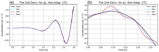
Figure 14.
Second time derivatives for (a) and the zoomed-in excerpts (b) for the non-adaptive CTC controller using the identified parameters.
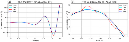
Figure 15.
Second time derivatives for (a) and the zoomed-in excerpts (b) for the adaptive CTC controller using the identified parameters.
Similar effects can be well identified in Figure 16 and Figure 17 for the coordinate , and in Figure 18 and Figure 19, for the coordinate , too.
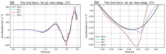
Figure 16.
Second time derivatives for (a) and the zoomed-in excerpts (b) for the non-adaptive CTC controller using the identified parameters.
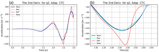
Figure 17.
Second time derivatives for (a) and the zoomed-in excerpts (b) for the adaptive CTC controller using the identified parameters.
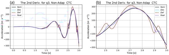
Figure 18.
Second time derivatives for (a) and the zoomed-in excerpts (b) for the non-adaptive CTC controller using the identified parameters. The results of the simulation investigations generate conclusions detailed in Section 7.
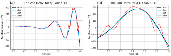
Figure 19.
Second time derivatives for (a) and the zoomed-in excerpts (b) for the adaptive CTC controller using the identified parameters.
Though for the very imprecise initial model no non-adaptive simulations were done, in Figure 20, Figure 21 and Figure 22, similar observations can be done for the coordinates , , and , respectively. The adaptive controller brought closer to each other the , , and values by applying a considerable extent of adaptive deformations.
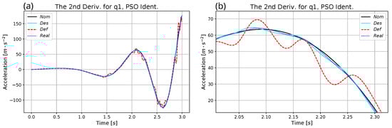
Figure 20.
Second time derivatives for (a) and the zoomed-in excerpt (b) during the parameter identification process.
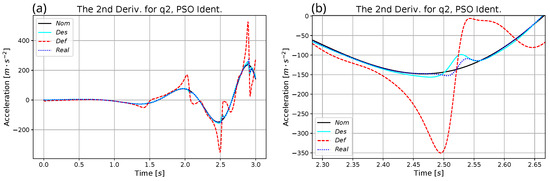
Figure 21.
Second time derivatives for (a) and the zoomed-in excerpt (b) during the parameter identification process.
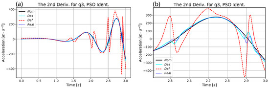
Figure 22.
Second time derivatives for (a) and the zoomed-in excerpt (b) during the parameter identification process.
A possible “measure of extent of adaptive deformation” is the angle of abstract rotation in this special adaptive controller. Figure 23 underpins the fact that: the use of the very imprecise model during the parameter identification process needed a much more drastic adaptive deformation than the adaptive use of the identified parameters.
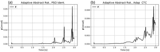
Figure 23.
The angle of adaptive abstract rotation during the parameter identification process (a), and for the adaptive CTC controller using the identified parameters (b).
In the previous sections, the operation of the controllers was illustrated by zoomed-in excerpts of appropriate figures. For a more exact comparison, the use of the measures of operation can be introduced:
that is the average tracking error , the average 1st derivative tracking error , and the average second derivative error in which the Manhattan distance-based norm was in use in the case of second derivative the error is not a tracking error but the difference between the “desired” and the “Realized” values. The computational results for the average errors are given in Table 2:

Table 2.
Comparison of the various error measurements.
From the previous Table 2 it can be seen that, in general, in the adaptive control more accurate trajectory tracking, i.e., less average tracking error was achieved than in the case of the non-adaptive approach. Furthermore, in the case of the improved model the trajectory tracking error became even less. For example, in the case of using the Approximate Model, adaptivity made the average trajectory tracking error decrease approximately by the factor times that of its non-adaptive counterpart. While in the case of the Improved Model it decreased by approximately times. The difference in accuracy using the adaptive activation between the approx model and improved model is 1:1.2 (regarding the favor of the last). The same can be said for the average first derivative of the trajectory tracking error and the average second derivative tracking error. The error decreased, respectively, by 0.3201 and 0.1 times by adaptivity in the case of the Approximate Model. In addition to the ratio of 1:1.12 for the first derivative, and the ratio of 1:2.55 for the second derivative of the adaptive controllers when the Approximate Model was replaced by the Improved Model.
The results of the simulation investigations generated conclusions detailed in Section 7.
7. Conclusions
The most important conclusion can be that, by using the PSO algorithm, it is easy to achieve a relatively precise identification of the model parameters, the effects of the remaining imprecisions cannot be completely neglected. Since the FPI-based adaptive technique can be well combined with evolutionary methods to achieve improved efficiency (e.g., [72]), the application of this adaptive technique seems to be promising.
Regarding the usefulness of parameter identification by PSO—adaptive deformations that are too big may cause problems in the floating point representation of the numbers in the computers. These problems can be evaded if the necessary adaptive deformations can be reduced, i.e., when the initial approximate model is relatively precise because it is identified by PSO-based processes.
For future work, the possible problem involving measurement noises (in connection with the FPI-based control) deserves attention. The noise effects were not investigated in this simulation study; they can be the subjects of detailed investigations.
Presently, preparations are taking place to test the adaptive method experimentally by using industrial controller components instead of simple Arduino-based units on a mechanical test engine made of the components of a real robot. It is expected that the higher speeds of these control units will make it possible to study the effects of such drastic nonlinear effects (as sticking) that can be modeled by quite sophisticated friction models.
The bases of our expectations are based on the nature of the FPI-based control method outlined in Figure 1. In general, the speed of convergence of the method can be increased by decreasing the cycle time of the digital controller; this speed directly concerns the available precision of the controller. Furthermore, in the adaptive deformation, some “delay” (normally the cycle time of the controller) is applied. If the dynamics of the controlled system are very fast, during this delay time, the observed model can become obsolete by the time of the next control cycle. These properties of the FPI-based adaptation seriously concern the possible efficiency of such controllers.
This adaptive approach in principle is applicable in higher-order and higher relative order controllers, in which higher derivatives of 2 must be observed. A typical case is when a quantity that should be controlled by the physically available control force is connected to the action point of the force through the connected subsystem. In such cases, the computations of the higher derivatives need a lot of mathematical operations, i.e., the computations of various Lie derivatives. Instead of using the time to compute them, they can be approximated by the use of simple affine terms, and the errors caused by them can be adaptively compensated. The “goodness” of this affine approximation concerns the necessary steps of the Banach iteration; in this manner, it also concerns the precision of the trajectory tracking. Instead of complicated theoretical considerations, experiments and measurements can give reliable answers to the range of applicability of this control method.
Author Contributions
Conceptualization, H.I.; software, H.I.; validation, J.K.T.; Formal analysis, J.K.T.; writing—original draft preparation, J.K.T.; writing—review and editing, H.I.; supervision, J.K.T. All authors have read and agreed to the published version of the manuscript.
Funding
This research received no external funding.
Institutional Review Board Statement
Not applicable.
Informed Consent Statement
Not applicable.
Data Availability Statement
Not applicable.
Acknowledgments
The authors highly acknowledge the support from the Doctoral School of Applied Informatics and Applied Mathematics, Óbuda University Budapest, Hungary.
Conflicts of Interest
The authors declare that they have no conflict of interest.
References
- Corke, P.; Armstrong-Helouvry, B. A Search for Consensus Among Model Parameters Reported for the PUMA 560 Robot. In Proceedings of the 1994 IEEE International Conference on Robotics and Automation, San Diego, CA, USA, 8–13 May 1994; pp. 1608–1613. [Google Scholar]
- Andoga, R.; Főző, L. Near Magnetic Field of a Small Turbojet Engine. Acta Phys. Pol. 2017, 131, 1117–1119. [Google Scholar] [CrossRef]
- Andoga, R.; Főző, L.; Schrötter, M.; Češkovič, M.; Szabo, S.; Bréda, R.; Schreiner, M. Intelligent Thermal Imaging-Based Diagnostics of Turbojet Engines. Appl. Sci. 2019, 9, 2253. [Google Scholar] [CrossRef]
- Spodniak, M.; Főző, L.; Andoga, R.; Semrád, K.; Beneda, K. Methodology for the Water Injection System Design Based on Numerical Models. Acta Polytech. Hung. 2021, 18, 47–62. [Google Scholar] [CrossRef]
- Andoga, R.; Főző, L.; Judičák, J.; Bréda, R.; Szabo, S.; Rozenberg, R.; Džunda, M. Intelligent Situational Control of Small Turbojet Engines. Int. J. Aerosp. Eng. 2018, 2018, 1–16. [Google Scholar] [CrossRef]
- Andoga, R.; Főző, L.; Kovács, R.; Beneda, K.; Moravec, T.; Schreiner, M. Robust Control of Small Turbojet Engines. Machines 2019, 7, 3. [Google Scholar] [CrossRef]
- Slotine, J.J.E.; Li, W. Applied Nonlinear Control; Prentice Hall International, Inc.: Englewood Cliffs, NJ, USA, 1991. [Google Scholar]
- Lyapunov, A. A General Task about the Stability of Motion. Ph.D. Thesis, University of Kazan, Tatarstan, Russia, 1892. (In Russian). [Google Scholar]
- Lyapunov, A. Stability of Motion; Academic Press: New York, NY, USA; London, UK, 1966. [Google Scholar]
- Lin, H.; Zhao, B.; Liu, D.; Alippi, C. Data-based fault tolerant control for affine nonlinear systems through particle swarm optimized neural networks. IEEE/CAA J. Autom. Sin. 2020, 7, 954–964. [Google Scholar] [CrossRef]
- Wang, D.; Liu, S.; He, Y.; Shen, J. Barrier Lyapunov function-based adaptive back-stepping control for electronic throttle control system. Mathematics 2021, 9, 326. [Google Scholar] [CrossRef]
- Chen, H.; Haus, B.; Mercorelli, P. Extension of SEIR compartmental models for constructive Lyapunov control of COVID-19 and analysis in terms of practical stability. Mathematics 2021, 9, 2076. [Google Scholar] [CrossRef]
- Nguyen, C.; Antrazi, S.; Zhou, Z.L.; Campbell, C.E., Jr. Adaptive Control of a Stewart Platform-based Manipulator. J. Robot. Syst. 1993, 10, 657–687. [Google Scholar] [CrossRef]
- Banach, S. Sur les opérations dans les ensembles abstraits et leur application aux équations intégrales (About the Operations in the Abstract Sets and Their Application to Integral Equations). Fund. Math. 1922, 3, 133–181. [Google Scholar] [CrossRef]
- Tar, J.; Bitó, J.; Nádai, L.; Machado, J.T. Robust Fixed Point Transformations in Adaptive Control Using Local Basin of Attraction. Acta Polytech. Hung. 2009, 6, 21–37. [Google Scholar]
- Tar, J.; Bitó, J.; Rudas, I. Replacement of Lyapunov’s Direct Method in Model Reference Adaptive Control with Robust Fixed Point Transformations. In Proceedings of the 2010 IEEE 14th International Conference on Intelligent Engineering Systems, Las Palmas of Gran Canaria, Spain, 5–7 October 2010; pp. 231–235. [Google Scholar]
- Varga, A.; Kovács, L.; Eigner, G.; Kocur, D.; Tar, J.K. Fixed Point Iteration-based Adaptive Control for a Delayed Differential Equation Model of Diabetes Mellitus. In Proceedings of the 2019 IEEE International Conference on Systems, Man and Cybernetics (SMC), Bari, Italy, 6–9 October 2019; pp. 1408–1413. [Google Scholar] [CrossRef]
- Issa, H.; Tar, J.K. Preliminary Design of a Receding Horizon Controller Supported by Adaptive Feedback. Electronics 2022, 11, 1243. [Google Scholar] [CrossRef]
- Faitli, T. Investigation of Control Methods for a Speed-Controlled Electric Motor. Bachelor’s Thesis, Óbuda University, Donát Bánki Faculty of Mechanical and Safety Engineering, Institute of Mechatronics and Autotechnics, Budapest, Hungary, 2018. [Google Scholar]
- Armstrong, B.; Khatib, O.; Burdick, J. The Explicit Dynamic Model and Internal Parameters of the PUMA 560 Arm. In Proceedings of the 1986 IEEE International Conference on Robotics and Automation, San Francisco, CA, USA, 7–10 April 1986; pp. 510–518. [Google Scholar]
- Varga, A.; Eigner, G.; Rudas, I.; Tar, J. Experimental and Simulation-Based Performance Analysis of a Computed Torque Control (CTC) Method Running on a Double Rotor Aeromechanical Testbed. Electronics 2021, 10, 1745. [Google Scholar] [CrossRef]
- Bodó, Z.; Lantos, B. Integrating Backstepping Control of Outdoor Quadrotor UAVs. Period. Polytech.–Electr. Eng. Comput. Sci. 2019, 63, 122–132. [Google Scholar] [CrossRef]
- Dumetz, E.; Dieulot, J.Y.; Barre, P.J.; Colas, F.; Delplace, T. Control of an Industrial Robot using Acceleration Feedback. J. Intell. Robot. Syst. 2006, 46, 111–128. [Google Scholar] [CrossRef]
- Wang, Q.; Cai, H.X.; Huang, Y.M.; Ge, L.; Tang, T.; Su, Y.R.; Liu, X.; Li, J.Y.; He, D.; Du, S.P.; et al. Acceleration feedback control (AFC) enhanced by disturbance observation and compensation (DOC) for high precision tracking in telescope systems. Res. Astron. Astrophys. 2016, 16, 124. [Google Scholar] [CrossRef]
- Hamandi, M.; Tognon, M.; Franchi, A. Direct acceleration feedback control of quadrotor aerial vehicles. In Proceedings of the 2020 IEEE International Conference on Robotics and Automation (ICRA), Paris, France, 31 May–31 August 2020; pp. 5335–5341. [Google Scholar]
- Tar, J.; Bitó, J.; Várkonyi-Kóczy, A.; Dineva, A. Symbiosys of RFPT-based Adaptivity and the Modified Adaptive Inverse Dynamics Controller. In Advances in Soft Computing, Intelligent Robotics and Control; Fodor, J., Fullér, R., Eds.; Springer: Heidelberg, Germany; London, UK; New York, NY, USA, 2014; pp. 95–106. [Google Scholar]
- Tar, J.; Rudas, I.; Dineva, A.; Várkonyi-Kóczy, A. Stabilization of a Modified Slotine-Li Adaptive Robot Controller by Robust Fixed Point Transformations. In Proceedings of the International Conference on Intelligent Control, Modelling and Systems Engineering, 2014, Cambridge, MA, USA, 29–31 January 2014; pp. 35–40. [Google Scholar]
- Lagrange, J.; Binet, J.; Garnier, J. Mécanique Analytique (Analytical Mechanics); Binet, J.P.M., Garnier, J.G., Eds.; Ve Courcier: Paris, France, 1811. [Google Scholar]
- Gambár, K.; Márkus, F. A possible dynamical phase transition between the dissipative and the non-dissipative solutions of a thermal process. Phys. Lett. A 2007, 361, 283–286. [Google Scholar] [CrossRef]
- Gambár, K.; Lendvay, M.; Lovassy, R.; Bugyjás, J. Application of Potentials in the Description of Transport Processes. Acta Polytech. Hung. 2016, 13, 173–184. [Google Scholar]
- Bellman, R. Dynamic Programming and a new formalism in the calculus of variations. Proc. Natl. Acad. Sci. USA 1954, 40, 231–235. [Google Scholar] [CrossRef]
- Kalman, R. Contribution to the Theory of Optimal Control. Bol. Soc. Mat. Mex. 1960, 5, 102–119. [Google Scholar]
- Nelder, J.; Mead, R. A simplex method for function minimization. Comput. J. 1965, 7, 308–313. [Google Scholar] [CrossRef]
- Dantzig, G. Origins of the Simplex Method (Technical Report Sol 87-5); Systems Optimization Laboratory, Department of Operations Research, Stanford University: Stanford, CA, USA, 1987. [Google Scholar]
- Galántai, A. A convergence analysis of the Nelder-Mead simplex method. Acta Polytech. Hung. 2021, 18, 93–105. [Google Scholar] [CrossRef]
- Kirkpatrick, S.; Gelatt, C.D., Jr.; Vecchi, M.P. Optimization by simulated annealing. Science 1983, 220, 671–680. [Google Scholar] [CrossRef]
- Moscato, P. On Evolution, Search, Optimization, Genetic Algorithms and Martial Arts: Towards Memetic Algorithms. Caltech Concurrent Computation Program, Report 826; Caltech: Pasadena, CA, USA, 1989. [Google Scholar]
- Szénási, S.; Felde, I. Configuring Genetic Algorithm to Solve the Inverse Heat Conduction Problem. Acta Polytech. Hung. 2017, 14, 133–152. [Google Scholar]
- Földesi, P.; Botzheim, J.; Kóczy, L. Eugenic bacterial memetic algorithm for fuzzy road transport traveling salesman problem. Int. J. Innov. Comput. 2009, 7, 2775–2798. [Google Scholar]
- Botzheim, J.; Toda, Y.; Kubota, N. Bacterial memetic algorithm for simultaneous optimization of path planning and flow shop scheduling problems. Artif. Life Robot. 2012, 17, 107–112. [Google Scholar] [CrossRef]
- Botzheim, J.; Toda, Y.; Kubota, N. Bacterial memetic algorithm for offline path planning of mobile robots. Memetic Comput. 2012, 4, 73–86. [Google Scholar] [CrossRef]
- Zamani, H.; Nadimi-Shahraki, M.H.; Gandomi, A.H. Starling murmuration optimizer: A novel bio-inspired algorithm for global and engineering optimization. Comput. Methods Appl. Mech. Eng. 2022, 392, 114616. [Google Scholar] [CrossRef]
- Mirjalili, S. Moth-flame optimization algorithm: A novel nature-inspired heuristic paradigm. Knowl. Based Syst. 2015, 89, 228–249. [Google Scholar] [CrossRef]
- Nadimi-Shahraki, M.H.; Fatahi, A.; Zamani, H.; Mirjalili, S.; Abualigah, L. An improved moth-flame optimization algorithm with adaptation mechanism to solve numerical and mechanical engineering problems. Entropy 2021, 23, 1637. [Google Scholar] [CrossRef]
- Zamani, H.; Nadimi-Shahraki, M.H.; Gandomi, A.H. QANA: Quantum-based avian navigation optimizer algorithm. Eng. Appl. Artif. Intell. 2021, 104, 104314. [Google Scholar] [CrossRef]
- Bajec, I.; Heppner, F. Organized flight in birds. Anim. Behav. 2009, 78, 777–789. [Google Scholar] [CrossRef]
- Kennedy, J.; Eberhart, R. Particle swarm optimization. In Proceedings of the ICNN’95-International Conference on Neural Networks, Perth, WA, USA, 27 November–1 December 1995; Volume 4, pp. 1942–1948. [Google Scholar]
- Felde, I.; Szénási, S. Estimation of temporospatial boundary conditions using a particle swarm optimisation technique. Int. J. Microstruct. Mater. Prop. 2016, 11, 288–300. [Google Scholar] [CrossRef]
- Le, L.T.; Nguyen, H.; Zhou, J.; Dou, J.; Moayedi, H. Estimating the heating load of buildings for smart city planning using a novel artificial intelligence technique PSO-XGBoost. Appl. Sci. 2019, 9, 2714. [Google Scholar] [CrossRef]
- Le, L.T.; Nguyen, H.; Dou, J.; Zhou, J. A comparative study of PSO-ANN, GA-ANN, ICA-ANN, and ABC-ANN in estimating the heating load of buildings’ energy efficiency for smart city planning. Appl. Sci. 2019, 9, 2630. [Google Scholar] [CrossRef]
- Ahmadi, M.; Soofiabadi, M.; Nikpour, M.; Naderi, H.; Abdullah, L.; Arandian, B. Developing a deep neural network with fuzzy wavelets and integrating an inline PSO to predict energy consumption patterns in urban buildings. Mathematics 2022, 10, 1270. [Google Scholar] [CrossRef]
- Nabi, S.; Ahmad, M.; Ibrahim, M.; Hamam, H. AdPSO: Adaptive PSO-based task scheduling approach for cloud computing. Sensors 2022, 22, 920. [Google Scholar] [CrossRef]
- Sung, W.T.; Tsai, M.H. Data fusion of multi-sensor for IOT precise measurement based on improved PSO algorithms. Comput. Math. Appl. 2012, 64, 1450–1461. [Google Scholar] [CrossRef]
- Liu, G.; Zhu, Y.; Xu, S.; Chen, Y.C.; Tang, H. PSO-based power-driven X-routing algorithm in semiconductor design for predictive intelligence of IoT applications. Appl. Soft Comput. 2022, 114, 108114. [Google Scholar] [CrossRef]
- Liu, J.; Fang, H.; Xu, J. Online Adaptive PID control for a multi-joint lower extremity exoskeleton system using improved particle swarm optimization. Machines 2021, 10, 21. [Google Scholar] [CrossRef]
- Xu, L.; Song, B.; Cao, M. An improved particle swarm optimization algorithm with adaptive weighted delay velocity. Syst. Sci. Control. Eng. 2021, 9, 188–197. [Google Scholar] [CrossRef]
- Vijay, M.; Jena, D. PSO based neuro fuzzy sliding mode control for a robot manipulator. J. Electr. Syst. Inf. Technol. 2017, 4, 243–256. [Google Scholar] [CrossRef]
- Chu, Z.; Ma, Y.; Cui, J. Adaptive reactionless control strategy via the PSO-ELM algorithm for free-floating space robots during manipulation of unknown objects. Nonlinear Dyn. 2018, 91, 1321–1335. [Google Scholar] [CrossRef]
- Sharma, K.D.; Chatterjee, A.; Rakshit, A. A PSO–Lyapunov hybrid stable adaptive fuzzy tracking control approach for vision-based robot navigation. IEEE Trans. Instrum. Meas. 2012, 61, 1908–1914. [Google Scholar] [CrossRef]
- Rastrigin, L. Systems of Extremal Control; Mir: Moscow, Russia, 1974. [Google Scholar]
- Rudolph, G. Globale Optimierung mit Parallelen Evolutionsstrategien (Diplomarbeit) Global Optimization with Parallel Evolution Strategies. Master’s Thesis, Department of Computer Science, University of Dortmund, Dortmund, Germany, 1990. [Google Scholar]
- Weierstraß, K. Über continuirliche Functionen eines reellen Arguments, die für keinen Werth des letzeren einen bestimmten Differentialquotienten besitzen, (On single variable continuous functions that nowhere are differentiable). In Königlich Preussichen Akademie der Wissenschaften, Mathematische Werke von Karl Weierstrass; Mayer & Mueller: Berlin, Germany, 1895; Volume 2, pp. 71–74. [Google Scholar]
- Tarantola, A. Inverse Problem Theory and Methods for Model Parameter Estimation; Society for Industrial and Applied Mathematics (SIAM): Philadelphia, PA, USA, 2005. [Google Scholar]
- Dunik, J.; Simandl, M.; Straka, O. Unscented Kalman filter: Aspects and adaptive setting of scaling parameter. IEEE Trans. Autom. Control 2012, 57, 2411–2416. [Google Scholar] [CrossRef]
- Menegaz, H.M.; Ishihara, J.A.Y.; Borges, G.A.; Vargas, A.N. A systematization of the unscented Kalman filter theory. IEEE Trans. Autom. Control 2015, 60, 2583–2598. [Google Scholar] [CrossRef]
- Kuti, J.; Galambos, P. Decreasing the Computational Demand of Unscented Kalman Filter based Methods. In Proceedings of the 2021 IEEE 15th International Symposium on Applied Computational Intelligence and Informatics (SACI), Timișoara, Romania, 19–21 May 2021; pp. 181–186. [Google Scholar]
- Varga, B.; Tar, J.; Horváth, R. Tuning of Dynamic Model Parameters for Adaptive Control Using Particle Swarm Optimization. In Proceedings of the IEEE 10th Jubilee International Conference on Computational Cybernetics and Cyber-Medical Systems ICCC 2022, Reykjavík, Iceland, 6–9 July 2022; Szakál, A., Ed.; IEEE Hungary Section: Budapest, Hungary, 2022; pp. 197–202. [Google Scholar]
- Issa, H.; Tar, J.K. On the Limitations of PSO in Cooperation with FPI-based Adaptive Control for Nonlinear Systems. In Proceedings of the Accepted for publication in: 2022 IEEE 26th International Conference on Intelligent Engineering Systems (INES), Crete, Greece, 12–15 August 2022; pp. 0001–0006. [Google Scholar]
- van der Pol, B. Forced oscillations in a circuit with non-linear resistance (reception with reactive triode). Lond. Edinb. Dublin Philos. Mag. J. Sci. 1927, 7, 65–80. [Google Scholar] [CrossRef]
- Csanádi, B.; Galambos, P.; Tar, J.; Györök, G.; Serester, A. A Novel, Abstract Rotation-based Fixed Point Transformation in Adaptive Control. In Proceedings of the 2018 IEEE International Conference on Systems, Man, and Cybernetics (SMC), Miyazaki, Japan, 7–10 October 2018; pp. 2577–2582. [Google Scholar]
- Dineva, A. Non-Conventional Data Representation and Control. Ph.D. Thesis, Óbuda University, Budapest, Hungary, 2016. [Google Scholar]
- Lovas, I. Fixed Point Iteration-based Adaptive Controller Tuning Using a Genetic Algorithm. Acta Polytech. Hung. 2022, 19, 59–77. [Google Scholar] [CrossRef]


Publisher’s Note: MDPI stays neutral with regard to jurisdictional claims in published maps and institutional affiliations. |
© 2022 by the authors. Licensee MDPI, Basel, Switzerland. This article is an open access article distributed under the terms and conditions of the Creative Commons Attribution (CC BY) license (https://creativecommons.org/licenses/by/4.0/).