Abstract
Constitutional processes are a cornerstone of modern democracies. Whether revolutionary or institutionally organized, they establish the core values of social order and determine the institutional architecture that governs social life. Constitutional processes are themselves evolutionary practices of mutual learning in which actors, regardless of their initial political positions, continuously interact with each other, demonstrating differences and making alliances regarding different topics. In this article, we develop Tree Augmented Naive Bayes (TAN) classifiers to model the behavior of constituent agents. According to the nature of the constituent dynamics, weights are learned by the model from the data using an evolution strategy to obtain a good classification performance. For our analysis, we used the constituent agents’ communications on Twitter during the installation period of the Constitutional Convention (July–October 2021). In order to differentiate political positions (left, center, right), we applied the developed algorithm to obtain the scores of 882 ballots cast in the first stage of the convention (4 July to 29 September 2021). Then, we used k-means to identify three clusters containing right-wing, center, and left-wing positions. Experimental results obtained using the three constructed datasets showed that using alternative weight values in the TAN construction procedure, inferred by an evolution strategy, yielded improvements in the classification accuracy measured in the test sets compared to the results of the TAN constructed with conditional mutual information, as well as other Bayesian network classifier construction approaches. Additionally, our results may help us to better understand political behavior in constitutional processes and to improve the accuracy of TAN classifiers applied to social, real-world data.
1. Introduction
On the afternoon of 18 October 2019, serious riots took place in different parts of Santiago, Chile. Within hours, the situation escalated into the most important Chilean political event of the 21st century, with massive and violent protests that lasted for about a month. In order to avoid the collapse of the democratic system, the government and political forces from across the ideological spectrum called for a peace agreement and a new constitution. This paved the way for the institutional organization of the demands through a new constitution [1,2].
After the reorganization of the electoral calendar due to COVID-19, the first session of the Constitutional Convention, in charge of writing the new Chilean Constitution, took place on 4 July 2021. The convention consisted of 155 members, with equal numbers of seats for women and men, and with a quota of 17 seats reserved for native peoples. Politically, it was composed of 37 right-wing, 36 center-left, 54 left-wing, and 11 independent members (mostly left-wing members), as well as 17 representatives of native peoples.
The convention agenda provided three months for the creation of the rules of procedures and nine months for the elaboration of the substantive content of the constitution. Thus, the new constitution should be delivered by the convention in July 2022 and ratified (or rejected) by the people in a final plebiscite. On 29 September 2021, the convention approved its General Rules, and on 18 October 2021 (exactly two years after the 2019 riots), it began to discuss the substantive contents of the constitution.
In this article, we focus on analyzing the opinions posted on Twitter by the convention members during the constitutional process. In particular, we used a non-structured dataset composed of the Twitter posts of 135 out of the 155 members (20 did not have a Twitter account) of the Constitutional Convention between 4 July and 27 October 2021. This amounts to 37,814 tweets. In order to differentiate the members’ political positions (left, center, right), we applied a nominate algorithm [3] to obtain the scores of 882 ballots cast in the first stage of the convention (4 July to 29 September 2021). This algorithm was originally developed for the analysis of U.S. congressional votes and has been applied in multiple political contexts. As a multidimensional scaling technique, its fundamental objective is to project high-dimensional data (voting patterns) to a low-dimensional space for the purpose of interpretation. In particular, this involves projection to a dimension with the voting behavior of a specific political group—in this case, the members of the Chilean Constitutional Convention. According to whether they vote in favor, against, or abstain, the convention members are given a score between −1 and 1 which positions them in a graphic space. Those who vote similarly are then placed closer in the distribution; when they differ, they are placed farther from each other. Based on this, it is assumed that those members situated below 0 hold a “left-wing” political position, while those who are positioned above 0 have a “right-wing” political position. Then, we used k-means to identify three clusters containing right-wing, center, and left-wing positions. These positions have to be considered to be relative to the political distribution within the convention—i.e., they depend on the voting behavior of the members. Members classified as “center” tended to be from center-left political parties (social democracy, socialist party), while the “left-wing” members of the convention were mainly members of the Communist Party, independents, and indigenous people.
For sentiment classification for each cluster, we were interested in using a classifier with interpretability capabilities and good classification performance; therefore, we explored different Bayesian network classifiers that have been successfully applied in other sentiment classification applications [4].
The rest of the paper is organized as follows. Section 2 presents a brief overview of Bayesian networks, Bayesian network classifiers, and recent sentiment analysis approaches. The Twitter data acquisition, description, pre-processing, sentiment classification, and proposed learning approach for the Bayesian network classifier is presented in Section 3. The results and analysis are discussed in Section 4. Finally, the conclusions of this work as well as future research are given in Section 5.
2. Background
2.1. Bayesian Networks
Bayesian networks were first introduced by Judea Pearl [5] for joint probability computation. These are probabilistic graphical models that represent discrete random variables and their conditional dependencies via a directed acyclic graph (DAG). Originally, Bayesian networks were constructed by hand using human domain knowledge, but then it became of interest to develop algorithms to learn the networks from data [6,7]. Learning Bayesian networks from data has two components: (1) the structure of the networks and (2) the parameters (conditional probability tables). Unfortunately, the work in [8] proved that learning Bayesian networks from data is NP-complete. Therefore, it has been of interest to develop approximate learning approaches to simplify the learning process [9,10]. For (1), the search can be carried out through an evolutionary computation approach. Some examples include: the combination of genetic algorithms with particle swarm optimization (PSO) called Breeding Swarm to learn Bayesian networks [11], an artificial bee colony (ABC) algorithm for learning Bayesian networks [12], and learning Bayesian networks using a genetic algorithm [13,14]. A review of evolutionary computation approaches for learning Bayesian networks can be found in [15].
In classification (supervised learning) problems, when adopting a probabilistic approach the challenge is to effectively compute the posterior probability of the class variable (with ) given an n-dimensional input data point . This can be achieved using the Bayes rule:
In particular, it is of interest the numerator, which contains the product of the a priori probability of the class variable and the likelihood, which corresponds to the joint probability of the input features conditioned to the class variable. The computation of the a priori probability of the class variable is straightforward. It can be obtained through the relative frequency of the class variable values in the training set. Still, there are many approaches that can be used for computing the likelihood. One of these is to use Bayesian networks, giving way to Bayesian network classifiers [16]. Recent applications of Bayesian network classifiers include sentiment analysis using Twitter data [4], facial biotype prediction for orthodontic treatment planning [17], obstructive sleep apnea diagnosis [18], movie recommender systems [19], air quality forecasting [20], the detection of keratoconus (thinning of the cornea and irregularities of the cornea’s surface) [21], fault diagnosis [22], breast cancer diagnosis [23], and the detection of hydrothermal alteration zones associated with epithermal gold mineralization [24].
Amongst the many versions of Bayesian network classifiers [25,26,27,28,29,30], the two most popular are the naive Bayesian network classifier [31] and the Tree Augmented Naive Bayes (TAN) classifier [16]. The naive Bayes version assumes conditional independence amongst the attributes given the class variable to compute the likelihood in (1). Therefore, there are no edges between the attributes, as shown in the example in Figure 1. Improvements to the naive Bayes include feature weighting techniques [32,33], boosted parameter learning [34], and the exact learning augmented naive Bayes classifier [35].
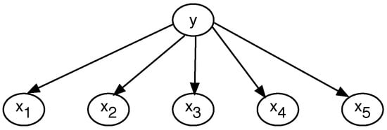
Figure 1.
Example of the naive Bayesian network classifier.
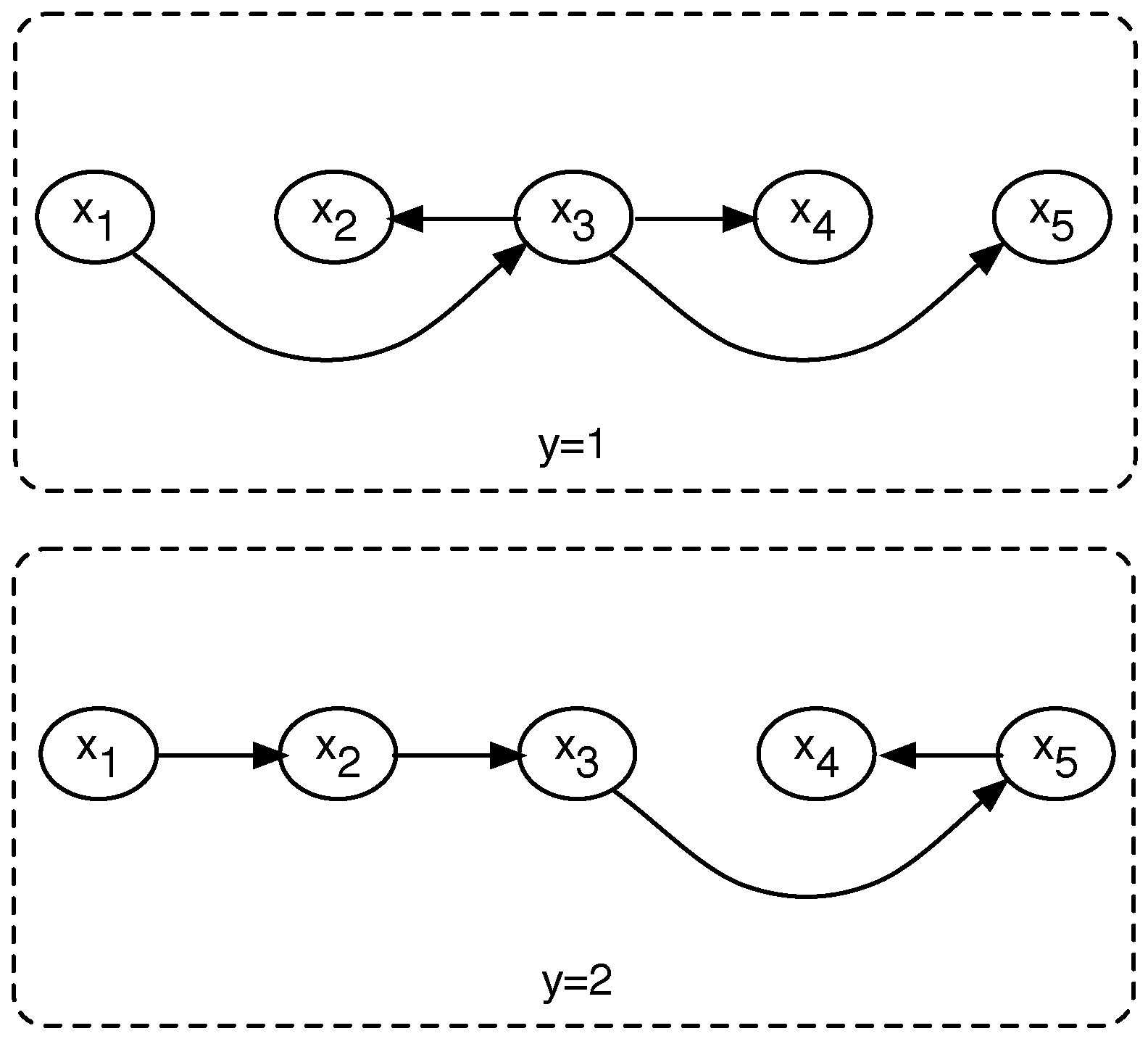
Whereas TAN starts off by considering a fully connected network where the edges have weights, these are computed using the conditional mutual information between pairs of attributes. Then, the maximum weighted spanning tree (MWST) method, similar to Kruskal’s algorithm [36], is applied to obtain a tree structure, leaving only edges. Under this version of a Bayesian network classifier, each attribute will have one incoming edge from another attribute, except for the chosen root attribute node. Of course, just like the naive Bayesian network classifier, in the TAN model, in addition to the tree structure, each node will have an incoming edge from the class variable, as shown in the example of Figure 2.
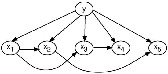
Figure 2.
Example of the TAN classifier.
The TAN model corrects the strong assumption of conditional independence established by the naive version. In theory, it should produce better results (accuracy) than the naive Bayes classifier. However, TAN suffers from some problems—one, in particular, is the ability to provide a correct estimate of the conditional mutual information. The conditional mutual information is a measure from information theory that corresponds to a generalization of the correlation, which is also capable of capturing linear and non-linear relationships. In particular, for two variables and , the conditional mutual information for these two attributes given the class is given by [37]:
measures the information that provides about when the value of is known, and is non-negative. A main difficulty when working with mutual information or conditional mutual information is when there is not a sufficient number of training examples per class to estimate the joint probability distribution and the conditional distributions in (2) correctly, meaning that the resulting conditional mutual information estimate is not so reliable. This is critical, since TAN obtains its tree structure using as weights in the fully connected graph. From this, a natural question arises: can the weights of the network be learned directly from the data to obtain good classification results without having to estimate the conditional mutual information in (2)?
2.2. Tree Augmented Naive Bayes Classifiers
The TAN classifier is based on the seminal work of Chow and Liu [38], who presented a method to approximate the joint probability distribution of a set of variables, imposing a tree structure as a model of dependencies amongst the variables. The development starts off by using the Kullback–Leibler divergence as a measure to quantify how different one distribution is from another. Let be the real probability distribution of and let be an approximation of the real distribution. Then, the matter of how close is to can be quantified through :
The idea is to minimize (3). For this, Chow and Liu consider that has a tree structure as a model of dependencies amongst the variables. With some algebraic manipulations and the use of information theory definitions, (3) can be rewritten as:
where is the mutual information between variable and its parent , is the entropy of variable , and ) is the joint entropy of the variable set . By inspecting (4), one can see that and are independent of the tree structure amongst the variables. Only is dependent of the tree structure, and since it is a non-negative measure and there is a minus sign in front of the sum of the mutual information between the edges of the tree structure, minimizing is equivalent to maximizing . Therefore, the Chow–Liu tree procedure is as follows:
- Build a fully connected weighted graph where the nodes are the variables/attributes of your problem and the weights of the edges are the mutual information between pairs of nodes.
- Apply a maximum spanning tree algorithm to obtain a tree structure amongst the variables, such that the sum of weights is the maximum. Here, Kruskal’s algorithm can be used for this purpose.
- Transform the undirected tree to a directed one by choosing a root variable and then setting the direction of all edges to face outward from it.
In the context of classification, we can partition the training set into subgroups containing only examples from the same class. Then, we can use the Chow–Liu tree algorithm to infer the joint probability of the input features (variables) for each class, and use this as the likelihood in (1) to see for which class the input data point obtains the highest posterior probability. An example of the Chow–Liu tree classifier for a two-class problem is shown in Figure 3.
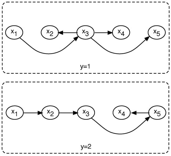
Figure 3.
Example of the Chow–Liu tree classifier.
The TAN classifier is an upgrade of the Chow–Liu tree algorithm, where instead of having to train a tree for each class, TAN uses conditional mutual information (2). Therefore, it is only necessary to train one tree for all the classes. The TAN procedure is as follows:
- Build a fully connected weighted graph where the nodes are the variables/attributes of your problem and the weights of the edges are the conditional mutual information between pairs of nodes.
- Apply a maximum spanning tree algorithm, to obtain a tree structure amongst the variables, such that the sum of weights is maximum. Here, Kruskal’s algorithm can be used for this purpose.
- Transform the undirected tree to a directed one by choosing a root variable and then setting the direction of all edges to be outward from it.
- Construct a TAN model by adding a vertex labelled y and adding an edge from y to each .
As we can see, the resulting tree structure, and, therefore, the likelihood used in (1) to compute the posterior probability, depends of the weight values used in step (1). If we change the weights, this may lead to a different structure and thus a different posterior probability and eventually a different classification of an example. Therefore, in this work we propose an alternative learning method to infer the weights to use in step (1) of the TAN procedure, such that we obtain a high classification performance. For this, we adopt an optimization procedure based on the evolution strategy described in Section 3.6. Other improvements or variants of TAN include averaging TAN models (called ATAN) resulting from considering each node as the root node (step 3 of the TAN procedure) [39], generalizing TAN from 1-dependence Bayesian network classifier to arbitrary k-dependence [40], and an attribute selective approach for TAN that builds a sequence of approximate models using only the top certain attributes [41].
2.3. Recent Sentiment Analysis Approaches
Although the focus of this paper is the use of Bayesian network classifiers in the context of sentiment analysis, another recent approach includes a stance classification system for Twitter data related to vaccination in Italy which uses term frequency-inverse document frequency (TF-IDF) for the representation of numerical features (the same as we do in this paper) and a support vector machine (SVM) with a linear kernel as the classification model [42]. When different data sources are combined (multimodal data) to carry out sentiment analysis, the important problem of missing values may appear, which is also known as the modality missing issue. In [43], the modality missing issue is addressed by proposing a modality distillation method based on a tensor fusion network. For the problem of intent classification for dialogue utterances, ref. [44] investigated several machine learning methods, concluding that SVM obtained the best results based on the macro-F1 metric. Ref. [45] presents a sentiment analysis study focusing on topics and emotions in video car reviews from YouTube; in this analysis, an SVM was used as the classification model. In [46], a review of major emotion models is conducted and a new version of the Hourglass model, which is a biologically inspired and psychologically motivated emotion categorization model for sentiment analysis, is proposed.
Rumors on Twitter are investigated in [47], where a two-stage methodology that combines a hierarchical long short-term memory (LSTM) network with the various classifiers—SVM, naive Bayes, decision trees, and multilayer perceptron—is presented. In [48], a stacked ensemble of shallow convolutional neural networks (CNNs) is proposed for tracking the moods, emotions, and sentiments of patients expressing an intake of medicine in Twitter. Sentiment and sarcasm classification are tackled in [49] via a multitask learning-based framework using a deep neural network, outperforming a state-of-the-art method based on a CNN. In [50], different deep-learning-based architectures are explored for multimodal sentiment classification, with the bc-LSTM model obtaining the best results. In [51], a new version of SenticNet called SenticNet 6 is proposed; this is built using an approach to knowledge representation that is both top-down and bottom-up via an ensemble of symbolic and subsymbolic AI tools that are applied to the problem of polarity detection from text.
A mathematical explanation of neural tensor network (NTN) is given in [52], as well as the inner link between NTN and other models—e.g., feedforward neural network and attention mechanism—from the perspective of Taylor’s theorem. The empirical studies performed on sentiment analysis, named entity recognition and knowledge base completion tasks, provided some valuable insights into NTN. In particular, it was found that the 1st-order NTN achieves a competitive performance in most cases.
In cases where the text that has been analyzed contains more than one opinion target and therefore sentiment analysis is not treated as a binary classification problem, ref. [53] introduces a convolutional stacked bidirectional long short-term memory with a multiplicative attention mechanism for aspect category and sentiment polarity detection that treats the sentiment analysis as a multiclass classification problem. The proposed model was evaluated using the SemEval-2015 and SemEval-2016 datasets, outperforming state-of-the-art methods in aspect-based sentiment analysis.
3. Data and Methods
3.1. Twitter Data
Tweets from the 135 convention members with a Twitter account (out of the 155) were collected using the Twitter API between 4 July and 27 October 2021. This amounts to 37,814 tweets, including 497,715 total words, of which 33,832 are unique words.
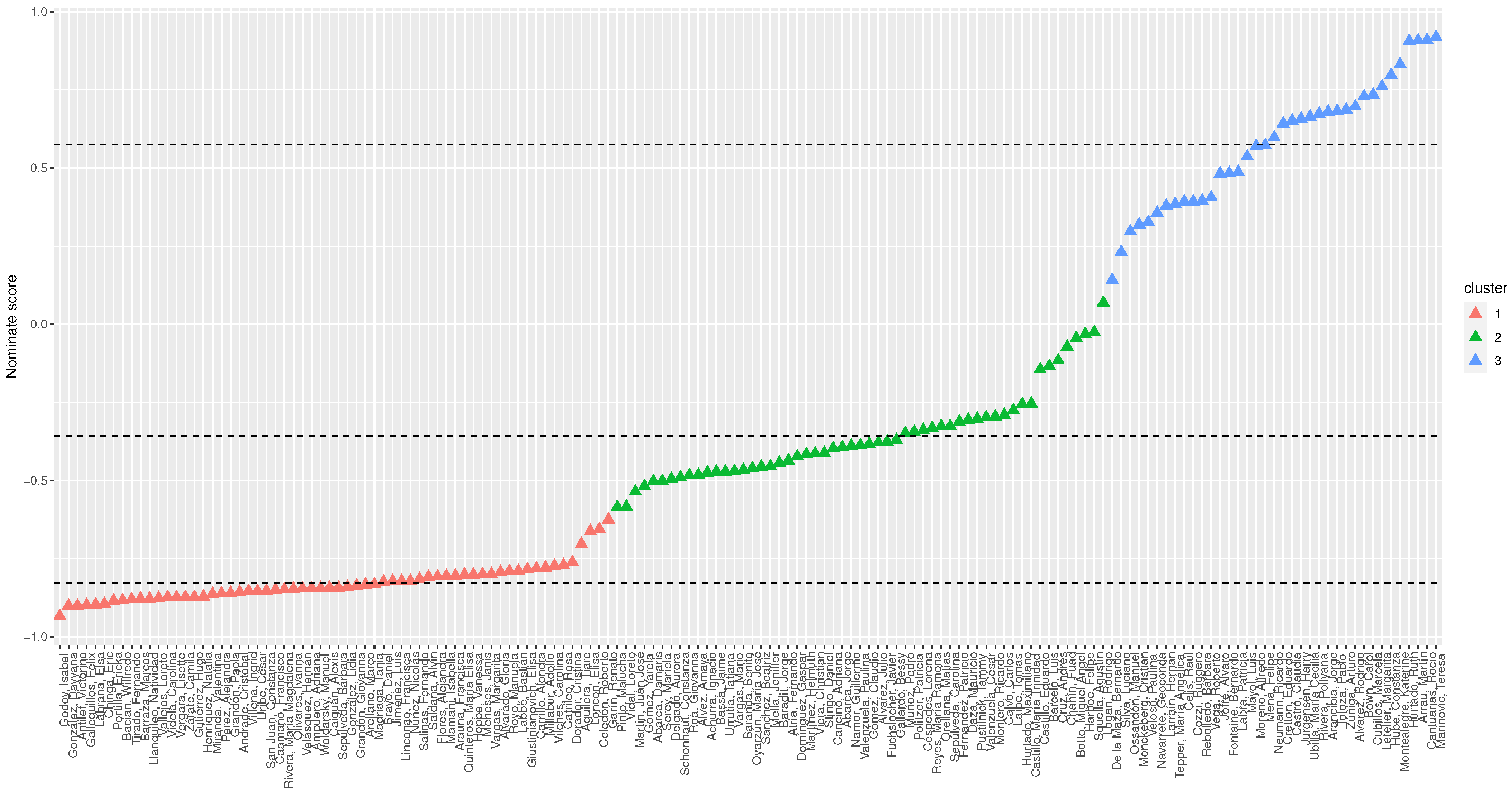
To analyze these tweets, we grouped the Twitter accounts differentiating political positions (left, center, right) with the nominate algorithm [3]. We applied the algorithm to 882 ballots cast in the first stage of the convention (from 4 July to 29 September 2021). Then, we used k-means to identify three clusters containing left-wing (cluster 1), center (cluster 2), and right-wing positions (cluster 3). These positions have to be considered to be relative to the political distribution within the convention—i.e., they depend on the voting behavior of the members.
The nominate scores and the clusters found by k-means with are shown in Figure 4.
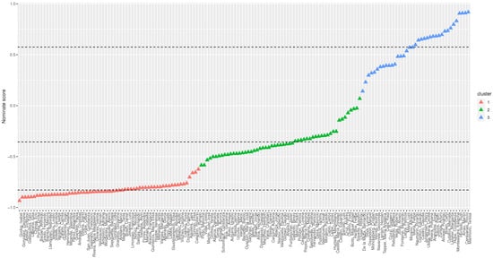
Figure 4.
Nominate score.
Table 1 presents the Twitter accounts and the number of tweets grouped by the their political positions (clusters).

Table 1.
Clusters and Twitter accounts.
Finally, the time series representing the total number of tweets per hour and cluster are shown in Figure 5.
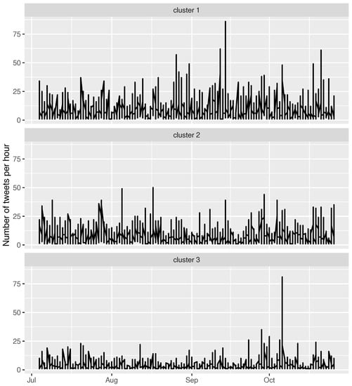
Figure 5.
Time series representing the total number of tweets per hour.
3.2. Pre-Processing
Raw data are highly susceptible to inconsistency and redundancy. The pre-processing of tweets is necessary and includes the following points:
- Removing all URLs (e.g., www.xyz.com), hashtags (e.g., #topic), and targets (@username);
- Removing all punctuation, symbols, and numbers;
- Correcting the spellings and handling the sequence of repeated characters;
- Removing stop words;
- Removing non-Spanish tweets.
3.3. Term Frequency-Inverse Document Frequency (TF-IDF)
The TF-IDF method determines the relative frequency of words in a specific document through an inverse proportion of the word over the entire document corpus. For determining the value, the method uses two elements: TF, the term frequency of the term i in the document j, and IDF, the inverse document frequency of the term i. TF-IDF can be calculated as [54]:
where is the weight of term i in a document j, N is the number of documents in the collection, is the term frequency of the term i in a document j, and is the document frequency of the term i in the collection.
The resulting TF-IDF matrices for each cluster were, 17,192 for cluster 1, 14,502 for cluster 2, and for cluster 3. These will be the datasets used to train and test the classifiers.
3.4. Sentiment Analysis
In the previous subsection, we described how the input data matrices were constructed. Now, we need the class labels. These were obtained as follows.
Each tweet was labeled with a sentiment with two possible values: negative or positive. We used a list of English positive and negative opinion words or sentiment words (around 7000 words) [55], which we translated into Spanish. In this article, we first determined the sentiment polarity of each tweet by adapting the following measure [4]:
The sentiment score has the range , where ‘positive’ represents the positive word count and ‘negative’ represents the negative word count in a tweet. Sometimes, we cannot decide the degree of emotionality of a tweet because the polarity measure fails to do so () or the positives and negatives cancel each other out. In this case, we cannot decide whether the tweet is positive, negative, or neutral. Therefore, we introduced the following definition:
where C is the class label of the tweet being analyzed.
By applying the above methodology, we obtained the following class labels:
- Cluster 1: 12,298 negative tweets (−1) and 4894 positive tweets (1);
- Cluster 2: 9761 negative tweets (−1) and 4741 positive tweets (1);
- Cluster 3: 4518 negative tweets (−1) and 1602 positive tweets (1).
Usually, in many sentiment analysis classification models, neutral comments are not considered [56,57]. There are two main reasons for this: (1) these models focus on binary classification—i.e., in the identification of positive versus negative opinions; (2) neutral comments lack information due to their ambiguity.
Neutrality means the absence of sentiment or no sentiment [58]. Neutral comments show an ambiguous weight of sentiment—i.e., they contain an equitable burden of positive and negative polarity [59].
Due to this, this category has been considered as noisy and is broadly excluded from many sentiment models [60,61,62,63]. However, some researchers have tackled the problem of neutrality: the authors in [57] propose taking into account neutral reviews in order to improve the classification results, and the authors in [64] propose the use of a multi-sentiment scale, 1–5 stars, to solve the problem of obtaining a wider range of sentiment representation. It is understood that detecting and removing noise can improve a model’s performance [59].
In future work, we will consider studying the neutral tweets to improve the binary polarity classification using TAN classifiers.
3.5. Model Performance Evaluation
We evaluated four measures: precision (), recall (), accuracy (), and -score. These measures are computed as follows:
where , , , and denote true positive, true negative, false positive, and false negative, respectively.
3.6. An Evolution Strategy for Learning TAN Classifiers
An evolution strategy (ES) is an iterative (generational) procedure. In each generation, new individuals (offspring) are created from existing individuals (parents). The canonical versions of the ES are denoted by:
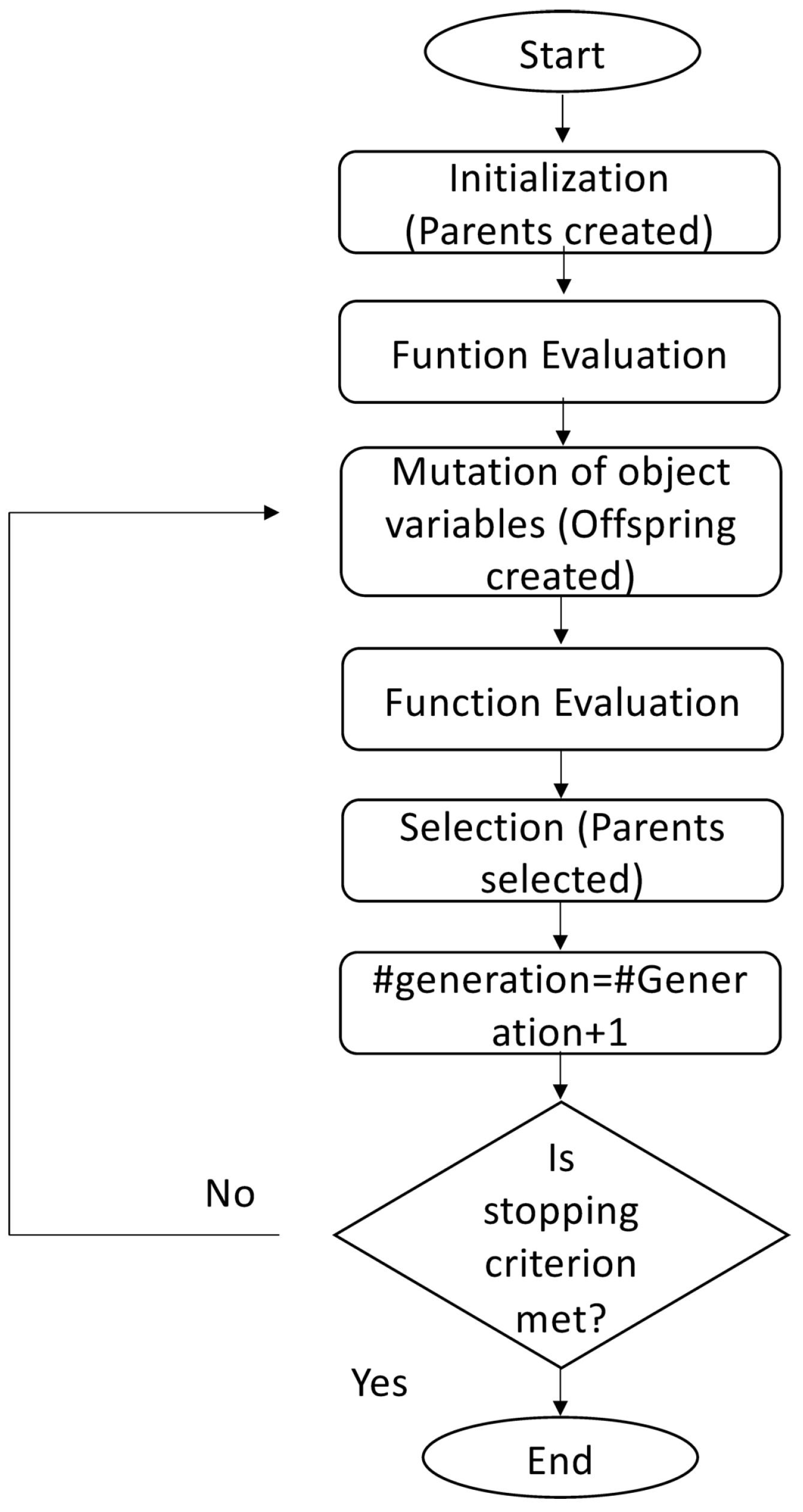
Here, denotes the number of parents and denotes the number of offspring. The parents are deterministically selected (i.e., deterministic survivor selection) from the multi-set of either the offspring, referred to as comma selection ( must hold), or both the parents and offspring, referred to as plus selection. Selection is based on the ranking of the individuals’ fitness, taking the best individuals (also referred to as truncation selection). Figure 6 is a flowchart that briefly describes how the ES algorithm works. The interested reader is referred to [65] for more details on how ES works.

Figure 6.
Flowchart of the evolution strategy.
We propose to use the deterministic survivor selection method to obtain weights for the TAN model, which yields good classification results without estimating the conditional mutual information.
Since the TAN learning procedure starts with a fully connected weighted graph, for a network with n nodes we need to define weights. Therefore, for the cluster 1 dataset with 133 attributes (words), we need to find 8778 weights (parameters). For the cluster 2 dataset, which has 130 attributes, we need to find 8385 weights, and for the cluster 3 dataset, with 172 attributes, we need to find 14,706 weights. To find the appropriate values for these weights for each dataset, we proceed independently as follows.
An individual is a candidate solution coded as an m-dimensional vector containing the m weight values of a network. We generate an initial population of individuals by placing all the weight values uniformly at random in the unit hypercube for each individual. Next, we iterate over a fixed number of iterations of the algorithm. Each iteration first involves evaluating each candidate solution in the population.
Then, we calculate the fitness function using the fraction of correctly classified examples (in the training set), which is also known as the accuracy.
Next, we select the parents with the best scores, which are the highest scores in this case, as we are maximizing the objective function. We consider the following steps:
- The parent population contains individuals.
- denotes the number of offspring generated in each iteration.
- Individuals die out after one iteration step (we use 1000 iterations), and only the offspring (the youngest individuals) survive to the next generation. In that case, environmental selection chooses parents from offspring.
These hyperparameters were chosen after trial and error simulations.
3.7. Experimental Setup
We compared the performance of the naive Bayesian network classifier (NB), original TAN, Averaged TAN (ATAN) [39] described in Section 2.2, and the proposed method -TAN. In addition, we implemented four greedy hill-climbing algorithms for learning Bayesian network classifiers:
- Hill-climbing tree augmented naive Bayes (HC-TAN) [66].
- Hill-climbing super-parent tree augmented naive Bayes (HC-SP-TAN) [66].
- Backward sequential elimination and joining (BSEJ) [25].
- Forward sequential selection and joining (FSSJ) [25].
The HC-TAN and HC-SP-TAN algorithms start from a naive Bayes structure and add edges until there is no improvement in the network score. BSEJ starts from a naive Bayes structure and adds augmenting edges; it then removes features from the model until no improvement in the network score is witnessed. On the contrary, FSSJ starts from a structure containing just the class node and proceeds by incorporating features and augmenting edges.
For each dataset (cluster), we run the data splitting procedure 10 times, with 70% used for training and 30% used for testing (the splitting was carried out randomly). For each run, we computed the four classification performance measures on the test set, after which the average and the standard deviation of each measure was reported.
All the simulations were carried out using the open-source R software environment for statistical computing.
4. Results and Analysis
The results, when considering the accuracy measure, are shown in Table 2. Overall, we notice that -TAN outperforms TAN in the three datasets, particularly for the cluster 3 and cluster 1 datasets, where more than a 5% increase in accuracy score was obtained. When compared to NB, significant improvements were obtained for the three datasets—again, particularly for cluster 3 and cluster 1, where a more than 8% increase in accuracy score was achieved. Compared to the hill-climbing approaches, we notice that -TAN outperforms HC-TAN and HC-SP-TAN for all the datasets. This also holds when compared to BSEJ and FSSJ. ATAN, an improvement of TAN, obtains similar results to HC-TAN, HC-SP-TAN, and BSEJ.
Table 2.
Performance comparison of NB, TAN, ATAN, HC-TAN, HC-SP-TAN, BSEJ, FSSJ, and -TAN in terms of accuracy in the test set.
In general, we notice that the lowest performance for all the classifiers is for the cluster 3 dataset. This is mainly due to an overfitting phenomenon, since more weights need to be found than the existing amount of training examples. Nevertheless, -TAN outperforms TAN in accuracy by 6%.
When looking at the precision measure results in Table 3, we notice that -TAN outperforms all the other classifiers for all the datasets. Moreover, -TAN was the only model that obtained precision values above 92% for the three datasets. This analysis also holds for the recall measure shown in Table 4 and the -score shown in Table 5, where -TAN was the only classifier that obtained recall values above 81% and -score values above 86%, respectively, for the three datasets.
Table 3.
Performance comparison of NB, TAN, ATAN, HC-TAN, HC-SP-TAN, BSEJ, FSSJ, and -TAN in terms of precision in the test set.
Table 4.
Performance comparison of NB, TAN, ATAN, HC-TAN, HC-SP-TAN, BSEJ, FSSJ, and -TAN in terms of recall in the test set.
Table 5.
Performance comparison of NB, TAN, ATAN, HC-TAN, HC-SP-TAN, BSEJ, FSSJ, and -TAN in terms of -score in the test set.
These results support our hypothesis that the TAN can infer better trees for classification purposes. This is achieved by replacing the computation of conditional mutual information with some other weights learned from the data specifically to enhance the classification performance.
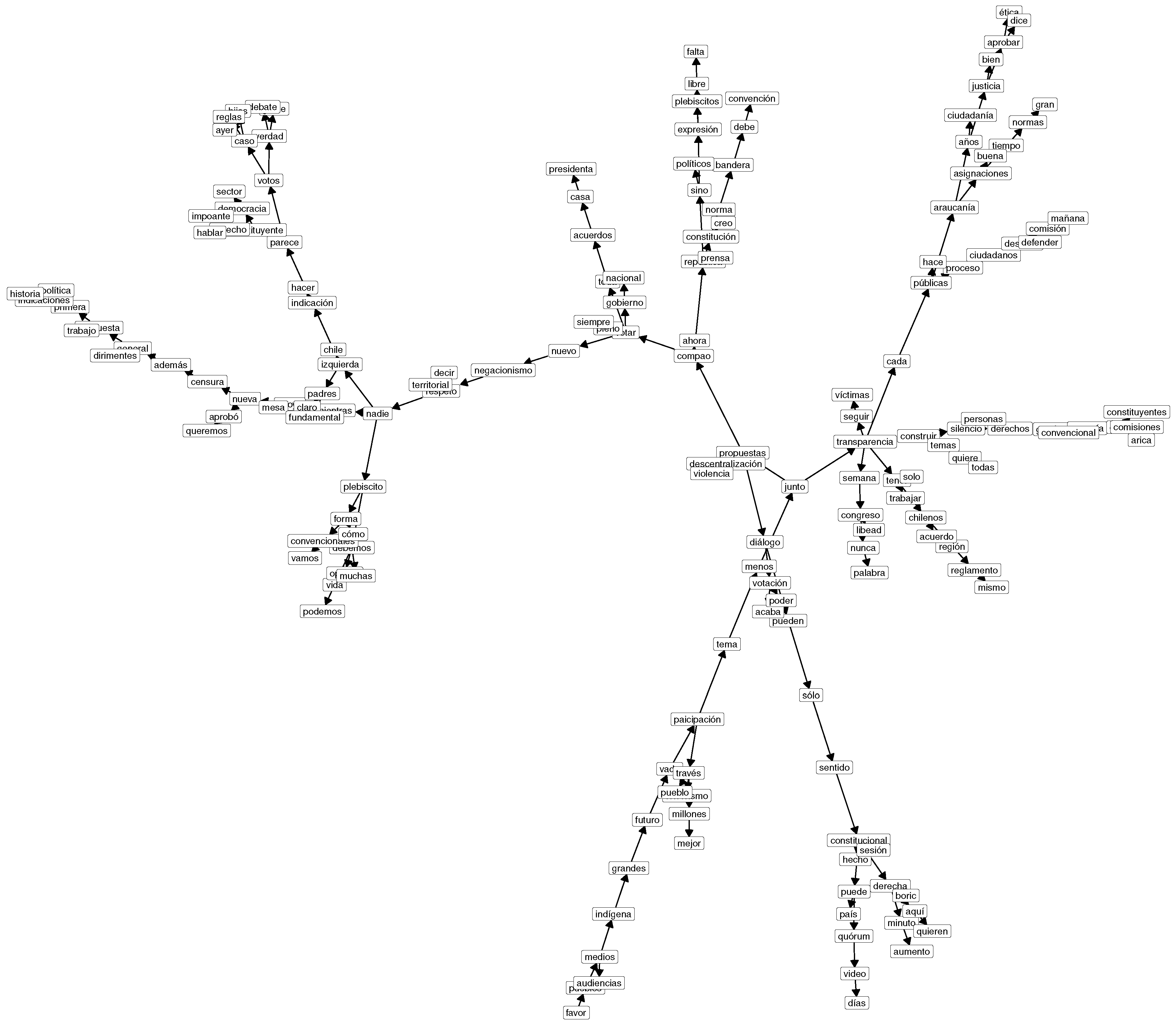
Examples of the resulting networks using -TAN are shown in Figure 7 for the cluster 1 dataset, Figure 8 for the cluster 2 dataset, and Figure 9 for the cluster 3 dataset. For better visualization, in these figures we omitted the node with the class variable and the edges from this node to all the other nodes.
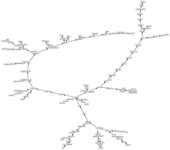
Figure 7.
Examples of solutions achieved using -TAN for the cluster 1 dataset.
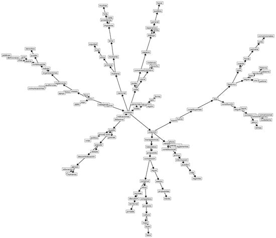
Figure 8.
Examples of solutions achieved using -TAN for the cluster 2 dataset.
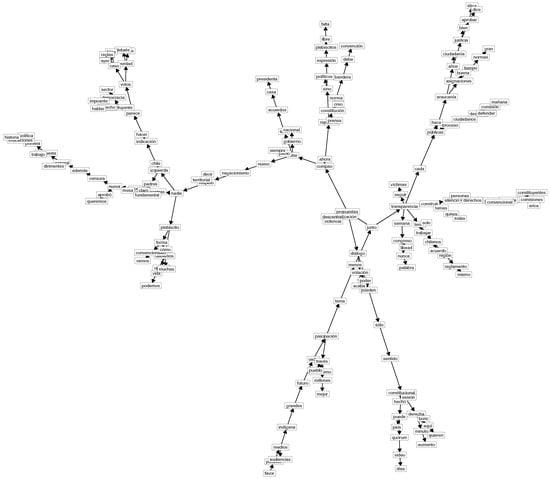
Figure 9.
Examples of solutions achieved using -TAN for the cluster 3 dataset.
Interpreting the Networks
Bayesian networks classifiers offer not only a quantitative mode of analysis but also a significant qualitative view of the data, particularly when dealing with Twitter communication.
For this qualitative approach to data, we analyze the three networks representing different political positions within the Chilean Constitutional Convention. Through the aforementioned procedure (see Section 3), we obtain a behavioral classification of the political attitudes of the members and not self-declarative positioning. In this classification (see Figure 4), we obtain a network for left-wing positions in cluster 1 (Figure 7), one for central positions in cluster 2 (Figure 8), and one for right-wing positions in cluster 3 (Figure 9).
Considering Figure 7, we observe several politically meaningful terms and directed edges for a rather identitarian left-wing view (independent movements, Communist Party, indigenous people). Terms such as “pueblo”, indígena (indigenous), mujeres (women), popular (popular), and octubre (October) reflect central concerns for the rather radical left-wing members of the convention. “October” refers to 18 October 2019, the day the popular uprising began. A very common self-description in left-wing Latin American politics consists of distinguishing between the elite and “pueblo”. In this case, the category of “pueblo” does not really mean “the people”, as in the U.S. American constitution, in which the term works as an inclusive category of citizenship. In Latin American semantic usage, “people” is a category that is construed for grouping historically discriminated-against actors [67]. It includes women, indigenous people, workers, among others—i.e., the “popular world” (as expressed in the network), which is opposed to the category of “elites”, made up of privileged, well-educated, modern citizens. This division of the world between “pueblo” and “elite” is rather common in Latin American left-wing populism (Argentina, Venezuela, Bolivia, Ecuador, Cuba) and constitutes the ideological basis for constructing a hegemonic strategy of political access to state power [68].
In this case, it is worth mentioning three directed edges: (a) popular → Chile; (b) apoyo (support) → territorial, and apoyo (support) → social; (c) Mapuche → originarios; and (d) normas → indígena (indigenous) → convencionales (members of the convention). The directed edge (a) condenses the idea of a country (Chile) belonging to the popular classes, which is semantically combined with the directed edge (b), referring to the territorial and social support for the construction of this new order. The project of a popular nation began to grow after the critical events of 18 October 2019. Left-wing political parties aimed at reconstructing the events (protests, riots, violent demonstrations) as a popular demand for justice and political changes that would reverse the current state of affairs in which elites prevail, thereby transforming Chile into a “popular republic” (popular → Chile)—i.e., a country that belongs “to the pueblo”. In this scenario, indigenous people such as the Mapuche (from southern Chile) play a crucial role: as original inhabitants of the country, they represent the precolonial essence of the popular nation in left-wing politics [69]. For this reason, indigenous peoples have been granted reserved seats (escaños) in the convention (see the directed edge pueblo → escaños). Of the 155 seats, 17 have been exclusively granted to representatives of indigenous peoples, the majority of whom are Mapuche.
Considering Figure 8, in which a view of center-left politicians is represented (mostly from the social democracy and socialist party), we also observe meaningful terms and directed edges related to this political approach. Terms such as equidad (equity), diálogo (dialogue), democracia (democracy), transparencia (transparency), derechos (rights), ddhh (abb. for human rights), abd ciudadanía (citizenship) are classical concerns and principles of social democratic parties in modern liberal democracies. The discourse concerning rights and human rights is the most general framework for this political view. According to this, the discourse around rights and human rights is not only an institutional discourse but also heuristic meaningful semantics through which people conceive their daily experience in the social world and articulate their demands of both the government and institutions [70]. This expresses the success of the modern narrative of rights and, at the same time, reinforces universal democratic values such as equity, dialogue, democracy, transparency, and citizenship—namely, the core of social democratic politics.
According to this, in Figure 8, we observe some interesting directed edges: (a) conversando (conversation) → espacio (space) → diálogo (dialogue) → esperanza (hope), as well as the bifurcation diálogo (dialogue) → general → pueblos (people); (b) votación (ballots) → transparencia (transparency) → convención (convention); (c) trabajo (work) → constituyente (member of the convention) → pueblo (people) → derechos (rights); and (d) Chile → democracy (democracia) → públicas (policy). In this case, the network construction reveals a rather liberal conception of democracy in which, through spaces of conversation and dialogue, the hopes of the people can be addressed [71]. The transparency of democratic procedures is also mentioned in the network, as well as the (hard) work carried out by the Constitutional Convention for the rights of Chilean “pueblo” (people). Unlike what happens in the case of the network of the radical left-wing members of the convention, the concept of “pueblo” must now be comprehended within a different semantic constellation that refers to the democratic conditions of citizenship, as expressed in the directed edge (a) and in the above-described relevant single terms. This is an inclusive and universal concept of “pueblo” understood as rights-based citizenship, which is common in U.S. American and European politics. Finally, the directed edge chile → democracia (democracy) → públicas (policy), refers to the policies (políticas públicas) that should implement rights that would lead to achieving citizenship. To that extent, policies are closely connected to democracy in the view of the center-left members of the convention.
Figure 9 represents the view of the right-wing members of the Chilean Constitutional Convention (liberal and social conservative parties). A rather common behavior in right-wing politics consists of constructing a dual vision of the political field. On the one hand, right-wing members affirm their own values, and, on the other, they express criticism of the principles and attitudes of left-wing politics [72]. The network mirrors this duality with terms affirming right-wing values, such as libertad (liberty), libre (free), expresión (expression), diálogo (dialogue), and bandera (flag), and terms referring to critical concerns, such as censura (censorship), izquierda (left), violencia (violence), and víctimas (victims). With these references, the right-wing members of the convention conduct an affirmative political strategy of their own positions and, at the same time, oppose the more left-wing stances.
We find a similar situation when we observe the directed edges. We identify four relevant edges: (a) nueva (new) → censura (censorship); (b) nuevo (new) → negacionismo (denial); (c) expresión (expression) → plebiscitos (plebiscite) → free (libre); and (d) trabajar (work) → chilenos (Chilean) → acuerdo (agreement) → reglamento (regulation). Directed edges (a) and (b) oppose the proposals made by the left-wing members of the convention aimed at limiting freedom of expression (control of the media and the proposal of ’denial by omission’, which implies the mandatory recognition of human rights violations every time the events of October 2019 are discussed); meanwhile, directed edges (c) and (d) express the affirming attitude of right-wing members regarding freedom of expression and the orientation towards agreements regarding the formulation of the convention’s rules of procedure.
As can be seen, the classification offers a meaningful and detailed view of the qualitative political dynamics of the members of the Chilean Constitutional Convention. It allows us to recognize distinctive semantic elements in left-wing, center, and right-wing politics that not only describe the static components of the process, but also the mutual references between political positions, as well as their substantive foundations (values, principles) and political strategies (self-affirmation, opposition, criticism).
5. Conclusions
These results confirmed our view that the tree structures obtained using conditional mutual information do not necessarily yield the best classifiers. Moreover, based on the number of features and training samples, the performance of the TAN classifier can be quite affected, as shown in the case of the cluster 3 dataset.
Another drawback when using conditional mutual information is that the resulting tree might not be reliable for interpretability purposes, a topic that is quite popular nowadays. Indeed, one of the advantages of using Bayesian network classifiers is the possibility of interpreting and understanding the classification process and the results by analyzing the network and how the features interact. For example, when analyzing the resulting network for the cluster 1 dataset, the TAN model achieved a mean accuracy value of 76 versus 81 when using -TAN. Furthermore, even though the -TAN model showed the lowest performance in cluster 3 (due to overfitting) with a mean accuracy of 79, it significantly outperformed the TAN model, which showed a mean accuracy of 73. Which network is more reliable for interpreting the results? Common sense warns that the model with the best performance should have a more reliable network, with interactions or dependencies that are more realistic than those in a model with a lower performance. This is something that could be tested in future research with artificially generated data.
Considering our qualitative interpretation of the networks, we can conclude that the resulting tree structures offer analytically interesting material with which to understand the political behavior and semantics of the members of the Chilean Constitutional Convention. These results present politically meaningful words and directed edges that allow for a differentiation between left-wing, center, and right-wing positions both ideologically (through principles and values) and in terms of political practices (self-affirmation, opposition, and criticism). The qualitative interpretation could even contribute to explaining the lower mean accuracy value of the -TAN in cluster 3 (right-wing members of the Chilean Constitutional Convention), in addition to the overfitting. The composition of this network is more complex than that of others, as right-wing members apply a dual strategy of self-affirmation and criticism of left-wing positions, thus using terms with both a right-wing identity (self-affirmation) and a left-wing identity (for criticizing the left). Therefore, the model needs more training examples to increase its accuracy in this case. Further research should test this conjecture.
Here, we have used a simple evolution strategy in the model to learn the weights. Of course, other evolutionary computation techniques could also be used to test other hybrid algorithms. Future research should consider more benchmark datasets as well as industrial applications.
Author Contributions
Conceptualization, G.A.R., P.A.H. and A.M.; methodology, G.A.R., P.A.H. and A.M.; software, P.A.H.; validation, G.A.R., P.A.H. and A.M.; formal analysis, G.A.R., P.A.H. and A.M.; investigation, G.A.R., P.A.H. and A.M.; resources, G.A.R. and A.M.; data curation, P.A.H.; writing—original draft preparation, G.A.R., P.A.H. and A.M.; writing—review and editing, G.A.R., P.A.H. and A.M.; visualization, G.A.R., P.A.H. and A.M.; supervision, G.A.R., P.A.H. and A.M.; project administration, G.A.R., P.A.H. and A.M.; funding acquisition, G.A.R. and A.M. All authors have read and agreed to the published version of the manuscript.
Funding
The authors would like to thank ANID FONDECYT grant number 1180706 (G.A.R), ANID FONDECYT grant number 1190265 (A.M., G.A.R.), and ANID PIA/BASAL FB0002 (G.A.R.) for financially supporting this research.
Institutional Review Board Statement
Not applicable.
Informed Consent Statement
Not applicable.
Data Availability Statement
The data presented in this study are available on request from the corresponding author.
Acknowledgments
The authors would like to thank the research assistant Carolina Molinare for helping with the Twitter data recollection process.
Conflicts of Interest
The authors declare no conflict of interest.
References
- Garcés, M. October 2019: Social Uprising in Neoliberal Chile. J. Lat. Am. Cult. Stud. 2019, 28, 483–491. [Google Scholar] [CrossRef] [Green Version]
- Somma, N.M. Power cages and the October 2019 uprising in Chile. Soc. Identities 2021, 27, 579–592. [Google Scholar] [CrossRef]
- Poole, K.T.; Rosenthal, H. A Spatial Model for Legislative Roll Call Analysis. Am. J. Political Sci. 1985, 29, 357–384. [Google Scholar] [CrossRef]
- Ruz, G.A.; Henríquez, P.A.; Mascareño, A. Sentiment analysis of Twitter data during critical events through Bayesian networks classifiers. Future Gener. Comput. Syst. 2020, 106, 92–104. [Google Scholar] [CrossRef]
- Pearl, J. Probabilistic Reasoning in Intelligent Systems: Networks of Plausible Inference; Morgan Kaufmann: San Francisco, CA, USA, 1988. [Google Scholar]
- Cooper, G.F.; Herskovits, E. A Bayesian method for the induction of probabilistic networks from data. Mach. Learn. 1992, 9, 309–347. [Google Scholar] [CrossRef]
- Heckerman, D.; Geiger, D.; Chickering, D.M. Learning Bayesian Networks: The Combination of Knowledge and Statistical Data. Mach. Learn. 1995, 20, 197–243. [Google Scholar] [CrossRef] [Green Version]
- Chickering, D.M. Learning Bayesian Networks is NP-Complete. In Learning from Data: Artificial Intelligence and Statistics V; Springer: New York, NY, USA, 1996; pp. 121–130. [Google Scholar]
- Heckerman, D. A Tutorial on Learning with Bayesian Networks; Technical Report MSR-TR-95-06; Microsoft Research: Redmond, WA, USA, 1995. [Google Scholar]
- Neapolitan, R.E. Learning Bayesian Networks; Pearson Prentice Hall: Upper Saddle River, NJ, USA, 2004. [Google Scholar]
- Khanteymoori, A.R.; Olyaee, M.H.; Abbaszadeh, O.; Valian, M. A novel method for Bayesian networks structure learning based on Breeding Swarm algorithm. Soft Comput. 2017, 22, 3049–3060. [Google Scholar] [CrossRef]
- Ji, J.; Wei, H.; Liu, C. An Artificial Bee Colony Algorithm for Learning Bayesian Networks. Soft Comput. 2013, 17, 983–994. [Google Scholar] [CrossRef]
- Larrañaga, P.; Poza, M.; Yurramendi, Y.; Murga, R.H.; Kuijpers, C.M.H. Structure learning of Bayesian networks by genetic algorithms: A performance analysis of control parameters. IEEE Trans. Pattern Anal. Mach. Intell. 1996, 18, 912–926. [Google Scholar] [CrossRef] [Green Version]
- Zhang, C.; Cao, M.; Peng, B.; Zheng, S. Learning bayesian network by genetic algorithm using structure-parameter restrictions. In Proceedings of the 2013 IEEE International Conference on Multimedia and Expo Workshops (ICMEW), San Jose, CA, USA, 15–19 July 2013; pp. 1–5. [Google Scholar]
- Larrañaga, P.; Karshenas, H.; Bielza, C.; Santana, R. A review on evolutionary algorithms in Bayesian network learning and inference tasks. Inf. Sci. 2013, 233, 109–125. [Google Scholar] [CrossRef]
- Friedman, N.; Geiger, D.; Goldszmidt, M. Bayesian Network Classifiers. Mach. Learn. 1997, 29, 131–163. [Google Scholar] [CrossRef] [Green Version]
- Ruz, G.A.; Araya-Díaz, P. Predicting Facial Biotypes Using Continuous Bayesian Network Classifiers. Complexity 2018, 2018, 4075656. [Google Scholar] [CrossRef]
- Ferreira-Santos, D.; Rodrigues, P. Enhancing obstructive sleep apnea diagnosis with screening through disease phenotypes: Algorithm development and validation. JMIR Med. Inform. 2021, 9, e25124. [Google Scholar] [CrossRef]
- Khurana, D.; Dhingra, S. An improved hybrid and knowledge based recommender system for accurate prediction of movies. In Proceedings of the 2021 8th International Conference on Computing for Sustainable Global Development (INDIACom 2021), New Delhi, India, 17–19 March 2021; pp. 881–886. [Google Scholar]
- Ramos-López, D.; Maldonado, A.D. Cost-Sensitive Variable Selection for Multi-Class Imbalanced Datasets Using Bayesian Networks. Mathematics 2021, 9, 156. [Google Scholar] [CrossRef]
- Castro-Luna, G.; Martínez-Finkelshtein, A.; Ramos-López, D. Robust keratoconus detection with Bayesian network classifier for Placido-based corneal indices. Contact Lens Anterior Eye 2020, 43, 366–372. [Google Scholar] [CrossRef]
- Amine Atoui, M.; Cohen, A. Fault diagnosis using PCA-Bayesian Network classifier with unknown faults. In Proceedings of the European Control Conference 2020 (ECC 2020), St. Petersburg, Russia, 12–15 May 2020; pp. 2039–2044. [Google Scholar]
- Krishnakumar, N.; Abdou, T. Detection and Diagnosis of Breast Cancer Using a Bayesian Approach. In Lecture Notes in Computer Science (Including Subseries Lecture Notes in Artificial Intelligence and Lecture Notes in Bioinformatics); Springer: Cham, Switzerland, 2020; pp. 335–341. [Google Scholar]
- Bolouki, S.; Ramazi, H.; Maghsoudi, A.; Pour, A.; Sohrabi, G. A remote sensing-based application of bayesian networks for epithermal gold potential mapping in Ahar-Arasbaran area, NW Iran. Remote Sens. 2020, 12, 105. [Google Scholar] [CrossRef] [Green Version]
- Pazzani, M.J. Constructive Induction of Cartesian Product Attributes. In Feature Extraction, Construction and Selection: A Data Mining Perspective; Springer: Boston, MA, USA, 1998; pp. 341–354. [Google Scholar]
- Provan, G.M.; Singh, M. Learning Bayesian Networks Using Feature Selection. In Learning from Data: Artificial Intelligence and Statistics V; Springer: New York, NY, USA, 1996; pp. 291–300. [Google Scholar]
- Sahami, M. Learning Limited Dependence Bayesian Classifiers. In Proceedings of the Second International Conference on Knowledge Discovery and Data Mining (KDD’96), Portland, OR, USA, 2–4 August 1996; pp. 335–338. [Google Scholar]
- Margaritis, D.; Thrun, S. Bayesian Network Induction via Local Neighborhoods. In Advances in Neural Information Processing Systems 12; Solla, S.A., Leen, T.K., Müller, K., Eds.; MIT Press: Cambridge, MA, USA, 2000; pp. 505–511. [Google Scholar]
- Ruz, G.A.; Pham, D.T. Building Bayesian network classifiers through a Bayesian complexity monitoring system. Proc. Inst. Mech. Eng. Part C J. Mech. Eng. Sci. 2009, 223, 743–755. [Google Scholar] [CrossRef]
- Bielza, C.; Larrañaga, P. Discrete Bayesian Network Classifiers: A Survey. ACM Comput. Surv. 2014, 47, 5:1–5:43. [Google Scholar] [CrossRef]
- Duda, R.O.; Hart, P.E. Pattern Classification and Scene Analysis; John Wiley & Sons: New York, NY, USA, 1973. [Google Scholar]
- Jiang, L.; Zhang, L.; Li, C.; Wu, J. A Correlation-Based Feature Weighting Filter for Naive Bayes. IEEE Trans. Knowl. Data Eng. 2019, 31, 201–213. [Google Scholar] [CrossRef]
- Jiang, L.; Zhang, L.; Yu, L.; Wang, D. Class-specific attribute weighted naive Bayes. Pattern Recognit. 2019, 88, 321–330. [Google Scholar] [CrossRef]
- Jing, Y.; Pavlović, V.; Rehg, J.M. Efficient Discriminative Learning of Bayesian Network Classifier via Boosted Augmented Naive Bayes. In Proceedings of the 22nd International Conference on Machine Learning ( ICML ’05), Bonn, Germany, 7–11 August 2005; Association for Computing Machinery: New York, NY, USA, 2005; pp. 369–376. [Google Scholar] [CrossRef]
- Sugahara, S.; Uto, M.; Ueno, M. Exact Learning Augmented Naive Bayes Classifier. Entropy 2018, 23, 1703. [Google Scholar] [CrossRef]
- Kruskal, J.B. On the Shortest Spanning Subtree of a Graph and the Traveling Salesman Problem. Proc. Am. Math. Soc. 1956, 7, 48–50. [Google Scholar] [CrossRef]
- Pham, D.T.; Ruz, G.A. Unsupervised training of Bayesian networks for data clustering. Proc. R. Soc. A Math. Phys. Eng. Sci. 2009, 465, 2927–2948. [Google Scholar] [CrossRef]
- Chow, C.; Liu, C. Approximating discrete probability distributions with dependence trees. IEEE Trans. Inf. Theory 1968, 14, 462–467. [Google Scholar] [CrossRef] [Green Version]
- Jiang, L.; Cai, Z.; Wang, D.; Zhang, H. Improving Tree augmented Naive Bayes for class probability estimation. Knowl.-Based Syst. 2012, 26, 239–245. [Google Scholar] [CrossRef]
- Long, Y.; Wang, L.; Sun, M. Structure Extension of Tree-Augmented Naive Bayes. Entropy 2019, 21, 721. [Google Scholar] [CrossRef] [Green Version]
- Chen, S.; Zhang, Z.; Liu, L. Attribute Selecting in Tree-Augmented Naive Bayes by Cross Validation Risk Minimization. Mathematics 2021, 9, 2564. [Google Scholar] [CrossRef]
- Bechini, A.; Ducange, P.; Marcelloni, F.; Renda, A. Stance Analysis of Twitter Users: The Case of the Vaccination Topic in Italy. IEEE Intell. Syst. 2021, 36, 131–139. [Google Scholar] [CrossRef]
- Peng, W.; Hong, X.; Zhao, G. Adaptive Modality Distillation for Separable Multimodal Sentiment Analysis. IEEE Intell. Syst. 2021, 36, 82–89. [Google Scholar] [CrossRef]
- Schuurmans, J.; Frasincar, F. Intent Classification for Dialogue Utterances. IEEE Intell. Syst. 2020, 35, 82–88. [Google Scholar] [CrossRef]
- Stappen, L.; Baird, A.; Cambria, E.; Schuller, B.W. Sentiment Analysis and Topic Recognition in Video Transcriptions. IEEE Intell. Syst. 2021, 36, 88–95. [Google Scholar] [CrossRef]
- Susanto, Y.; Livingstone, A.G.; Ng, B.C.; Cambria, E. The Hourglass Model Revisited. IEEE Intell. Syst. 2020, 35, 96–102. [Google Scholar] [CrossRef]
- Akhtar, M.S.; Ekbal, A.; Narayan, S.; Singh, V. No, That Never Happened!! Investigating Rumors on Twitter. IEEE Intell. Syst. 2018, 33, 8–15. [Google Scholar] [CrossRef]
- Mahata, D.; Friedrichs, J.; Shah, R.R.; Jiang, J. Detecting Personal Intake of Medicine from Twitter. IEEE Intell. Syst. 2018, 33, 87–95. [Google Scholar] [CrossRef]
- Majumder, N.; Poria, S.; Peng, H.; Chhaya, N.; Cambria, E.; Gelbukh, A. Sentiment and Sarcasm Classification With Multitask Learning. IEEE Intell. Syst. 2019, 34, 38–43. [Google Scholar] [CrossRef] [Green Version]
- Poria, S.; Majumder, N.; Hazarika, D.; Cambria, E.; Gelbukh, A.; Hussain, A. Multimodal Sentiment Analysis: Addressing Key Issues and Setting Up the Baselines. IEEE Intell. Syst. 2018, 33, 17–25. [Google Scholar] [CrossRef] [Green Version]
- Cambria, E.; Li, Y.; Xing, F.Z.; Poria, S.; Kwok, K. SenticNet 6: Ensemble Application of Symbolic and Subsymbolic AI for Sentiment Analysis. In Proceedings of the 29th ACM International Conference on Information & Knowledge Management (CIKM’20), Virtual Event, Ireland, 19–23 October 2020; Association for Computing Machinery: New York, NY, USA, 2020; pp. 105–114. [Google Scholar] [CrossRef]
- Li, W.; Zhu, L.; Cambria, E. Taylor’s theorem: A new perspective for neural tensor networks. Knowl.-Based Syst. 2021, 228, 107258. [Google Scholar] [CrossRef]
- Kumar, A.J.; Trueman, T.E.; Cambria, E. A Convolutional Stacked Bidirectional LSTM with a Multiplicative Attention Mechanism for Aspect Category and Sentiment Detection. Cogn. Comput. 2021, 13, 1423–1432. [Google Scholar] [CrossRef]
- Robertson, S. Understanding inverse document frequency: On theoretical arguments for IDF. J. Doc. 2004, 60, 503–520. [Google Scholar] [CrossRef] [Green Version]
- Liu, B. Opinion Mining, Sentiment Analysis, and Opinion Spam Detection. Available online: https://www.cs.uic.edu/~liub/FBS/sentiment-analysis.html (accessed on 1 November 2021).
- Koppel, M.; Schler, J. Using neutral examples for learning polarity. In International Joint Conference on Artificial Intelligence; Lawrence Erlbaum Associates Ltd.: Edinburgh, Scotland, 2005; Volume 19, p. 1616. [Google Scholar]
- Koppel, M.; Schler, J. The importance of neutral examples for learning sentiment. Comput. Intell. 2006, 22, 100–109. [Google Scholar] [CrossRef]
- Liu, B. Sentiment Analysis: Mining Opinions, Sentiments, and Emotions; Cambridge University Press: Cambridge, UK, 2020. [Google Scholar]
- Valdivia, A.; Luzón, M.V.; Cambria, E.; Herrera, F. Consensus vote models for detecting and filtering neutrality in sentiment analysis. Inf. Fusion 2018, 44, 126–135. [Google Scholar] [CrossRef]
- Pang, B.; Lee, L.; Vaithyanathan, S. Thumbs up? Sentiment classification using machine learning techniques. arXiv 2002, arXiv:cs/0205070. [Google Scholar]
- Wawre, S.V.; Deshmukh, S.N. Sentiment classification using machine learning techniques. Int. J. Sci. Res. (IJSR) 2016, 5, 819–821. [Google Scholar]
- Da Silva, N.F.; Hruschka, E.R.; Hruschka, E.R., Jr. Tweet sentiment analysis with classifier ensembles. Decis. Support Syst. 2014, 66, 170–179. [Google Scholar] [CrossRef]
- Díaz, F.; Henríquez, P.A. Social sentiment segregation: Evidence from Twitter and Google Trends in Chile during the COVID-19 dynamic quarantine strategy. PLoS ONE 2021, 16, e0254638. [Google Scholar] [CrossRef]
- Pang, B.; Lee, L. Seeing stars: Exploiting class relationships for sentiment categorization with respect to rating scales. arXiv 2005, arXiv:cs/0506075. [Google Scholar]
- Back, T. Evolutionary Algorithms in Theory and Practice: Evolution Strategies, Evolutionary Programming, Genetic Algorithms; Oxford University Press: Oxford, UK, 1996. [Google Scholar]
- Keogh, E.J.; Pazzani, M.J. Learning the structure of augmented Bayesian classifiers. Int. J. Artif. Intell. Tools 2002, 11, 587–601. [Google Scholar] [CrossRef] [Green Version]
- Levitsky, S.; Roberts, K. The Resurgence of the Latin American Left; The Johns Hopkins University Press: Baltimore, Maryland, 2011. [Google Scholar]
- Laclau, E.; Mouffe, C. Hegemony and Socialist Strategy; Verso Books: Brooklyn, NY, USA, 2014. [Google Scholar]
- Gaitán-Barrera, A.; Azeez, G.K. Beyond recognition: Autonomy, the state, and the Mapuche Coordinadora Arauco Malleco. Lat. Am. Caribb. Ethn. Stud. 2018, 13, 113–134. [Google Scholar] [CrossRef]
- Thornhill, C. The Sociology of Constitutions. Annu. Rev. Law Soc. Sci. 2017, 13, 493–513. [Google Scholar] [CrossRef]
- Mackert, J.; Wolf, H.; Turner, B. The Condition of Democracy: Volume 1: Neoliberal Politics and Sociological Perspectives; Routledge: London, UK, 2021. [Google Scholar]
- Wodak, R. The Politics of Fear: What Right-Wing Populist Discourses Mean; Sage: London, UK, 2015. [Google Scholar]


Publisher’s Note: MDPI stays neutral with regard to jurisdictional claims in published maps and institutional affiliations. |
© 2022 by the authors. Licensee MDPI, Basel, Switzerland. This article is an open access article distributed under the terms and conditions of the Creative Commons Attribution (CC BY) license (https://creativecommons.org/licenses/by/4.0/).