
Attitude Control of a Flexible Spacecraft via Fuzzy Optimal Variance Technique †


Department of Mechanical Engineering, College of Engineering, University of Alaska Anchorage, Anchorage, AK 99508, USA
†
An extended version of a conference paper published in IEEE Aerospace Conference, Big Sky, MT, USA, 7–14 March 2020; pp. 1–10. https://doi.org/10.1109/AERO47225.2020.9172275 .
Mathematics 2022, 10(2), 179; https://doi.org/10.3390/math10020179
Submission received: 8 November 2021
/
Revised: 19 December 2021
/
Accepted: 4 January 2022
/
Published: 7 January 2022
(This article belongs to the Special Issue Fuzzy Logic and Its Applications)
Abstract
:This paper investigates the performance of a fuzzy optimal variance control technique for attitude stability and vibration attenuation with regard to a spacecraft made of a rigid platform and multiple flexible appendages that can be retargeted to the line of sight. The proposed technique addresses the problem of actuators’ amplitude and rate constraints. The fuzzy model of the spacecraft is developed based on the Takagi-Sugeno(T-S) fuzzy model with disturbances, and the control input is designed using the Parallel Distributed Compensation technique (PDC). The problem is presented as an optimization problem in the form of Linear Matrix Inequalities (LMIs). The performance and the stability of the proposed controller are investigated through numerical simulation.
1. Introduction
Actuator constraints are present in many control systems and can have detrimental effects on system stability and performance, except if they are considered during the control design process. Often, constraints are identified as actuators’ amplitude and rate saturations, or output and state variable constraints. In many situations, constraints are resolved by over-designing the system components such that during operation, saturation or other limitations are not anticipated to take effect. From a practical point of view, this technique is considered highly inefficient, and it will eventually add complexity and increase the cost of the overall system. From a technical point of view, and because of the added weight, it is not a recommended approach, especially for space applications. Therefore, the analysis and design of controllers that operate entirely in the presence of constraints are highly significant. Because actuator amplitude and rate saturation are among the most common and significant parameters in the control design process, they have been a topic of considerable interest for scientists and engineers. Over the past decades, several promising solutions have been proposed to this problem, including anti-windup; see, for instance, [1,2,3,4,5,6]. This technique’s goal is to prevent instability and performance deterioration by introducing a control modification when the actuator system reaches saturation.
As the plant to be controlled became complex, a precise solution to the anti-windup problem was needed to guarantee stability and good performance [7,8,9,10,11,12,13,14]. While in many applications, actuator amplitude saturation is the leading source of poor performance, rate saturation is a fundamental problem to consider during the design process. It was shown that rate saturation could induce oscillations and contribute to many undesirable problems [15]. In many cases, when the dynamic system contains unstable modes, a solution is to limit the region of operation of the closed-loop system. This technique is used essentially during tracking problems with significant reference input, as was demonstrated in [16]. Recently, a successful approach in solving the actuators’ saturation problem for the linear system was used, based on combining a local controller that guarantees a specific desired performance. However, only local stability was achieved with a global controller that ensures stability, disregarding the local performance; see, for instance, [17,18,19,20,21].
Control design based on fuzzy inference has grown in popularity since its first implementation by E. Mamdani [22]. Since then, fuzzy control has also been the focus of the control community and subject to intense debate. The reason for this is that the Mamdani fuzzy type controller, a rule-based heuristic controller, lacks fundamental mathematical properties practical for analyzing closed-loop systems. With the development of a model-based approach such as the Takagi-Sugeno fuzzy model, a solid mathematical foundation such as the Lyapunov function approach [23,24,25,26] can be used to investigate the stability and the performance of fuzzy closed-loop complex systems. Valuable work was carried out to derive a dynamic model involving constraints on the control input via the T-S fuzzy model; see, for instance [27,28,29,30,31,32].
This paper presents a fuzzy optimal variance control technique to stabilize a spacecraft’s attitude and attenuate the vibration in the flexible appendages. It should be noted that the fuzzy controller designed in this paper differs from the controller presented in [32]. In ref. [32], an unknown independent time delay was present in the system, and the fuzzy controller was designed based on a T-S fuzzy model with time delay in the states and constraints on the amplitude of an actuator. The proposed controller addresses other challenges such as amplitude and rate saturation. The fuzzy model of the spacecraft is derived using the Takagi-Sugeno (T-S) fuzzy model with disturbances, and the control input is constructed based on the Parallel Distributed Compensation (PDC) technique. The problem is formulated as an optimization problem using the Linear Matrix Inequalities (LMIs) tool. A numerical simulation shows the proposed controller’s performance and stability.
This paper is organized as follows: in Section 2, first, a brief description of the mathematical model based on the Lagrange dynamics is presented; then, the Takagi-Sugeno fuzzy model with disturbances including the actuators’ amplitude and rate constraints are formulated. Subsequently, the Parallel Distributed Compensator and the fuzzy optimal variance controller are presented. In Section 3, a numerical simulation to compare and validate the open-loop fuzzy model approximation using four rules is presented. A numerical simulation of the closed-loop is provided to show the performance of the proposed fuzzy controller. Then, the controller’s performance is compared to a fuzzy controller with disturbance rejection properties.
2. Materials and Methods
2.1. Flexible Spacecraft Model
In this section, we briefly derive the mathematical model of the flexible spacecraft. For a detailed derivation, we refer the reader to [32,33].
Consider a spacecraft consisting of a rigid platform and multiple flexible appendages, as shown in Figure 1. The main objective is to direct those flexible appendages to different lines of sight while keeping the main body of the spacecraft stabilized in the inertial space. To describe the motion of the system, we use a set of coordinate systems: an inertial frame , a body frame with the origin coinciding with the center of mass of the rigid platform, and a set of reference frame with an origin where the flexible appendage is hinged to the rigid body.
Using the Lagrange dynamics in terms of quasi-coordinates, one can obtain a set of hybrid ordinary and partial differential equations as follows:
where is the Lagrangian, T is the kinetic energy, V is the potential energy, is the Lagrangian density, is the kinetic energy density for the appendage, and is a matrix of differential operators. The vectors and are external forces and moments acting on the rigid platform, is the angular displacement of the rigid platform, and is the nonconservative force density associated with the appendage. Note that all the quantities in Equations (1) and (2) are expressed in the P frame, while the quantities in Equation (3) are expressed in the frame.
The kinetic energy and the potential energy of the system can be determined from
where represents an energy inner product [34]. To describe the attitude motion of the platform in the inertial frame G, we choose the (3-1-3) Euler angle sequence [35], and the kinematic equation is
where
The symbols s and c denote sine and cosine functions, respectively. The dynamic system can be written in the form of
where
The state vector and the control vector are defined, respectively, as
where , represents the components of platform-fixed forces and platform-fixed moments, and , , represents the actuator forces at the middle and tip of each appendage.
2.2. Takagi-Sugeno Fuzzy Model
The following T-S fuzzy model can represent a nonlinear dynamic system with disturbances:
Model Rule i:
IF
is about , … is about
THEN
where x is the state, u is the control input, y is the output, () is the number of rules, and models the disturbance expected because of the reconfiguration of the spacecraft during the slew maneuver. , , , and are known constant matrices with appropriate dimensions.
It is worth mentioning that the matrices in Equation (14) are obtained by local approximation in the fuzzy partition space of , where the premise variable represents the angular position of the appendages. The firing magnitude of each rule can be calculated using the T- product shown below:
and the fuzzy basis functions are determined from
Therefore, the overall fuzzy system can be represented by combining the rules for the T-S models as follows:
2.3. Fuzzy Augmented Model
Consider the dynamic system represented by the following fuzzy model:
Furthermore, in this paper, we assume that the amplitude and the rate constraints of the actuators can be modeled by the following inequalities:
and the initial condition are unknown but bounded such that . The actuator’s rate can be included in the fuzzy model, represented by Equation (17), using the following augmented model [36]:
where
Furthermore, the augmented fuzzy model becomes:
2.4. Parallel Distributed Compensation Control
Introduced by Wang et al. [37], Parallel Distributed Compensation (PDC) provides a framework to design a fuzzy controller using the T-S fuzzy model. A full state feedback control input for each model rule is designed from the corresponding rule of a T-S fuzzy model. Given the augmented fuzzy system (Equation (21)), the structure of each control input is as follows:
Control Rule i:
IF is about , … is about , THEN
where represents the control feedback gain matrix. The overall control input is formulated by combining the control law as follows:
Note that the feedback control matrix can be portioned based on the structure of as
Then,
The control law described by Equation (26) represents a first-order differential equation in that can be solved given that the initial condition are known.
2.5. Fuzzy Optimal Variance Controller
Theorem1.
Consider the dynamic system given by Equation (17) and the augmented system Equation (21), if there exist a matrice and a positive definite symmetric matrix X that minimize the variance cost function Equation (27).
subject to:
where represent the row of and , and denotes a row vectors of dimension m and , respectively, with 1 at the entry and 0 elsewhere, and are partitions of X according to . If a feasible solution exists, the feedback gains can be obtained as
Proof of Theorem 1
To see the detailed proof, we refer the reader to [36]. □
3. Results
3.1. Fuzzy Model Validation
For a minimum time maneuver, the magnitude of the angular acceleration of the antennas relative to the spacecraft is constant, but its sign changes, as shown in Figure 2.
This profile will generate an elastic deformation in the flexible appendages and destabilize the attitude of the spacecraft.
The efficiency of the fuzzy controller depends on how accurately the open-loop fuzzy model approximates the dynamic model. Hence, the number of rules used are of high importance. A numerical simulation of the open-loop fuzzy model described by Equation (17) using a set of two rules for each appendage is performed for validation.
The results were compared to the nonlinear open-loop dynamic model of the spacecraft given by Equation (8). The membership functions of the rules are shown in Figure 3, and the nominal values of the spacecraft parameters are listed in Table 1.
The open-loop simulation shows that the T-S fuzzy model provides a good approximation of the dynamical model with a set of four rules. The absolute errors are summarized in [32], and the comparison results of the position, angular position, and displacement for appendages 1 and 2 are presented in Figure 4, Figure 5, Figure 6 and Figure 7.
3.2. Numerical Results
To examine the performance of the proposed fuzzy optimal variance controller, we use a angle rest-to-rest slew maneuver of both appendages with reference to the body of the spacecraft, as shown in Figure 2. We neglect the axial deflection of the beam in the z direction. Five admissible functions in each direction represent the elastic deflection in the x and y directions. The spacecraft has fourteen actuators, six on the platform for controlling the position and the attitude along three body-axes, and four actuators in the middle and tip of each appendage for controlling the deflection in the x y directions. We use Matlab toolbox YALMIP [38] to solve the set of the LMIs in Equations (28)–(31).
Overall, the performance of the T-S fuzzy optimal variance controller is very satisfactory. The simulation results are shown in Figure 8, Figure 9, Figure 10, Figure 11, Figure 12 and Figure 13. Figure 8 shows the position of the center of mass of the spacecraft. Figure 9 shows the angular position of the spacecraft, and Figure 10 and Figure 11 shows the elastic deflection of the tip of appendage 1 and appendage 2 in the x and y direction.
As can be seen, the fuzzy controller can stabilize the linear and the angular position in less than 180 s. We notice that the vibration of both appendages is suppressed entirely as well in less than one 180 second. Figure 12 and Figure 13 shows the actuator’s forces, moments, and the actuator’s forces at the middle and at the tip of appendage 1 and appendage 2. It should be noted that the simulation was performed with an unknown bounded initial condition satisfying .
3.3. Controller Performance
One way to improve the performance of the proposed fuzzy controller is to reduce the settling time. For instance, by modifying the LMI Equation (29) as:
where , and I is the identity matrix with appropriate dimension. If a feasible solution exists, then the settling time can be reduced considerably. A simulation was performed with , and the results are shown in Figure 14, Figure 15 and Figure 16.
It should be noted that by modifying the LMI Equation (29), we increase the upper bound of the actuator rate constraints. In other words, we use an actuator developing larger forces and torque, as can be seen in Figure 17 and Figure 18.
To demonstrate the advantage of this technique, one can set the upper bound on and to the desired values and solve the LMIs Equations (28)–(31). If a feasible solution exists, then a choice can be made regarding the mechanical characteristics of individual actuators. Figure 19, Figure 20, Figure 21 and Figure 22 show the numerical simulation of the closed-loop system for different values of the actuator’s amplitude.
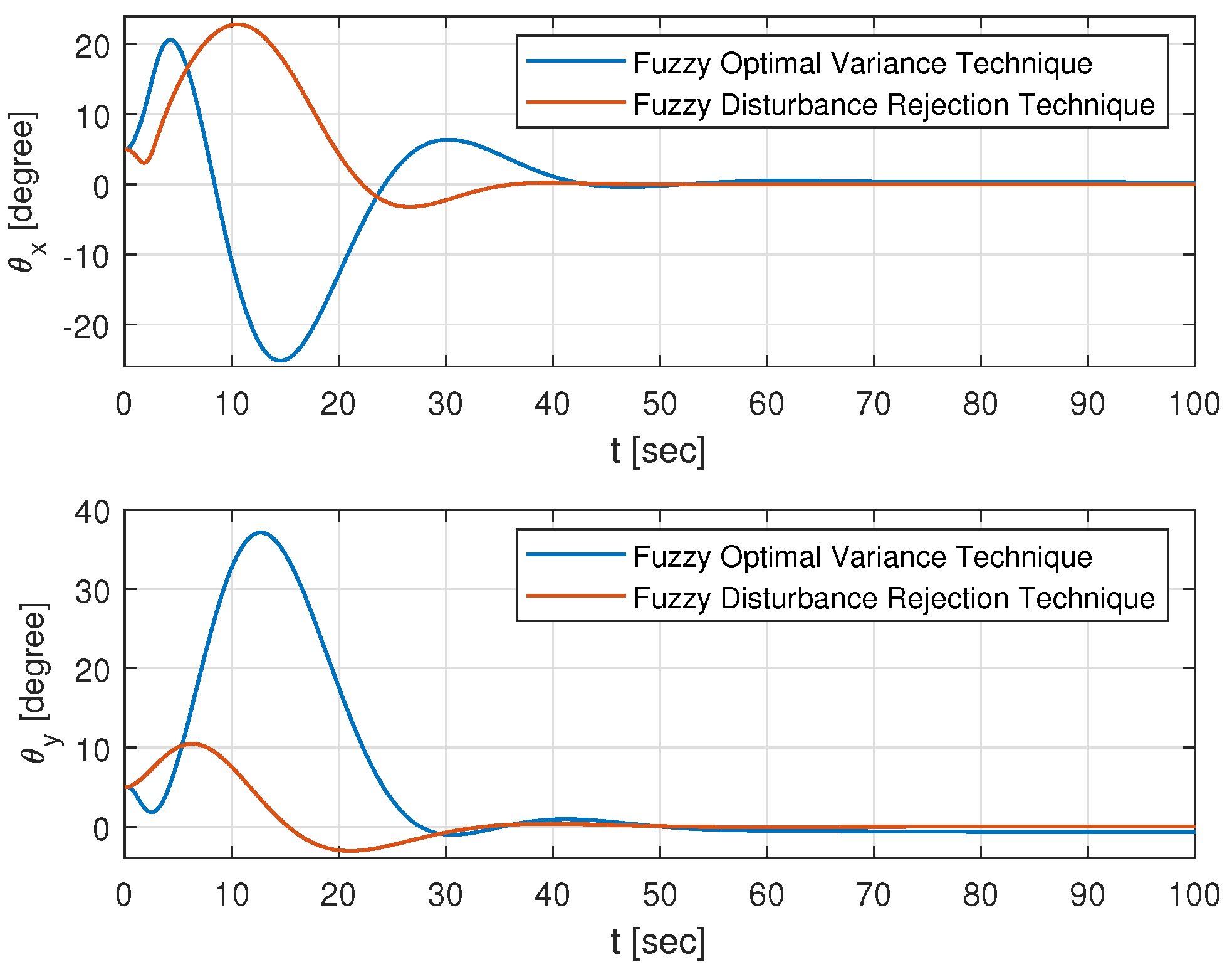
To compare the performance of the proposed controller, we use a fuzzy controller with disturbance rejection properties and constraints on the amplitude of the actuator alone. For detailed proof and the published results, we refer the reader to [39]. The following Figure 23 and Figure 24 show the performance of the proposed controller versus the fuzzy controller proposed in [39]. From the numerical simulation, we conclude that the performance of the optimal variance controller is almost similar to the fuzzy controller with disturbance rejection properties. It is worth mentioning that the fuzzy optimal variance controller is more advantageous since it includes constraints on the rate. The rate constraints are a significant parameter to consider during the design process of a spacecraft performing a bang-bang slew maneuver, as shown in this paper.
4. Conclusions
This paper presented a fuzzy optimal variance control technique applied to a flexible spacecraft equipped with multiple appendages during rest to rest slew maneuver. Because the maneuver performed by the spacecraft is bang-bang in nature, it tends to generate elastic deformation in the flexible appendages that can propagate throughout the entire spacecraft and degrade its performance. The spacecraft is equipped with actuators subject to amplitude and rate saturation. The fuzzy model used to develop the optimal variance controller is based on the Takagi-Sugeno fuzzy system with disturbances. The feedback gain is obtained by solving a set of linear matrix inequalities. The problem is formulated as an optimization problem and solved using the interior point method. The novelty of this paper is the application of the T-S fuzzy controller to a complex dynamical system with a large number of states, such as the flexible spacecraft. The numerical simulation and an evaluation of the closed-loop system versus a fuzzy controller with disturbance rejection properties and constraints on the amplitude of the actuator show that the proposed controller performance is satisfactory. It should be mentioned that there are some difficulties and challenges to overcome by using the proposed controller. For instance, obtaining a feasible solution is not evident, especially for a complex dynamic system with a large number of states. Further, if a viable solution is obtained, there is no guarantee that the controller’s performance will be adequate. Hence, further tuning is imperative. Unfortunately, there is no systematic way to tune the fuzzy controller except trial and error.
Funding
This research received no external funding.
Institutional Review Board Statement
Not applicable.
Informed Consent Statement
Not applicable.
Data Availability Statement
Not applicable.
Conflicts of Interest
The author declares no conflict of interest.
References
- Debelle, J. A Control Structure Based upon Process Models. J. A 1979, 20, 71–81. [Google Scholar]
- Fertik, H.A.; Ross, C.W. Direct Digital Control Algorithm with Anti-windup Feature. ISA Trans. 1967, 6, 317–328. [Google Scholar]
- Hanus, R. A New Technique for Preventing Control Windup. J. A 1980, 21, 15–20. [Google Scholar]
- Astrom, K.J.; Rundqwist, L. Integrator Windup and How to Avoid It. In Proceedings of the American Control Conference, Pittsburgh, PA, USA, 21–23 June 1989; Volume 2, pp. 1693–1698. [Google Scholar]
- Hanus, R. Antiwindup and Bumpless Transfer: A Survey. In Proceedings of the 12th IMACS World Congress, Paris, France, 18–22 July 1988; Volume 2, pp. 59–65. [Google Scholar]
- Morari, M. Some Control Problems in the Process Industries. In Essays on Control: Perspectives in the Theory and Its Applications; Birkhauser: Boston, MA, USA, 1993; pp. 55–77. [Google Scholar]
- Gilbert, E.G.; Kolmanovsky, I.; Tan, K.T. Discrete-time Reference Governors and the Nonlinear Control of Systems with State and Control Constraints. Int. J. Robust Nonlinear Control 1995, 5, 487–504. [Google Scholar] [CrossRef]
- Grimm, G.; Postlethwaite, I.; Teel, A.R.; Turner, M.C.; Zaccarian, L. Linear matrix inequalities for full and reduced order antiwindup synthesis. In Proceedings of the American Control Conference (Cat. No.01CH37148), Arlington, VA, USA, 25–27 June 2001; pp. 4134–4139. [Google Scholar] [CrossRef]
- Miyamoto, S.; Vinnicombe, G. Robust control of plants with saturation nonlinearity based on coprime factor representations. In Proceedings of the 35th IEEE Conference on Decision and Control, Kobe, Japan, 13 December 1996; Volume 3, pp. 2838–2840. [Google Scholar] [CrossRef]
- Mulder, E.F.; Kothare, M.V.; Morari, M. Multivariable anti-windup controller synthesis using iterative linear matrix inequalities. In Proceedings of the European Control Conference (ECC), Karlsruhe, Germany, 31 August–3 September 1999; pp. 3531–3536. [Google Scholar] [CrossRef]
- Shamma, J.S. Anti-windup via constrained regulation with observers. In Proceedings of the 1999 American Control Conference (Cat. No. 99CH36251), San Diego, CA, USA, 2–4 June 1999; Volume 4, pp. 2481–2485. [Google Scholar] [CrossRef]
- Teel, A.R. Anti-windup for exponentially unstable linear systems. Int. J. Robust Nonlinear Control 1999, 9, 701–716. [Google Scholar] [CrossRef]
- Teel, A.R.; Kapoor, N. The L2 anti-winup problem: Its definition and solution. In Proceedings of the European Control Conference (ECC), Brussels, Belgium, 1–7 July 1997; pp. 1897–1902. [Google Scholar]
- Zheng, A.; Kothare, M.V.; Morari, M. Anti-windup Design for Internal Model Control. Int. J. Control 1994, 60, 1015–1024. [Google Scholar] [CrossRef] [Green Version]
- Dornheim, M.A. Report Pinpoints Factors Leading to the YF-22 Crash. Aviat. Week Space Technol. 1992, 9, 53–54. [Google Scholar]
- Graettinger, T.J.; Krogh, B.H. Reference Signal Derivative Constraints for Guaranteed Tracking Performance. In Proceedings of the American Control Conference, Pittsburgh, PA, USA, 21–23 June 1989; pp. 2702–2707. [Google Scholar] [CrossRef]
- McNamee, J.; Pachter, M. The Construction of the Set of Stable States for Contrained Systems with Open-Loop Unstable Plants. In Proceedings of the 1998 American Control Conference ACC (IEEE Cat. No. 98CH36207), Philadelphia, PA, USA, 26 June 1998; pp. 3364–3368. [Google Scholar]
- Pachter, M.; Miller, R.B. Manual flight control with saturating actuators. IEEE Control Syst. Mag. 1998, 18, 10–20. [Google Scholar] [CrossRef]
- Goodwin, G.C.; Graebe, S.F.; Levin, W. Internal Model Control of Linear Systems with Saturating Actuators. In Proceedings of the European Control Conference, Groningen, The Netherlands, 28 June–1 July 1993; pp. 1072–1077. [Google Scholar]
- Seron, M.M.; Goodwin, G.C.; Graebe, S.F. Control system design issues for unstable linear systems with saturated inputs. In Proceedings of the IEE Proceedings-Control Theory and Applications; 1995; Volume 142, pp. 335–344. [Google Scholar] [CrossRef]
- Teel, A.R.; Kapoor, N. Uniting local and global controllers. In Proceedings of the European Control Conference (ECC), Brussels, Belgium, 1–7 July 1997; pp. 3868–3873. [Google Scholar] [CrossRef]
- Mamdani, E.H.; Assilian, S. An experiment in linguistic synthesis with a fuzzy logic controller. Int. J.-Man–Mach. Stud. 1975, 7, 1–13, ISSN 0020-7373. [Google Scholar] [CrossRef]
- Tanaka, K.; Sugeno, M. Stability analysis and design of fuzzy control systems. Fuzzy Sets Syst. 1992, 45, 135–156, ISSN 0165-0114. [Google Scholar] [CrossRef]
- Langari, G.; Tomizuka, M. Stability of fuzzy linguistic control systems. In Proceedings of the 29th IEEE Conference on Decision and Control, Honolulu, HI, USA, 5–7 December 1990; Volume 4, p. 2185. [Google Scholar] [CrossRef]
- Singh, S. Stability analysis of discrete fuzzy control systems. In Proceedings of the 1st IEEE International Conference Fuzzy Systems, San Diego, CA, USA, 8–12 March 1992; pp. 527–534. [Google Scholar]
- Feng, G. Controller synthesis of fuzzy dynamic systems based on piecewise lyapunov functions. IEEE Trans. Fuzzy Syst. 2003, 11, 605–612. [Google Scholar] [CrossRef]
- Tanaka, K.; Taniguchi, T.; Wang, H.O. Trajectory Control of an Articulated Vehicle with Triple Trailers. In Proceedings of the IEEE International Conference on Control Applications, Kohala Coast, HI, USA, 22–27 August 1999; Volume 2. [Google Scholar]
- Tanaka, K.; Ikeda, T.; Wang, H.O. Fuzzy regulators and fuzzy observers: Relaxed stability conditions and lmi-based designs. IEEE Trans. Fuzzy Syst. 1998, 6, 250–264. [Google Scholar] [CrossRef] [Green Version]
- Wang, H.O.; Tanaka, K.; Griffin, M. An approach to fuzzy control of nonlinear systems: Stability and design issues. IEEE Trans. Fuzzy Syst. 1996, 4, 14–23. [Google Scholar] [CrossRef]
- Sendi, C.; Ayoubi, M.A. Robust-Optimal Fuzzy Model-Based Control Of Flexible Spacecraft with Actuator Constraints. J. Dyn. Syst. Meas. Control 2015, 138, 091004. [Google Scholar] [CrossRef]
- Sendi, C.; Ayoubi, M.A. Robust Fuzzy Logic-Based Tracking Control of a Flexible Spacecraft with H∞ Performance Criteria. In Proceedings of the AIAA Space Conference and Exposition, San Diego, CA, USA, 10–12 September 2013. [Google Scholar] [CrossRef]
- Sendi, C. Attitude Stabilization during Retargeting Maneuver of Flexible Spacecraft Subject to Time Delay and Actuators Saturation. In Proceedings of the 2020 IEEE Aerospace Conference, Big Sky, MT, USA, 7–14 March 2020; pp. 1–10. [Google Scholar] [CrossRef]
- Meirovitch, L.; Kwak, K.M. Dynamics and control of spacecraft with retargeting flexible antennas. J. Guid. Control Dyn. 1990, 13, 241–248. [Google Scholar] [CrossRef]
- Meirovitch, L. Dynamics and Control of Structures; John Wiley & Sons, Inc.: Hoboken, NJ, USA, 1991; ISBN 978-0-471-62858-3. [Google Scholar]
- Meirovitch, L. Methods of Analytical Dynamics; Dover Publications, Inc.: Mineola, NY, USA, 2003. [Google Scholar]
- Swei, S.S.M.; Ayoubi, M.A. LMI-based fuzzy optimal variance control of airfoil model subject to input constraints. In Proceedings of the IEEE International Conference on Fuzzy Systems (FUZZ-IEEE), Naples, Italy, 9–12 July 2017; pp. 1–6. [Google Scholar] [CrossRef] [Green Version]
- Wang, H.O.; Tanaka, K. Parallel Distributed Compensation of Nonlinear Systems by Takagi-Sugeno Fuzzy Model. In Proceedings of the 1995 IEEE International Conference on Fuzzy Systems, Yokohama, Japan, 20–24 March 1995; Volume 2, pp. 531–538. [Google Scholar] [CrossRef]
- Lofberg, J. YALMIP: A toolbox for modeling and optimization in MATLAB. In Proceedings of the IEEE International Conference on Robotics and Automation (IEEE Cat. No.04CH37508), Taipei, Taiwan, 2–4 September 2004; pp. 284–289. [Google Scholar] [CrossRef]
- Ayoubi, M.A.; Sendi, C. Takagi-Sugeno Fuzzy Model-Based Control of Spacecraft with Flexible Appendage. J. Astronaut. Sci. 2014, 61, 40–59. [Google Scholar] [CrossRef]
Figure 1.
Model of the flexible spacecraft.

Figure 2.
Appendage time history.

Figure 3.
Fuzzy membership function.

Figure 4.
Position of the center of mass.

Figure 5.
Angular position of the spacecraft.

Figure 6.
Appendage 1 displacement.

Figure 7.
Appendage 2 displacement.

Figure 8.
Position of the center of mass.

Figure 9.
Angular position of the spacecraft.

Figure 10.
Displacement of appendage 1.

Figure 11.
Displacement of appendage 2.

Figure 12.
Actuator forces and moments.

Figure 13.
Actuator forces on the appendages.

Figure 14.
Position of the center of mass of the spacecraft with reduced settling time.

Figure 15.
Angular position of the spacecraft with reduced settling time.

Figure 16.
Displacement of appendage 1 with reduced settling time.

Figure 17.
Actuator with larger forces.

Figure 18.
Actuator with a larger torque.

Figure 19.
Position of the center of mass.

Figure 20.
Angular position of the spacecraft.

Figure 21.
Displacement of appendage 1.

Figure 22.
Displacement of appendage 2.

Figure 23.
Position of the center of mass of the spacecraft.

Figure 24.
Angular position of the spacecraft.

Table 1.
Parameter of the flexible spacecraft.
| Parameters | Values |
|---|---|
| [0.7341, 1.0185, 0.9992, 1, 1] | |
| [0.3750, 0.9388, 1.5800, 2.1990, 2.8274] | |
| m | |
| m | |
| kg | |
| kg | |
| kg·m2 | |
| kg·m2 | |
Publisher’s Note: MDPI stays neutral with regard to jurisdictional claims in published maps and institutional affiliations. |
© 2022 by the author. Licensee MDPI, Basel, Switzerland. This article is an open access article distributed under the terms and conditions of the Creative Commons Attribution (CC BY) license (https://creativecommons.org/licenses/by/4.0/).
Share and Cite
MDPI and ACS Style
Sendi, C. Attitude Control of a Flexible Spacecraft via Fuzzy Optimal Variance Technique. Mathematics 2022, 10, 179. https://doi.org/10.3390/math10020179
AMA Style
Sendi C. Attitude Control of a Flexible Spacecraft via Fuzzy Optimal Variance Technique. Mathematics. 2022; 10(2):179. https://doi.org/10.3390/math10020179
Chicago/Turabian StyleSendi, Chokri. 2022. "Attitude Control of a Flexible Spacecraft via Fuzzy Optimal Variance Technique" Mathematics 10, no. 2: 179. https://doi.org/10.3390/math10020179
Note that from the first issue of 2016, this journal uses article numbers instead of page numbers. See further details here.