
Model Fusion from Unauthorized Clients in Federated Learning


Abstract
:1. Introduction
- We propose FedUmf, which enables clients that are not authorized to upload model in each round to compute model updates and fuse the update later when they receive the upload authorization.
- We rigorously prove the convergence behavior of FedUmf for both strongly convex and non-convex loss functions. The results show that FedUmf strictly dominates the standard FedAvg.
- We selected the standard MNIST and CIFAR10 data set in the experiment, and carried out standardized preprocessing. Extensive experiments were conducted on two common data distributions (both independent and identically distributed (IID) and non-IID data distributions).
- We combine FedUmf with the state-of-art algorithm to show good test accuracy and the fastest convergence speed.
2. Related Works
3. The FedUmf Algorithm
3.1. The FL Model and FedAvg
3.2. FedUmf Algorithm Description
| Algorithm 1: FedUmf |
Initialize the weight ; Initialize the gradient ; ;  |
4. Analysis of Convergence
4.1. Strongly Convex Loss Function
- (1).
- For client , we have
- (2).
- For client , we have
- (3).
- For the other client , we have
4.2. Non-Convex Loss Function
5. Experiments
5.1. Experimental Setup
5.1.1. Models and Datasets
5.1.2. Hyperparameters
5.1.3. Criteria
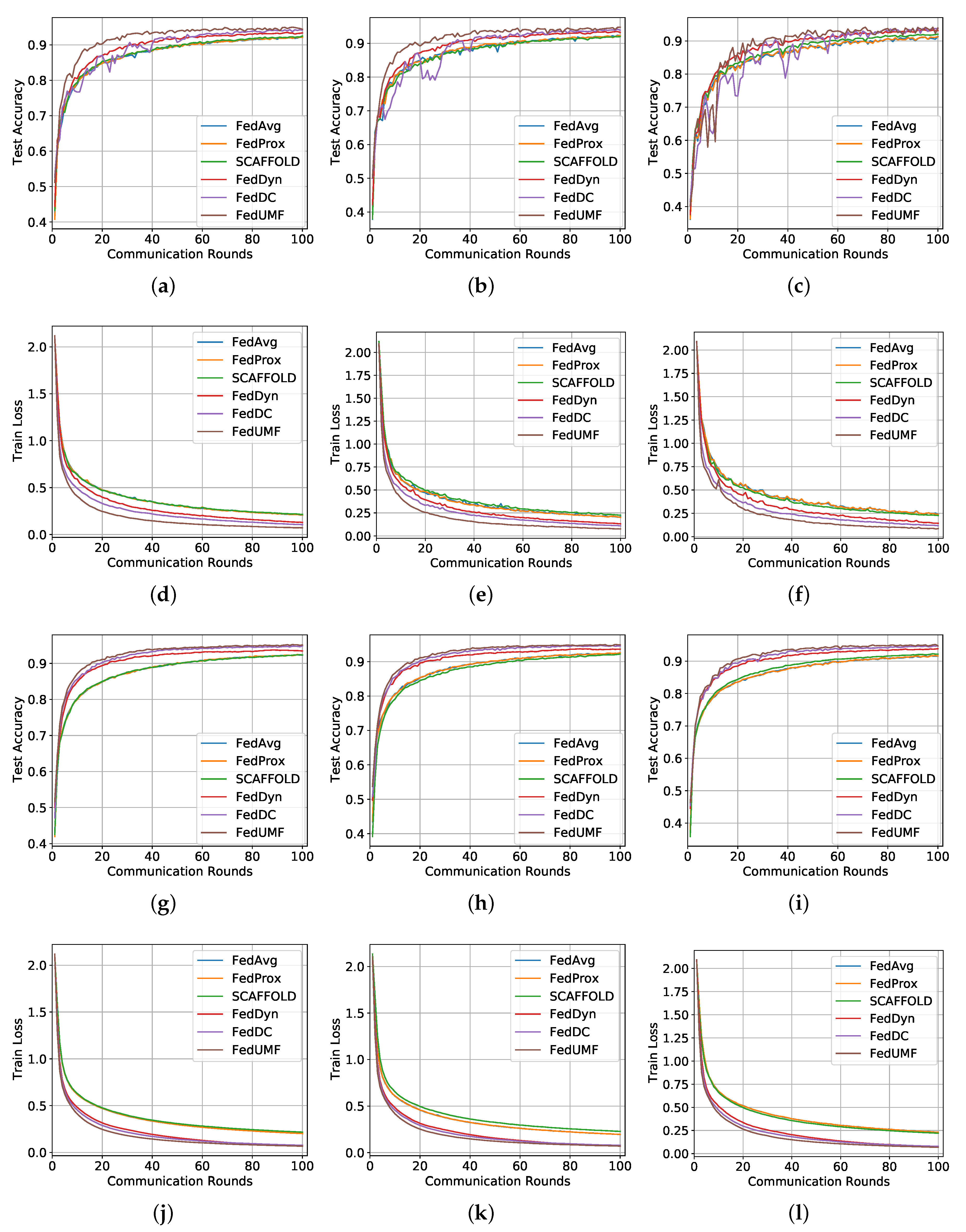
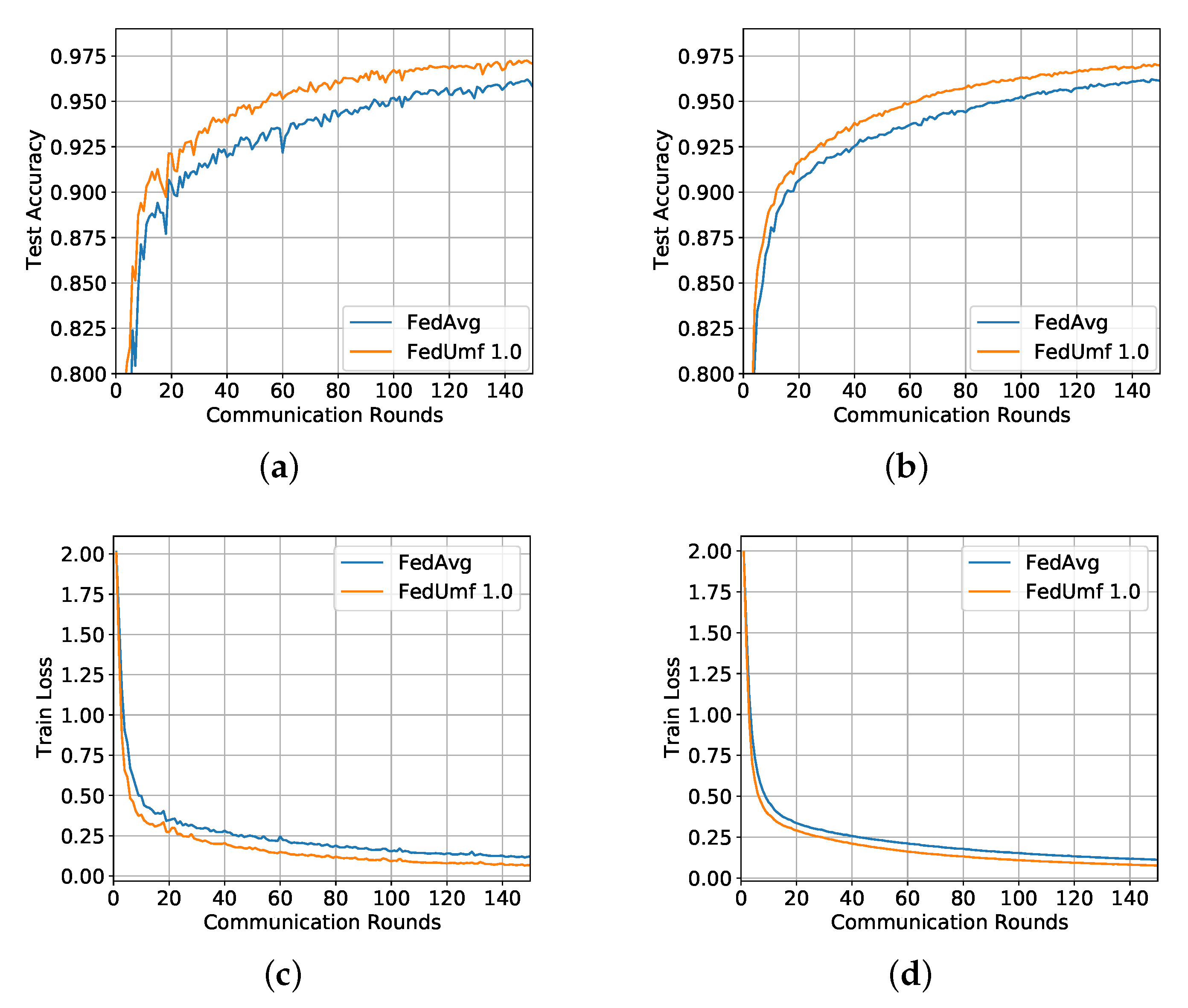
5.2. MNIST Results
5.2.1. IID Setting
5.2.2. Non-IID Setting
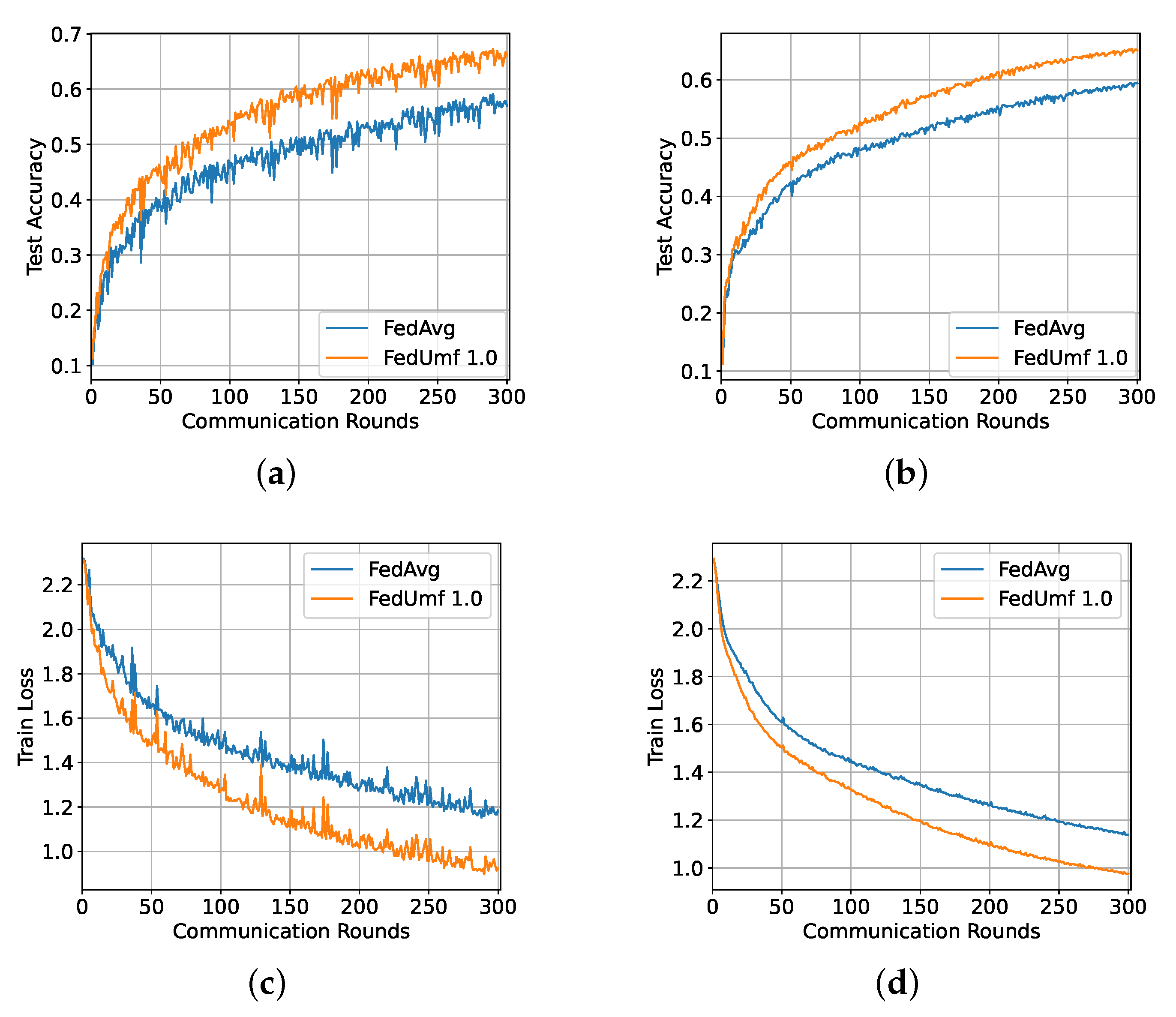
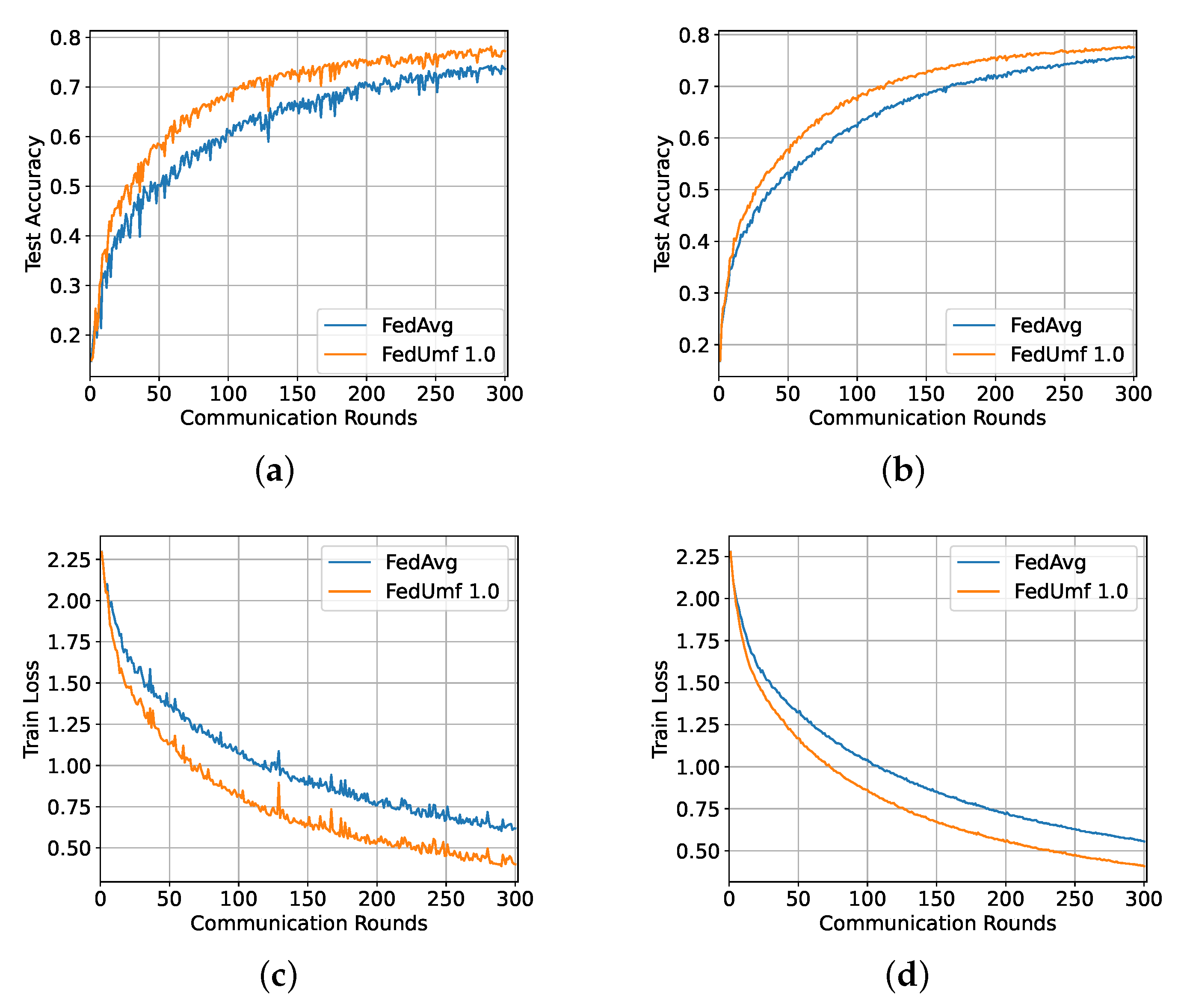
5.3. CIFAR10 Result
5.3.1. IID Setting
5.3.2. Non-IID Partition
6. Conclusions
Author Contributions
Funding
Data Availability Statement
Conflicts of Interest
Appendix A. Additional Experiments

| Methods | FedAvg | FedProx | SCAFFOLD | FedDyn | FedDC | FedUmf |
|---|---|---|---|---|---|---|
| Setting | 100 clients 15% participation | |||||
| MNIST-iid | 96.90 | 96.90 | 96.99 | 97.779 | 98.13 | 98.25 |
| MNIST-unbalance | 97.06 | 97.01 | 96.87 | 97.66 | 98.09 | 98.20 |
| MNIST-noniid | 96.45 | 96.44 | 96.85 | 97.56 | 98.09 | 98.21 |
| EMNIST-iid | 92.22 | 92.12 | 92.48 | 93.51 | 94.30 | 94.98 |
| EMNIST-unbalance | 92.41 | 92.31 | 92.01 | 93.48 | 94.15 | 94.78 |
| EMNIST-noniid | 91.36 | 91.26 | 92.06 | 93.36 | 94.13 | 94.16 |
| CIFAR10-iid | 74.12 | 74.24 | 74.1 | 81.90 | 81.89 | 82.90 |
| CIFAR10-unbalance | 74.14 | 74.25 | 72.30 | 81.77 | 81.92 | 82.45 |
| CIFAR10-noniid | 73.72 | 73.79 | 73.55 | 78.83 | 78.17 | 81.35 |
| CIFAR100-iid | 36.6 | 36.54 | 36.04 | 50.68 | 52.05 | 53.29 |
| CIFAR100-unbalance | 38.7 | 38.67 | 34.76 | 51.07 | 52.01 | 53.58 |
| CIFAR100-noniid | 35.92 | 36.15 | 35.88 | 43.08 | 43.43 | 51.11 |
| Setting | 100 clients 65% participation | |||||
| MNIST-iid | 96.98 | 96.96 | 97.06 | 98.01 | 98.34 | 98.40 |
| MNIST-unbalance | 97.20 | 97.20 | 96.88 | 97.90 | 98.33 | 98.34 |
| MNIST-noniid | 96.56 | 96.56 | 96.88 | 97.90 | 98.30 | 98.33 |
| EMNIST-iid | 92.35 | 92.46 | 92.45 | 93.75 | 94.86 | 95.25 |
| EMNIST-unbalance | 92.53 | 92.58 | 92.25 | 93.75 | 94.71 | 94.98 |
| EMNIST-noniid | 91.65 | 91.71 | 92.27 | 93.83 | 94.65 | 95.13 |
| CIFAR10-iid | 79.86 | 80.20 | 83.13 | 82.62 | 83.64 | 84.39 |
| CIFAR10-unbalance | 80.21 | 80.30 | 82.81 | 82.90 | 83.40 | 84.54 |
| CIFAR10-noniid | 78.34 | 78.41 | 81.73 | 81.92 | 82.42 | 82.89 |
| CIFAR100-iid | 36.69 | 36.42 | 47.30 | 47.10 | 52.53 | 54.48 |
| CIFAR100-unbalance | 38.12 | 38.10 | 48.94 | 47.22 | 52.92 | 54.23 |
| CIFAR100-noniid | 37.79 | 38.02 | 46.75 | 47.42 | 51.42 | 54.43 |
| Model | 100 Clients 15% Participation | 100 Clients 65% Participation | ||||||||||
|---|---|---|---|---|---|---|---|---|---|---|---|---|
| iid | unbalance | noniid | iid | unbalance | noniid | |||||||
| com R□ | Speed ⇑ | com R□ | Speed⇑ | com R□ | Speed ⇑ | com R□ | Speed ⇑ | com R□ | Speed⇑ | com R□ | Speed ⇑ | |
| MNIST, Target accuracy 95% | ||||||||||||
| FedAvg | 40 | - | 34 | - | 52 | - | 36 | - | 32 | - | 59 | - |
| FedProx | 40 | 1.00× | 35 | 0.97× | 52 | 1.00× | 36 | 1.00× | 31 | 1.03× | 49 | 1.20× |
| SCAFFOLD | 39 | 1.03× | 42 | 0.81× | 43 | 1.21× | 35 | 1.03× | 38 | 0.84× | 39 | 1.51× |
| FedDyn | 25 | 1.60× | 25 | 1.36× | 31 | 1.68× | 11 | 3.27× | 16 | 2.00× | 16 | 3.69× |
| FedDC | 22 | 1.82× | 28 | 1.21× | 24 | 2.17× | 25 | 1.44× | 14 | 2.29× | 14 | 4.21× |
| FedUmf | 11 | 3.64× | 12 | 2.83× | 14 | 3.71× | 10 | 3.60× | 10 | 3.20× | 12 | 4.92× |
| EMNIST, Target accuracy 91% | ||||||||||||
| FedAvg | 67 | - | 68 | - | 87 | - | 62 | - | 57 | - | 83 | - |
| FedProx | 69 | 0.97× | 68 | 1.00× | 92 | 0.95× | 62 | 1.00× | 58 | 0.98× | 81 | 1.02× |
| SCAFFOLD | 64 | 1.05× | 72 | 0.94× | 74 | 1.18× | 62 | 1.00× | 68 | 0.84× | 67 | 1.24× |
| FedDyn | 39 | 1.72× | 39 | 1.74× | 55 | 1.58× | 29 | 2.14× | 28 | 2.04× | 36 | 2.31× |
| FedDC | 40 | 1.68× | 34 | 2.00× | 46 | 1.89× | 23 | 2.70× | 23 | 2.48× | 28 | 2.96× |
| FedUmf | 21 | 3.19× | 24 | 2.83× | 33 | 2.64× | 19 | 3.26× | 19 | 3.00× | 21 | 3.95× |
| CIFAR10, Target accuracy 70% | ||||||||||||
| FedAvg | 197 | - | 180 | - | 225 | - | 50 | - | 50 | - | 74 | - |
| FedProx | 201 | 0.98× | 179 | 1.01× | 225 | 1.00× | 50 | 1.00× | 50 | 1.00× | 74 | 1.00× |
| SCAFFOLD | 213 | 0.92× | 236 | 0.76× | 225 | 1.0× | 37 | 1.35× | 51 | 0.98× | 69 | 1.07× |
| FedDyn | 70 | 2.81× | 71 | 2.54× | 125 | 1.8× | 42 | 1.19× | 50 | 1.00× | 69 | 1.07× |
| FedDC | 69 | 2.86× | 72 | 2.50× | 125 | 1.80× | 31 | 1.61× | 50 | 1.00× | 50 | 1.48× |
| FedUmf | 50 | 3.94× | 51 | 3.53× | 62 | 3.63× | 28 | 1.79× | 40 | 1.25× | 46 | 1.61× |
| CIFAR100, Target accuracy 35% | ||||||||||||
| FedAvg | 198 | - | 165 | - | 203 | - | 213 | - | 149 | - | 175 | - |
| FedProx | 198 | 1.00× | 165 | 1.00× | 203 | 1.00× | 213 | 1.0× | 148 | 1.01× | 176 | 0.99× |
| SCAFFOLD | 207 | 0.96× | 220 | 0.75× | 205 | 0.99× | 69 | 3.09× | 70 | 2.13× | 73 | 2.40× |
| FedDyn | 75 | 2.64× | 76 | 2.17× | 109 | 1.86× | 100 | 2.13× | 99 | 1.51× | 103 | 1.70× |
| FedDC | 74 | 2.68× | 72 | 2.29× | 105 | 1.93× | 77 | 2.77× | 73 | 2.04× | 78 | 2.24× |
| FedUmf | 63 | 3.14× | 65 | 2.54× | 70 | 2.90× | 40 | 5.33× | 49 | 3.04× | 50 | 3.50× |


References
- Bonawitz, K.; Eichner, H.; Grieskamp, W.; Huba, D.; Ingerman, A.; Ivanov, V.; Kiddon, C.; Konečný, J.; Mazzocchi, S.; McMahan, B.; et al. Towards federated learning at Scale: System design. In Proceedings of the 2nd SysML Conference, Stanford, CA, USA, 31 March–2 April 2019; pp. 1–15. [Google Scholar]
- McMahan, B.; Moore, E.; Ramage, D.; Hampson, S.; Arcas, B.A. Communication-Efficient Learning of Deep Networks from Decentralized Data. In Proceedings of the 20th International Conference on Artificial Intelligence and Statistics (AISTATS), Lauderdale, FL, USA, 20–22 April 2017; pp. 1273–1282. [Google Scholar]
- Konecný, J.; McMahan, H.B.; Yu, F.X.; Richtárik, P.; Suresh, A.T.; Bacon, D. Federated Learning: Strategies for Improving Communication Efficiency. In Proceedings of the NIPS Workshop on Private Multi-Party Machine Learning, Barcelona, Spain, 9 December 2016. [Google Scholar]
- Robbins, H.; Monro, S. A Stochastic Approximation Method. Ann. Math. Stat. 1951, 22, 400–407. [Google Scholar] [CrossRef]
- Kairouz, P.; McMahan, H.B.; Avent, B.; Bellet, A.; Bennis, M.; Bhagoji, A.N.; Zhao, S. Advances and open problems in federated learning. arXiv 2019, arXiv:1912.04977. [Google Scholar]
- Li, T.; Sahu, A.K.; Talwalkar, A.; Smith, V. Federated learning: Challenges, methods, and future directions. IEEE Signal Process. Mag. 2020, 37, 50–60. [Google Scholar] [CrossRef]
- Imteaj, A.; Thakker, U.; Wang, S.; Li, J.; Amini, M.H. A Survey on Federated Learning for Resource-Constrained IoT Devices. IEEE Internet Things J. 2022, 9, 1–24. [Google Scholar] [CrossRef]
- Bernstein, J.; Wang, Y.; Azizzadenesheli, K.; Anandkumar, A. signSGD: Compressed optimisation for non-convex problems. arXiv 2018, arXiv:1802.04434. [Google Scholar]
- Wen, W.; Xu, C.; Yan, F.; Wu, C.; Wang, Y.; Chen, Y.; Li, H. TernGrad: Ternary Gradients to Reduce Communication in Distributed Deep Learning. In Proceedings of the Advances in Neural Information Processing Systems, Long Beach, CA, USA, 4–9 December 2017; pp. 1509–1519. [Google Scholar]
- Woodworth, B.E.; Wang, J.; Smith, A.; McMahan, B.; Srebro, N. Graph oracle models, lower bounds, and gaps for parallel stochastic optimization. In Proceedings of the Advances in Neural Information Processing Systems, Montréal, QC, Canada, 3–8 December 2018; pp. 8496–8506. [Google Scholar]
- Zhou, F.; Cong, G. On the Convergence Properties of a K-step Averaging Stochastic Gradient Descent Algorithm for Nonconvex Optimization. In Proceedings of the Twenty-Seventh International Joint Conference on Artificial Intelligence, Stockholm, Sweden, 13–19 July 2018; pp. 3219–3227. [Google Scholar]
- Sattler, F.; Wiedemann, S.; Müller, K.; Samek, W. Robust and Communication-Efficient Federated Learning From Non-i.i.d. Data. IEEE Trans. Neural Netw. Learn. Syst. 2019, 31, 3400–3413. [Google Scholar] [CrossRef] [Green Version]
- Karimireddy, S.P.; Rebjock, Q.; Stich, S.U.; Jaggi, M. Error Feedback Fixes SignSGD and other Gradient Compression Schemes. arXiv 2019, arXiv:1901.09847. [Google Scholar]
- Reisizadeh, A.; Mokhtari, A.; Hassani, H.; Pedarsani, R. An Exact Quantized Decentralized Gradient Descent Algorithm. IEEE Trans. Signal Process. 2019, 67, 4934–4947. [Google Scholar] [CrossRef] [Green Version]
- Yuan, J.; Xu, M.; Ma, X.; Zhou, A.; Liu, X.; Wang, S. Hierarchical Federated Learning through LAN-WAN Orchestration. arXiv 2020, arXiv:2010.11612. [Google Scholar]
- Dai, X.; Yan, X.; Zhou, K.; Yang, H.; Ng, K.K.W.; Cheng, J.; Ling Fan, Y. Hyper-Sphere Quantization: Communication-Efficient SGD for Federated Learning. arXiv 2019, arXiv:1911.04655. [Google Scholar]
- Konecný, J. Stochastic, Distributed and Federated Optimization for Machine Learning. arXiv 2017, arXiv:1707.01155. [Google Scholar]
- Yu, Y.; Wu, J.; Huang, L. Double Quantization for Communication-Efficient Distributed Optimization. In Proceedings of the Advances in Neural Information Processing Systems, Vancouver, BC, Canada, 8–14 December 2019; pp. 4440–4451. [Google Scholar]
- Sahu, A.K.; Li, T.; Sanjabi, M.; Zaheer, M.; Talwalkar, A.; Smith, V. On the Convergence of Federated Optimization in Heterogeneous Networks. arXiv 2018, arXiv:1812.06127. [Google Scholar]
- Alistarh, D.; Grubic, D.; Li, J.; Tomioka, R.; Vojnovic, M. QSGD: Communication-Efficient SGD via Gradient Quantization and Encoding. In Proceedings of the Advances in Neural Information Processing Systems, Long Beach, CA, USA, 4–9 December 2017; pp. 1709–1720. [Google Scholar]
- Jiang, P.; Agrawal, G. A Linear Speedup Analysis of Distributed Deep Learning with Sparse and Quantized Communication. In Proceedings of the Advances in Neural Information Processing Systems, Montréal, QC, Canada, 3–8 December 2018; pp. 2525–2536. [Google Scholar]
- Lu, X.; Liao, Y.; Liu, C.; Lio, P.; Hui, P. Heterogeneous Model Fusion Federated Learning Mechanism Based on Model Mapping. IEEE Internet Things J. 2022, 9, 6058–6068. [Google Scholar] [CrossRef]
- Yu, L.; Albelaihi, R.; Sun, X.; Ansari, N.; Devetsikiotis, M. Jointly Optimizing Client Selection and Resource Management in Wireless Federated Learning for Internet of Things. IEEE Internet Things J. 2022, 9, 4385–4395. [Google Scholar] [CrossRef]
- Wu, W.; He, L.; Lin, W.; Mao, R.; Maple, C.; Jarvis, S.A. SAFA: A Semi-Asynchronous Protocol for Fast Federated Learning with Low Overhead. IEEE Trans. Comput. 2020, 70, 655–668. [Google Scholar] [CrossRef]
- Zhang, T.; Song, A.; Dong, X.; Shen, Y.; Ma, J. Privacy-Preserving Asynchronous Grouped Federated Learning for IoT. IEEE Internet Things J. 2022, 9, 5511–5523. [Google Scholar] [CrossRef]
- Zhang, W.; Gupta, S.; Lian, X.; Liu, J. Staleness-aware Async-SGD for Distributed Deep Learning. arXiv 2015, arXiv:1511.05950. [Google Scholar]
- Xie, C.; Koyejo, S.; Gupta, I. Asynchronous Federated Optimization. arXiv 2019, arXiv:1903.03934. [Google Scholar]
- Chen, Y.; Nin, Y.; Slawski, M.; Rangwala, H. Asynchronous Online Federated Learning for Edge Devices. arXiv 2019, arXiv:1911.02134. [Google Scholar]
- Zheng, S.; Meng, Q.; Wang, T.; Chen, W.; Yu, N.; Ma, Z.M.; Liu, T.Y. Asynchronous Stochastic Gradient Descent with Delay Compensation. In Proceedings of the Machine Learning Research; PMLR International Convention Centre: Sydney, Australia, 2017; Volume 70, pp. 4120–4129. [Google Scholar]
- Reisizadeh, A.; Mokhtari, A.; Hassani, H.; Jadbabaie, A.; Pedarsani, R. FedPAQ: A communication-efficient federated learning method with periodic averaging and quantization. In Proceedings of the 23rd International Conference on Artificial Intelligence and Statistics (AISTATS), Palermo, Italy, 26–28 August 2020. [Google Scholar]
- Stich, S.U. Local SGD Converges Fast and Communicates Little. In Proceedings of the International Conference on Learning Representations, Vancouver, BC, Canada, 30 March–3 May 2018. [Google Scholar]
- Wang, J.; Joshi, G. Cooperative SGD: A unified framework for the design and analysis of communication-efficient SGD algorithms. arXiv 2018, arXiv:1808.07576. [Google Scholar]
- Yu, H.; Yang, S.; Zhu, S. Parallel restarted SGD for non-convex optimization with faster convergence and less communication. arXiv 2018, arXiv:1807.06629. [Google Scholar]
- He, K.; Zhang, X.; Ren, S.; Sun, J. Deep Residual Learning for Image Recognition. In Proceedings of the CVPR, Las Vegas, NV, USA, 27–30 June 2016; pp. 770–778. [Google Scholar]
- Karimireddy, S.P.; Kale, S.; Mohri, M.; Reddi, S.J.; Stich, S.U.; Suresh, A.T. SCAFFOLD: Stochastic controlled averaging for on-device federated learning. arXiv 2019, arXiv:1910.06378. [Google Scholar]
- Acar, D.A.E.; Zhao, Y.; Matas, R.; Mattina, M.; Whatmough, P.; Saligrama, V. Federated Learning Based on Dynamic Regularization. In Proceedings of the International Conference on Learning Representations (ICLR), Vienna, Austria, 3–7 May 2021. [Google Scholar]
- Gao, L.; Fu, H.; Li, L.; Chen, Y.; Xu, M.; Xu, C.Z. FedDC: Federated Learning with Non-IID Data via Local Drift Decoupling and Correction. In Proceedings of the IEEE Conference on Computer Vision and Pattern Recognition (CVPR), New Orleans, LA, USA, 19–24 June 2022. [Google Scholar]
- Lecun, Y.; Bottou, L.; Bengio, Y.; Haffner, P. Gradient-based learning applied to document recognition. Proc. IEEE 1998, 86, 2278–2324. [Google Scholar] [CrossRef]
- Cohen, G.; Afshar, S.; Tapson, J.; van Schaik, A. EMNIST: Extending MNIST to handwritten letters. In Proceedings of the 2017 International Joint Conference on Neural Networks (IJCNN), Anchorage, AK, USA, 14–19 May 2017; pp. 2921–2926. [Google Scholar] [CrossRef]
- Krizhevsky, A. Learning Multiple Layers of Features from Tiny Images. Master’s Thesis, University of Tronto, Toronto, ON, Canada, 2009. [Google Scholar]
- Lin, T.; Karimireddy, S.P.; Stich, S.U.; Jaggi, M. Quasi-global momentum: Accelerating decentralized deep learning on heterogeneous data. arXiv 2021, arXiv:2102.04761. [Google Scholar]


| Parameters, | Schemes | Accuracy | |||||
|---|---|---|---|---|---|---|---|
| 92% | 93% | 94% | 95% | 96% | 97% | ||
| FedAvg | 23 | 34 | 48 | 69 | 103 | * | |
| FedUmf | 14 | 21 | 28 | 39 | 55 | 99 | |
| FedAvg | 23 | 35 | 46 | 70 | 101 | * | |
| FedUmf | 17 | 24 | 32 | 47 | 66 | 110 | |
| FedAvg | 6 | 9 | 11 | 15 | 23 | 38 | |
| FedUmf | 5 | 6 | 7 | 10 | 15 | 25 | |
| FedAvg | 4 | 5 | 6 | 11 | 15 | 46 | |
| FedUmf | 4 | 5 | 6 | 9 | 15 | 29 | |
| Parameters, | Schemes | Accuracy | |||||
|---|---|---|---|---|---|---|---|
| 91% | 92% | 93% | 94% | 95% | 96% | ||
| FedAvg | 24 | 34 | 44 | 71 | 92 | 141 | |
| FedUmf | 12 | 18 | 29 | 34 | 54 | 69 | |
| FedAvg | 22 | 33 | 44 | 64 | 92 | 135 | |
| FedUmf | 15 | 23 | 32 | 44 | 62 | 87 | |
| FedAvg | 7 | 8 | 11 | 14 | 22 | 31 | |
| FedUmf | 5 | 7 | 8 | 10 | 11 | 23 | |
| FedAvg | 7 | 8 | 11 | 14 | 19 | 26 | |
| FedUmf | 5 | 6 | 8 | 10 | 14 | 21 | |
| Parameters, | Schemes | Accuracy | ||||||
|---|---|---|---|---|---|---|---|---|
| 30% | 40% | 50% | 55% | 60% | 65% | 70% | ||
| FedAvg | 6 | 25 | 82 | 130 | 207 | * | * | |
| FedUmf | 4 | 15 | 45 | 66 | 103 | 165 | 288 | |
| FedAvg | 4 | 25 | 78 | 128 | 200 | * | * | |
| FedUmf | 3 | 17 | 52 | 85 | 129 | 206 | * | |
| FedAvg | 4 | 11 | 33 | 53 | 76 | 108 | 157 | |
| FedUmf | 4 | 8 | 21 | 31 | 45 | 64 | 90 | |
| FedAvg | 3 | 10 | 30 | 46 | 67 | 97 | 140 | |
| FedUmf | 3 | 9 | 22 | 34 | 49 | 70 | 101 | |
| Parameters, | Schemes | Accuracy | |||||
|---|---|---|---|---|---|---|---|
| 45% | 50% | 55% | 60% | 65% | 70% | ||
| FedAvg | 74 | 129 | 224 | * | * | * | |
| FedUmf | 43 | 65 | 103 | 146 | 230 | * | |
| FedAvg | 69 | 124 | 194 | * | * | * | |
| FedUmf | 44 | 78 | 122 | 183 | 290 | * | |
| FedAvg | 31 | 43 | 65 | 95 | 129 | 191 | |
| FedUmf | 17 | 25 | 39 | 54 | 74 | 108 | |
| FedAvg | 24 | 37 | 57 | 82 | 116 | 167 | |
| FedUmf | 18 | 26 | 40 | 57 | 81 | 116 | |
Publisher’s Note: MDPI stays neutral with regard to jurisdictional claims in published maps and institutional affiliations. |
© 2022 by the authors. Licensee MDPI, Basel, Switzerland. This article is an open access article distributed under the terms and conditions of the Creative Commons Attribution (CC BY) license (https://creativecommons.org/licenses/by/4.0/).
Share and Cite
Li, B.; Chen, S.; Yu, K. Model Fusion from Unauthorized Clients in Federated Learning. Mathematics 2022, 10, 3751. https://doi.org/10.3390/math10203751
Li B, Chen S, Yu K. Model Fusion from Unauthorized Clients in Federated Learning. Mathematics. 2022; 10(20):3751. https://doi.org/10.3390/math10203751
Chicago/Turabian StyleLi, Boyuan, Shengbo Chen, and Keping Yu. 2022. "Model Fusion from Unauthorized Clients in Federated Learning" Mathematics 10, no. 20: 3751. https://doi.org/10.3390/math10203751