1. Introduction
Graph matching has been applied in a variety of fields, including biological applications [
1], remote sensing image recognition [
2], and image retrieval [
3]. The key to graph matching is to find correspondences between image visual features using particular algorithms. Graph matching is typically viewed as a quadratic assignment problem (QAP) [
4], and since the quadratic objective function is also non-convex, obtaining the global optimal value is challenging [
5]. Various approximation algorithms have been developed to settle them under relatively relaxed conditions. Ref. [
6] proposed a matching approach based on linear programming. In [
7], semidefinite programming was used to solve such a problem, and [
8] adopted a similar strategy. However, these algorithms are locally optimal in the discrete domain, and discretization can cause extra errors. There are other methods based on tree search that focus on the suboptimality; for instance, Sanfeliu improved the previous method by considering the joint probability of points and edges in [
9]. In [
10], it is shown that random walk-based models greatly enhance the graph topological features. A. Robles-Kelly [
11] introduced a novel algorithm based on the relationship between the adjacent matrix of the two graphs and their stationary distribution.
Matching-based techniques have been adopted in a variety of study fields. Early classification based on sparse representation (SRC) [
12] is not satisfactory in the treatment of occlusion. With the development of multiview non-negative matrix factorization (NMF) methods [
13], the local geometry is preserved while global representation under a global alignment strategy is obtained. However, these methods are still affected by various noises and cannot highlight the target characteristics. In [
14], Ou et al. proposed a method that used adaptively estimated occlusion information and robustly selected features to improve the performance of facial recognition. The K-nearest neighbor (KNN) is also a non-parametric classifier that is widely used in pattern recognition. However, the performance of KNN-based classification is severely affected by the sensitivity of the neighbourhood size, especially when the sample size is small and there are outliers. Refs. [
15,
16] improve this problem by weighting and averaging, and have a robust and effective classification performance.
In recent years, high-order graph matching algorithms have put a large amount of attention on the better fusion of structural similarities in order to improve the matching accuracy. Zass and Shashua [
17] proposed a probabilistic setting-based hypergraph matching approach that uses an iterative successive projection process to find the global optimal solution. Lee et al. [
18] expanded the reweighted random walk approach to hypergraph matching and probabilistically reinterpreted the idea of random walk on hypergraphs. However, these matching algorithms employ Euclidean distance to generate an affinity matrix, and each feature attribute is regarded as being independent from the others. Traditional methods lack a specific metric for feature description, their performance on different types of data is highly variable, and their overall accuracy is low. In this paper, we present an improved hypergraph matching algorithm on the basis of the metric learning theory. By learning the training dataset, it obtains a Mahalanobis matrix that is used to consummate the affinity formulation. Since the Mahalanobis distance is a measure considering the correlation between feature descriptions as well as scaling relations, the assignment matrix obtained by this method would be closer to the ground truth; in fact, experiments show that our algorithm can improve the accuracy of their matching results. The main contributions of this manuscript are described as follows:
A novel approach for graph matching based on metric learning is proposed, in which, the correlation of different features is well considered so that it can perform better.
An information-theoretic metric learning (ITML) method was applied to solve the learning task under high-order graph matching.
The metric learning algorithm is proved by parallel computation, which greatly reduces the communication demands.
Compared with other state-of-the-art algorithms in experiments on test datasets, our proposed method can obtain more accurate results in an efficient way.
The rest of this article is structured as follows.
Section 2 begins with an overview of graph-matching-related work.
Section 3 presents the proposed model as well as the generic formula for graph matching.
Section 4 develops the MLGM approach for optimizing the suggested graph matching model.
Section 5 evaluates and analyzes the experimental results of the proposed method on synthetic and natural picture benchmarks. The final section is the conclusion.
2. Related Works
In the last few years, spectral methods have developed into one of the most representative algorithms in graph matching. The eigenvalues of a matrix do not change when its rows and columns are shuffled; thus, we can utilize this fact to find the adjacency matrix that has the same eigenvalues between similar pictures. Earlier, the spectral method was applied to perform feature matching [
19]. Ref. [
20] introduced a method incorporating the grey level information around the feature points to improve the matching accuracy. Leordeanu et al. [
8] proposed a matching algorithm by building an affinity matrix of the feature points that considered the effect of different weight functions in point matching. In another direction, the grouping method can also improve the effectiveness of matching. Egozi et al. [
21] proposed a probabilistic interpretation of spectral matching schemes and developed a unique probabilistic matching (PM) scheme that outperforms earlier methods. Feature matching carried out by means of alternating the embedding and matching of the adjacency spectrum was introduced in [
22], and, in [
23], a relaxation scheme with matching constraints was proposed. Duchenne et al. [
9] proposed a class algorithm that uses a tensor to represent similarities between higher-order features, and the graph can be matched after rank-one decomposition of the similarity tensor. This algorithm extends the spectral method to the hypergraph, and it has been further improved through research [
24]. The adjacency spectrum optimization of undirected weighted graphs [
25] and the approximation of the proximal matrix spectrum of undirected weighted graphs [
26] have been developed in recent years, and results have been gained in image processing applications.
The graph edit distance (GED), which represents the matching link between nodes and edges in two graphs, was utilized to solve graph matching. For example, Ref. [
27] proposed a self-organizing mapping algorithm to learn the distance, which makes the distance between similar images smaller, and this method was improved in [
28]. Serratosa proposed a method based on an adaptive learning paradigm, which was improved in [
29]. Andreas Fischer and Kaspar Riesen presented an algorithm [
30] combining Hausdorff matching with greedy allocation to improve the quadratic time approximation of GED.
Metric learning has been widely used in face recognition [
31,
32], image retrieval [
33], re-recognition [
34], and other fields. For traditional metric methods such as Euclidean distance, it is challenging to capture the structure of diverse data sets. In order to increase the performance of classification models, it is important to learn a specific measure for various data sets, which is the objective of metric learning. The algorithm for metric learning based on the Mahalanobis distance is still the primary focus of metric learning research at the present time. Bohne et al. [
35] proposed dividing the data and learning a metric for each cluster, and Wang et al. [
36] suggested learning a set of basis metrics and a set of weights for each sample.
3. Problem Statement
As a mathematical expression of a relationship, a graph model [
37] is composed of a node set and edge set. Finding the corresponding relationship between two graphs is the objective of graph matching. Generally, it seeks the relationship between nodes in graphs, and the specific node may be a pixel, a graph area, or a feature point. In the study of the graph matching and hypergraph matching algorithm, in order to express the relationship between graph features more comprehensively, the structure information of graph model is used to represent the problem in graph matching.
Figure 1 depicts a graph matching example diagram.
We now consider two sets of feature points
and
, which are extracted from graphs
A and
B, respectively. The number of points obtained in each graph is
m and
n, which can be the same or different. In the high-order graph matching algorithm [
9], what is different from the previous methods is that it matches a tuple of points instead of one to one or pair to pair, and
k is used here to represent the number of points in each tuple. High-order graph matching has a good robustness under unfavorable conditions such as noise deformation and the rotation of external points [
38], but it requires more space and time complexity. The third order can reflect the invariance of the similarity transformation in the field of computer vision, and, as the smallest higher-order topology, it can measure the subtle differences between high-order graphs. For convenience, only third-order graph matching is discussed in this paper, and it is straightforward to generalize to higher-order potentials.
The matching problem of the two graphs is to compute an optimal assignment relationship between points. Mathematically, this is the equivalent of finding an
assignment matrix
X. If the feature point
in
P matches
in
Q, then the corresponding
is equal to 1; otherwise, it is 0. In this paper, we assumed that each feature point in
P can match zero or more feature points in
Q, but each point in
Q can match only one point in
P. As a result, the set of assignment matrix
X can be denoted as
.
where
.
The universal second-order graph matching model can be used to solve
X as
where
M is an affinity tensor and represents the affinity relationship between point pairs (
) and (
).
is the sum of the affinity values of all of the matched tuples; the higher the value corresponds to, the more precise the matching result. Establishing the affinity tensor
M for two graphs
A and
B requires taking into account the similarity between pairs of nodes and pairs of edges.
f is the feature of each tuple, which is represented by Euclidean distance between points in second-order graph matching, and
is the parameter [
9].
However, the second-order graph matching model can only express paired relations, which are not resistant to scale changes and difficult to express higher-order feature information. Considering the high-order relation of feature points, we describe the similarity between feature point sets based on the relation between point tuples. Given two point sets
P and
Q, the affinity tensor can be expressed as
where
,
,
represent the point tuples in point set
P of graph
A,
,
,
represent the three potential point tuples to be matched in point set
Q of graph
B,
is a constant that controls the distribution of the intimacy tensor value, and
and
represent the vectors constructed from the feature information of point tuples in point set
P and
Q, respectively. There are numerous ways to represent feature information; for ease of calculation, we use the sine value of the inner angle of the triangle formed by point tuples.
Similar to model (
2), the high-order graph matching model can be formulated as
In (
5), only when point tuples (
) match (
) separately does
equal 1. This is an optimal solution problem; by finding the assignment matrix corresponding to the maximum value of
, the matching relation between tuples can be obtained. We can also write (
5) as (
6) by using the notation of tensor–vector multiplication:
where
represents the vector created by combining the
X columns,
stands for the symmetric matrix produced by tensor expansion, and
I,
J, and
K are the three dimensions of tensor
M.
In the traditional affinity measure, Function (
4), each feature is considered to be of the same importance. However, because these features may have different correlations with sample categories, their weights need to be reconsidered. In other words, a suitable distance or similarity measure based on the feature space of the sample should be used to measure the difference in the sample. Due to its two characteristics, decoupling and dimensionality independence, Mahalanobis distance [
39] is an excellent measurement function for image processing and computer vision. In this paper, we used the Mahalanobis distance function to measure the affinity of feature vectors and create the appropriate metric learning model.
4. Tensor Affinity Learning for Hyperorder Graph Matching
4.1. A Short Introduction to Metric Learning
The study of metric learning has significant theoretical implications. Metric learning is concerned with developing an accurate function model for an input feature vector and obtaining an accurate similarity measure by learning the model’s parameters. It can enhance the performance of the classifier by generating similarity relationships with high accuracy [
40]. However, how to accurately measure the similarity of samples affected by different external factors is overlooked. The simple normalization method is used to preprocess data samples in classical learning algorithms, and then Euclidean distance is used to measure similarity. These normalization and measurement methods are crude, and the resulting classifier’s performance is easily influenced by noise and interference.
Euclidean distance is a representative distance metric function, defined as
where
,
are paired sets of samples. Although Euclidean distance is simple to understand, it has several flaws. It treats the differences between the feature vectors of the sample as the same, which is incompatible with the application requirements of high-order graph matching. Another limitation of Euclidean distance is that it cannot handle data coupling relationships. When calculating the similarity of point tuples, for example, it is necessary to consider how points and edges are related to each other via the global structure formed.
To improve the deficiencies of traditional distance measurement, the (squared) Mahalanobis distance was used to measure similarity in this paper, which is defined as
W represents the Mahalanobis matrix [
39], which is a positive semidefinite symmetric matrix. The purpose of the metric learning process is to obtain a positive semidefinite symmetric matrix
W for a given training dataset, which is used to establish the similarity measurement between the features of the samples. In other words, it aims to make the metric distance of similar features closer, and dissimilar features are estranged from each other.
4.2. The Establishment of Training Constraints
For graph supervised learning, the assignment matrix represents the correspondence between the points of two graphs. In hypergraph matching, it is easy to obtain the matching relation of tuples according to the relationship between points represented by the assignment matrix.
To consider the correlation of feature vectors in hypergraph matching and find the Mahalanobis matrix, we used the binary tuple constraint [
41] to represent the similarity relation of training samples.
where
refers to whether the two training samples
and
are similar. If
equals 1, indicating that
belongs to the set of similar samples, the given pair of samples should be close to each other under the learned distance metric function. Similarly, when
belongs to a dissimilar pairs set,
equals −1, indicating that a given pair of samples should be far apart under the learned distance metric function. For a training dataset,
can be easily obtained according to the assignment matrix. Each tuple is stored as a feature vector; in order to reduce the distance between similar pairs and increase the distance between dissimilar pairs in metric learning, we further constrain similar pairs set
S and dissimilar pairs set
D by establishing thresholds.
where
g and
h are constants, and
represents the pair of feature vectors.
4.3. Metric Learning Algorithm
Given a set of distance constraints as described in (
10), our aim is to learn a positive-definite matrix
W that parameterizes the corresponding Mahalanobis distance. In order to improve the computational efficiency, an information-theoretic metric learning approach (ITML) [
42] is introduced. It uses a natural information theoretic approach to handle constraints on the distance function while minimizing the relative entropy between two multivariate Gaussians. There is a straightforward bijection between the set of Mahalanobis distances and the set of equalmean multivariate Gaussian distributions, and the multivariate Gaussian that corresponds to a Mahalanobis distance parameterized by
W can be stated as follows:
where
is the mean value and
z is the normalization factor. The relative entropy between corresponding multivariate Gaussians is used to measure the distance between two Mahalanobis distance functions parameterized by
and
W:
stands for relative entropy, which is known as Kullback–Leibler divergence [
43]. We use it to represent the difference between two probability distributions. Given a similar pair set
S and a dissimilar pair set
D, the distance measurement learning problem can be transformed into:
where
g and
h are constants.
It has been demonstrated that the Mahalanobis distance between mean vectors and the LogDet divergence between covariance matrices can be combined convexly to express the differential relative entropy between two multivariate Gaussians [
44]. To solve this optimization function, the Logdet distance
for measuring the difference of the matrix was introduced to calculate:
where
d is the number of rows in
W.
To facilitate the solution in the wider feasible region, the ITML algorithm introduces the relaxation variable
, initializes it into
, and further rewrites (
14) as follows:
is the equilibrium parameter. According to the principle of Logdet distance optimization in [
45], the iterative formula of optimization can be obtained:
where
is the metric matrix calculated by the
t-th iteration,
is the mapping parameter, and
and
are the constraint pairs.
4.4. Parallel Learning Algorithm
It is not feasible to apply the ITML method for distance measurement learning with high-dimensional training data. The complexity of the ITML algorithm has a direct correlation with the square of the data dimension, which leads to high heterogeneity in processing high-dimensional data. Furthermore, the ITML method learns a full rank metric matrix that scales quadratically with the number of input data dimensions, imposing a significant computing overhead on the learning process.
Typically, actual high-dimensional datasets are contaminated with noise or contain redundant information, so the algorithm cannot learn an effective measurement matrix. Therefore, when the dimensions of training samples are large enough, the measurement matrix obtained through ITML algorithm learning cannot effectively suppress the noise and also has disadvantages, such as a low solving efficiency and vulnerability to inadequate training data. To address the above challenges, we improved the metric learning algorithm through parallel computing.
The following proposes a parallel computing process. We may reconstruct the Mahalanobis matrix
W as
using the principle in [
46] that every positive semidefinite matrix can be decomposed into linear combinations of rank-one matrices, where
. It is clear that
is d-dimensional, and
is a rank-one matrix. We can concretize the expression for
W by adding the Bregman projections [
47] of all pairs of constraints:
I represents the identity matrix of
d dimensions,
C is the number of constraint pairs that represent the mapping parameters,
denotes the learning rate, and
and
correspond to constraint pair (
). In the algorithm framework, only
z is saved instead of
, preventing the issue where
W tends to grow as
d gets larger. Therefore, the iteration is changed into the update formula of
z:
According to the original algorithm,
should be the upper or lower bound constraint of the measured distance function. The key step in updating is to calculate the actual distance. Equation (
19) can be used to express the real distance of the
k-th constraint
when combined with Equation (
17):
Due to the decomposable nature of W, the task of updating z and p is assigned to C work units (worker), which reflects the concept of parallel execution. In our framework, worker k needs to receive all z values generated by previous iterations from other workers and then carry out the next iteration update. Each worker only needs to send the vector z and receive instead of the entire metric matrix. Therefore, the transfer amount of each step is reduced from to . When d exceeds the number of constraints C, the transfer requirements will be significantly reduced, which greatly reduces the computational complexity.
We define affinity
in terms of the Mahalanobis distance instead of (
4), which can better account for the correlation between tuples through learning the training set.
Then,
M is defined as the following:
The value of parameter
corresponds to the degree of triplets deformation; a larger value of
reduces the sensitivity of matching. The resulting algorithm is given as Algorithm 1.
| Algorithm 1 Parallel Metric Learning |
Input: S: similar data; D: dissimilar data; : distance thresholds: : slack parameter
Output: W: Mahalanobis matrix- 1:
- 2:
for constraint do - 3:
- 4:
for otherwise - 5:
- 6:
end for - 7:
while does not converge do - 8:
for all worker do in parallel - 9:
- 10:
- 11:
if then - 12:
- 13:
- 14:
- 15:
else - 16:
- 17:
- 18:
- 19:
end if - 20:
- 21:
- 22:
send to other workers - 23:
end for - 24:
end while - 25:
|
5. Experiments
In the following, we compare our method to advanced hyper-graph matching algorithms using benchmark data sets in which the original information for a specific sample graph is the feature point set. In order to express conveniently, the proposed method was represented by MLGM. We used the following advanced methods to compare with MLGM: spectral matching (SM) [
8], max-pooling matching (MPM) [
22] and IPFP [
29], probabilistic graph matching (HGM) [
17], tensor matching (TM) [
9], reweighted random walk hypergraph matching (RRWHM) [
18], block coordinate ascent graph matching (BCAGM) [
23], and alternating direction graph matching (ADGM) [
48]. We introduced noise and distortion to several datasets to distinguish our method’s performance from that of other approaches. We compared the results to other algorithms in terms of accuracy and matching score. Accuracy was determined as the ratio between the number of accurate matches and the total amount of points and score was determined by Equation (
6). The parameter settings for all of the state-of-art algorithms were identical to those suggested in their respective articles.
In our method, the dimension of the feature vector for each tuple of points was set to 3. We used Equation (
20) to compute the affinity tensor
M, and
was set as in [
9]. In the calculation process, we simply randomly selected
triplets from the graph model, where
N is a user-defined parameter (this paper was set to 50). For the best empirical performance, only
K nearest tuples matching for each triplet in the target image were selected, where
K was set to 300 in this paper.
5.1. Synthetic Dataset
In this section, we introduce the popular benchmark datasets Blessing and Fish [
49] in our experiment, which are reliable in evaluating graph matching algorithms.
In
Figure 2 and
Figure 3, we show examples of the existing synthetic database (the Chinese character “blessing” and a tropical fish). The model shape is shown in the first column, in which, the images of Blessing and Fish are composed of 105 and 98 points, respectively. In order to validate the robustness of the proposed algorithm under noise, deformation, outliers, and rotation conditions, we conducted four sets of experiments. Column b contains examples of noisy targets produced by the addition of Gaussian random noise. Column c contains examples of deformed targets created by applying nonrigid deformation to model points. Column d contains examples of targets with outliers created by combining random points with a normal distribution of unit variance and moderate degrees of rotation. Column e contains examples of targets with large rotations and moderate Gaussian noise. We then experimented with each group of graphs and evaluated the robustness of these methods. The results are shown in
Figure 4,
Figure 5,
Figure 6 and
Figure 7.
In the case of deformation disposal, the degree of deformation was set from 0.02 to 0.1; as it increases, the matching accuracy of all algorithms decreases correspondingly. For each graph pair, we fixed the points of an image and used algorithms to find the corresponding points in the other image. Each experimental result is the average of a multigroup parallel experiment to ensure the reliability of the test. The results show that the ITML method has an obvious advantage in this situation. For the noise condition experiments, the target points were obtained by adding Gaussian random noise from
to
; we can see from
Figure 4 and
Figure 6 that the methods using high-order graph matching can achieve a higher accuracy because the internal information of the image topology is applied to the feature description. For these groups of experiments on synthetic database, our algorithm can obtain more accurate matching results. In particular, our method can achieve
accuracy for datasets with outliers. Graphs in
Figure 8 and
Figure 9 also display the matching scores under varying experimental conditions. In the case of increased interference, the matching score remains steady at a higher level, demonstrating that the affinity metric of the feature in our method is totally invariant to massive affine deformations and strong Gaussian noise. With the addition of rotation, the results of images show that the rotation angle has little effect on the matching results, but when the rotation angle reaches 90 degrees, the accuracy obtained by our method has a slight decline at this point. We believe that this is mainly because the 90-degree rotation has a degree of influence on the algorithm that focuses on correlation. The experiments show that, after the metric learning of the dataset, the results of matching can be improved.
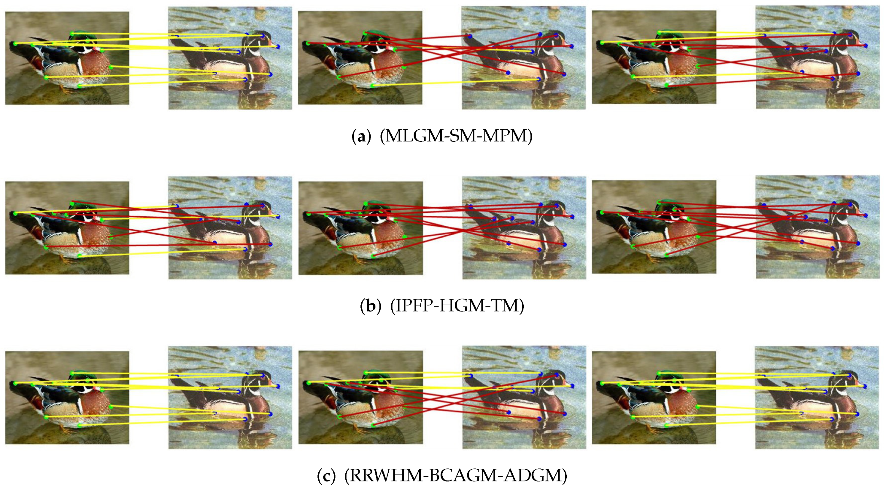
5.2. Face Dataset and Duck Dataset
In this section, we compare the performance of our method to other methods on the Face dataset and Duck dataset, which are the sub-datasets from Caltech-256 [
50]. These datasets contain images from specific classes: 109 face images, and 50 duck images. The ground truth is known for each graph pair. We chose 70 pairs of faces at random from the data set for testing, manually picked 10 feature points from each picture, and chose 20 photographs from each class at random as the training dataset for metric learning. The baseline was varied from 10 to 80 frames, and we tested all algorithms and obtained the average of the results. The accuracy and matching scores were obtained by averaging experiments of 10 frames to 80 frames. To make it more intuitive, we show several examples of matching results in
Figure 10 and
Figure 11. It can be seen that our algorithm performes better.
Figure 12 and
Figure 13 show that the MLGM method achieves the largest score value, and obtains more accurate matching results than other test methods. It also demonstrates that the compared approaches are easily affected by noise and distortion. The MLGM method can obtain a better matching result for the entire dataset.

