Abstract
In this work, we study the bifurcation and the numerical analysis of the nonlinear Benjamin-Bona-Mahony-KdV equation. According to the bifurcation theory of a dynamic system, the various kinds of traveling wave profiles are obtained including the behavior of solitary and periodic waves. Additionally, a two-level linear implicit finite difference algorithm is implemented for investigating the Benjamin-Bona-Mahony-KdV model. The application of a priori estimation for the approximate solution also provides the convergence and stability analysis. It was demonstrated that the current approach is singularly solvable and that both time and space convergence are of second-order precision. To confirm the computational effectiveness, two numerical simulations are prepared. The findings show that the current technique performs admirably in terms of delivering second-order accuracy in both time and space with the maximum norm while outperforming prior schemes.
Keywords:
BBM KdV equation; bifurcation theory; solitary wave; periodic wave; finite difference method MSC:
35Q51; 35C07; 65N06; 65N12
1. Introduction
Many real-world problems can be identified by various physical and mathematical models. It is found that numerous models are practically relevant to the nonlinear partial differential equations (NPDEs) and can be used to describe several realistic natural phenomena. There are several important mathematical models that can be implemented to the physical process in the scientific research area, and these gave rise to the appeal of the comprehensive study of nonlinear wave behaviors. The class of shallow water equations is one of the most crucial tools for modeling wave behaviors, which has been significantly applied to and integrated with the mathematical process for studying both atmospheric and oceanic models. Various phenomena of shallow water waves can be derived from NPDEs such as the Korteweg–De Vries (KdV) equation, the Benjamin-Bona-Mahony (BBM) or regularized long wave (RLW) equation and so forth [1,2,3,4]. The KdV Equation [1,2] was initially derived to investigate the dynamics of surface water waves in a channel. Later, the KdV equation was used in a variety of natural phenomena, such as longitudinal astigmatic waves, ion sound waves, and magnetic fluid waves. To explore small-amplitude long waves on the water surface and analyze nonlinear dispersion, Peregrine developed the BBM equation as an alternate model to the KdV Equation [3,4]. Furthermore, the BBM equation has been widely applied to many areas of the mechanism of physics phenomena. Here, we provide some scientific publications related to the KdV and RLW equations, which are relevant to the developing topics in [5,6,7,8,9].
The so-called Benjamin-Bona-Mahony-KdV (BBM-KdV) equation which has the model both BBM’s and KdV’s dispersive terms can be written as
where is a positive constant, and are real numbers; it is proposed by Bona and Smith [10]. In the case of , Equation (1) becomes to the BBM equation, while the KdV equation is formulated under the definition and . The BBM-KdV equation is one of the main topics to be studied in order to better understand the characteristic of wave motion. In [11], Lannes adapted the Dirichlet–Neumann operator to acquire the BBM-KdV-related model. Later, Mancas and Adams [12] obtained the local and the global well-posedness of the BBM-KdV equation. In addition to the theoretical studies, related researches on this equation are referred to in [13,14,15,16,17].
To understand the solution behaviors, finding the exact solutions is one of the main contributions to mathematical physics. In [18], Asokan and Vinodh obtained the soliton, kink, periodic, rational and traveling wave profiles for the BBM-KdV and related problems by applying the tanh–coth and transformed rational function procedures. Furthermore, Simbanefayi and Khalique [19] constructed the traveling wave solutions for the BBM-KdV equation based on the Lie symmetry method together with Jacobi elliptic function expansion. In fact, by using bifurcation theory from dynamical systems, all bifurcations and phase portraits of such traveling wave systems can be obtained in the parametric space. In [20], Z. Liu and C. Yang achieved the bifurcation of solitary waves of the KdV equation with the application of the bifurcation method of dynamical systems, while the explicit solitary wave solutions were also obtained under some parameter conditions. By applying the bifurcation method of dynamical systems, Chen and Li [21] studied the behavior of nonlinear waves through the generalized KdV-mKdV-like problem. Regarding the RLW equation, Lou [22] adopted the method of planar dynamical systems to furnish the smooth and non-smooth solutions of solitary and infinite periodic waves under different areas of parametric terms. Recently, the bifurcation and exact traveling wave solutions of the general RLW equation were successfully studied by Zheng et al. [23]. To our knowledge, traveling wave profiles caught by the BBM-KdV model have not been sufficiently studied before. As a consequence, the first objective in this paper is to analyze the bifurcation of all traveling wave solutions of the BBM-KdV equation by using methods from dynamical system theory. Various techniques can yield analytical answers, but because of their reliance on initial or boundary conditions, they are generally unusable. As a result, this signifies the necessity of the development in numerical techniques for solving the problems to understand the nature of solution behaviors.
Dutykh et al. solved the BBM-KdV equation using the traditional finite volume approach as well as explicit and implicit-explicit Runge–Kutta-type methods in [24]. For solving the BBM-Burgers equation with a high-order dissipative component, Lu et al. [25] proposed a finite element approach using adaptive moving meshes. The model can be used to solve equations containing spatial-time mixed derivatives and high-order derivative terms. Recently, the style of the numerical model for the BBM-KdV Equation [26] was investigated using a Fourier-spectral technique. In 2022, a technique based on conserved quantities was created to approximate and study the form, structure, and interaction characteristics of solitary waves represented by the BBM Equation [27]. Because the conserved parameters are invariant, there is no need to solve the corresponding complex nonlinear partial differential BBM equation to simulate the interactions of the solitary waves at the most merging occurrence. To identify the finite difference method, Rouatbi and Omrani [28] obtained two conservative difference schemes for solving the BBM-KdV equation; there are two-level nonlinear-implicit and three-level linear-implicit schemes. From the literature, most finite difference schemes (FDS) typically use the discretization for nonlinear terms as in Equation (1) at point in relation to the reformulation to gain analytical advantage, such as energy-preserving property, boundedness, convergence, and stability. Using the formulation with the Crank-Nicolson/Adams-Bashforth technique, many three-level FDS can develop and apply not only to the BBM-KdV equation, but also to the family of shallow water models [29,30,31,32,33,34,35,36,37]. This technique requires solving the initial numerical solution; that is, the Crank-Nicolson technique usually adopts two-level FDS. However, most of the two-level FDS are usually opted for solving nonlinear systems, which require high computation techniques. For example, Berardi and Difonzo [38] provided a novel numerical approach for solving the Richards’ equation inside the Gardner’s framework while maintaining second order in both space and time. They subsequently demonstrated that such a scheme converges to the precise solution, with the order of convergence preserved from the underlying quadrature formula. Therefore, the research study also aims to obtain a novel two-level FDS for the traveling wave solution of the BBM-KdV equation.
The remainder of the article is structured as follows. The wave transformation is introduced in Section 2 and is formulated with a planar dynamical system with the first integral. This will allow the BBM-KdV equation to be reduced to an ordinary differential equation. To approach traveling wave solutions, bifurcations and phase diagrams of the aforementioned planar dynamical system are also provided. The numerical simulation of the initial-boundary value problem for the BBM-KdV equation is covered in Section 3 of this article. To set up the problem, we make the following asymptotic assumptions on the solitary solution and its derivatives: and , as , for . A few numerical findings are presented in Section 4 to demonstrate the effectiveness of the suggested system while supporting and validating the theoretical analysis. Near the end of the article, a brief discussion of our research is presented.
2. Bifurcation and Phase Portraits
To understand the remodeling for the BBM-KdV problem, we investigate profiles of traveling wave solutions to the bifurcation formulated with the two-dimensional dynamic system. The ordinary differential equation
is first obtained by replacing the change , where , with the wave speed v. When integrating the equation with and neglecting integral constant, we have
We let , Equation (3) is equivalent to the following two-dimensional dynamic system
with the Hamiltonian function
where h is a constant.
Equation (5) imposes a phase portrait of the system (4) on the value of h. When h is varied, various families of orbits of the system (4) that have different dynamical behaviors can be obtained with regard to Equation (5). To determine the type of traveling wave solutions to Equation (1), we will evaluate the system’s bifurcations and phase diagram (4). From the theory of dynamical systems [39,40], a periodic orbit, a homoclinic orbit, and a heteroclinic orbit are found to correspond to the periodic wave solution, the solitary wave solution, and the kink or anti-kink wave solution, respectively. The equilibrium points of the system (4) can be found by equating the derivatives on the left-hand side to zero when the constant h is used as the bifurcation parameter. The system’s solutions
are found at the equilibrium locations. This gives two equilibrium points which are and . We now analyze the stability of each equilibrium point. At each given equilibrium point , the Jacobian matrix of the linearized system (4) is given by
and we have
By the theory of planar dynamical systems, we have the following qualitative analysis
- (i)
- A saddle point serves as the equilibrium point if .
- (ii)
- It serves as a center if and .
- (iii)
- It is a cusp point if and the Poincaŕe index, also known as the equilibrium point, is 0.
Consequently, we have
- (i)
- When . We see that and , thus the equilibrium point is a saddle point and is a center point.
- (ii)
- When . We have and , thus the equilibrium point is a center point and is a saddle point.
As a result, the bifurcation phase portraits of the system (4) shown in Figure 1 and Figure 2 are obtained. The system (4) has one equilibrium point for the case , and it is a cusp point (see Figure 3).
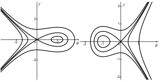
Figure 1.
The phase portraits of the system (4) when .
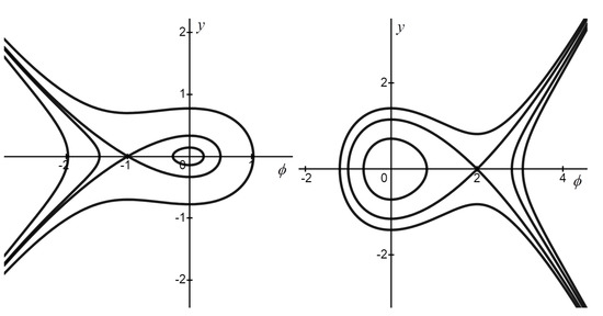
Figure 2.
The phase portraits of the system (4) when .
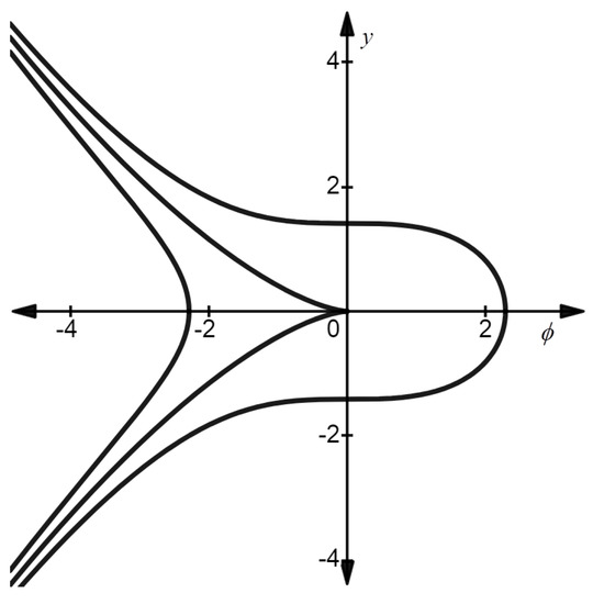
Figure 3.
The phase portrait of the system (4) when , and .
When , we obtain
- (i)
- (ii)
When , we obtain
- (i)
- (ii)
Here, some explicit expressions of traveling wave solutions of Equation (1) are given by letting the Hamiltonian constant . Clearly, Equation (5) can be written as
- (i)
- When , the system (4) has a homoclinic orbit in -plane. We obtain the smooth solitary wave solutionby substituting Equation (7) into and integrating them along the homoclinic orbit. This formulated solitary wave solution is shown in Figure 4 when and .
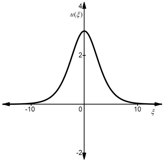 Figure 4. The solitary wave solution when , and .
 - (ii)
- When , the system (4) has a periodic orbit in -plane. Substituting Equation (7) into and integrating them along the periodic orbit, we have the periodic wave solutionThe periodic wave solution is shown in Figure 5 when , and .
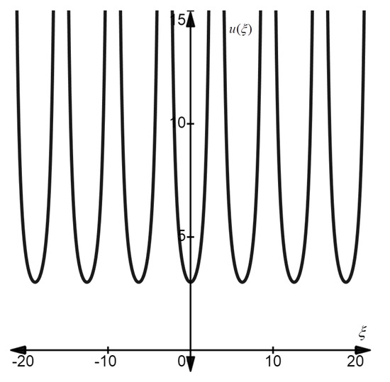 Figure 5. The periodic wave solution when , and .
Finite difference scheme
Through some special phase orbits, the analytic expression of the traveling wave solution of the BBM-KdV Equation (1) can be achieved. In this section, we contribute to the implementation of a numerical study of the BBM-KdV equation under solitary wave assumptions. Consider the initial-boundary value problem of the BBM-Burgers Equation (1) below with the starting constraint
that is a known smooth function and physical boundary conditions are
We first allow the solution domain to be covered by a uniform grid
before building the finite difference method for Equation (1) using Equations (8) and (9). Assuming is the discrete solution space, is the region inside that corresponds to the solitary wave circumstances as specified by
when and are true. For the numerical solution of a function u at the grid point , we indicate the notation . For simplicity, we use the following notations
For functions ,
may define the discrete inner product and the accompanying discrete -norm, whereas can establish the -norm.
To implement the acquired scheme, we regularly use the second-order accurate central difference approximations for linear operators in Equation (1). The second-order accurate Crank-Nicolson approximation in time derivative is applied to the entire scheme for the implementation process. To approximate the nonlinear term at the point by the Rubin and Graves linearization [41], we use the formula
Subsequently, we introduce the following linear implicit finite difference scheme for solving the BBM-KdV Equation (1) with Equations (8) and (9):
with an initial condition
and boundary conditions
The following energy-conserving characteristic is satisfied by the initial-boundary value problem (1) with Equations (8) and (9).
Theorem 1.
Proof.
So, is a constant function, that is
for all , as desired. □
Lemma 1.
For any two mesh functions , we have
Lemma 2.
Let . If there exists a positive constant C such that , then
Proof.
The proof is directly obtained by the Cauchy-Schwarz inequality and the assumption . □
Lemma 3.
Let . Then, we have
Proof.
Let , we can achieve
This completes the proof. □
Lemma 4
(discrete Sobolev’s inequality [42]). There exist two constants and such that
The subsequent theorem demonstrates that mass conservation exists in the difference scheme (10)–(12).
Proof.
Therefore, Equation (15) can be described from
This completes the proof. □
Theorem 3
Proof.
We employ mathematical induction and make the assumptions
and
for to demonstrate the boundedness. Taking in Equation (10) the inner product with , we obtain
According to Lemma 1, we have
By using the assumption (18) and Lemma 2, we note that
On the other hand, we observe that
where the assumption (18), the Cauchy-Schwarz inequality, and Lemma 3 are used. By incorporating Equations (21) and (22), Equation (20) can be estimated as
Let
Then Equation (23) can be rewritten as
If is adequately small, fulfilling and , then
Hence
which proves the precision of Equation (18). We complete the proof by using Lemma 4 to obtain . □
2.1. Solvability
In this section, the existence and the uniqueness of the present scheme are provided, which proves that the scheme (10)–(12) is uniquely solvable.
Proof.
Using mathematical induction, we can uniquely identify by an initial condition. Now, suppose be solved uniquely. Assume that and are the solutions of Equation (10). Let . Observe that satisfies
By taking the inner product of (24) with , using Lemma 1, we obtain
Applying Lemma 2 and Theorem 3, we have
and
Then, by Lemma 3, it yields
Therefore, if is small enough, then Equation (24) has the trivial solution. That is, is uniquely solvable. □
2.2. Convergence and Stability
Theorem 3 is used in this part to assess the convergence and stability of the scheme (10)–(12) in question. First, we introduce , where and are the solutions of Equation (1) with Equations (8)–(12), respectively. The following error equations are then obtained:
where denotes the truncation error. We note that holds as . Before conducting the convergence and the stability analysis, the following lemma is needed.
Lemma 5
(discrete Gronwall’s inequality [42]). Suppose that and are nonnegative functions and is nondecreasing. If and
then
The following theorem ensures that the current scheme will converge to the solution at the rate of .
Theorem 5.
Proof.
We obtain
by taking the inner product of Equation (26) and and using Lemma 1. Applying Theorem 3, Cauchy-Schwarz inequality, and the boundary conditions, we have
Similarly, we can acquire
Note that
Let
If is sufficiently small, which satisfies , then
By applying Lemma 5, we obtain
that is
Finally, by applying Lemma 4, we obtain
This completes the proof. □
Remark 1.
It is worth noting that our analysis still holds for the periodic boundary conditions. For more details, we refer the reader to [28].
3. Numerical Experiment
In this part, we will perform numerous numerical experiments to test the efficacy and validity of our earlier theoretical analyses. The parameters are configured to occur in unity, i.e., . To demonstrate the correctness of the proposed scheme, we will compare the error of the finite difference schemes established in [28], which are a second-order nonlinear scheme and a linear three-level scheme.
Scheme I Two-level nonlinear scheme [28]
Scheme II Three-level linearized scheme [28]
respectively. All of the above schemes are composed with these initial conditions
and boundary conditions
It is worth noting that when the approximated function is sufficiently smooth, Schemes I and II have second-order precision in both space and time when applying the Taylor expansion.
The method’s correctness is also tested by comparing numerical results to precise solutions using the -norm , defined by
The - and - norms were used to illustrate the inaccuracy of the numerical solutions in the sense of and norms, respectively, to demonstrate the correctness of our approach. In addition, we determine the rate of convergence using two grids and the formula
Our numerical simulation research for the topic of BBM-KdV equation extension may be separated into two cases:
Example 1.
The nonhomogenous BBM-KdV Equation [28].
Consider the following BBM-KdV equation
in the first example. To check the order of correctness, we adjust the non-homogeneous function g to match the precise answer
For Equation (37), the initial condition leading to the precise solution is as follows:
as to the periodic boundary conditions .
The present scheme is tested numerically over the space interval and the time interval under the same setting as in [28]. The spatial and temporal step sizes are selected to be small enough that the dominant error is based on just one component. The comparison and spatial convergence orders in error norms of numerical solution are reported in Table 1 using small temporal step size and to . The present scheme is convergent in the sense of -norm with the second order in space as expected. According to our observation, the present scheme provides a more significantly accurate numerical resolution than that of the other schemes with at least improvement, as seen in Table 1. In addition, Table 2 lists the comparison of the error norms and the order of the temporal convergence by setting and to . The findings indicate that these behavioral tendencies are comparable to those shown in Table 1; further, we can observe that the accuracy can be improved up to and as in Scheme I and Scheme II, respectively, when and are used. Furthermore, Table 1 and Table 2 clearly illustrate that the rate of convergence of our method is virtually second order in time and space, which is consistent with the reasoning given in Theorem 5. Moreover, it is clearly reported in Table 1 and Table 2 that the rate of convergence of our scheme shows almost second-order in time and space, which is in good agreement with the argument discussed in Theorem 5.

Table 1.
Error comparison and spatial convergence orders in -norm using and .
Table 2.
Error comparison and temporal convergence orders in -norm using and .
Additionally, Figure 6 displays the numerical solutions and the absolute distribution from to the extended final time , when and are used. It can be observed that the present scheme provides the efficient resolution of analytical solution which is aligned with the analytical solution (38).
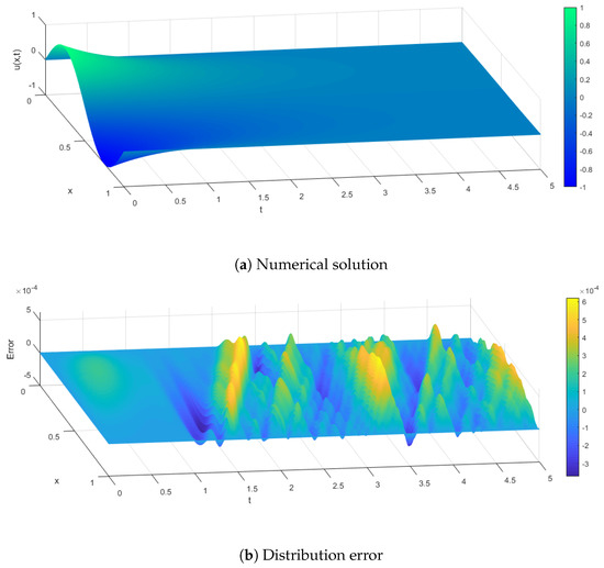
Figure 6.
Numerical solution and distribution error with and and to 5.
Example 2.
The single solitary wave: the BBM-KdV equation.
In this example, we will look at the BBM-KdV equation
The analytical solution to the BBM-KdV equation is as follows:
which stands for a single solitary wave having amplitude centered at with velocity and . As a result, the initial condition corresponding to the precise solution is provided for Equation (37) as follows:
and the boundary conditions (12).
The current approach is quantitatively tested in the simulation for the case of with over the space interval and the time interval . The average and maximum errors under different step sizes and at the final time are reported in Table 3. It is observable that the accuracy of the proposed scheme is compatible with the two-level nonlinear Scheme I, and is considerably better than the linear Scheme II with at least improvement. However, according to the data shown in the table, the second-order rate of convergence is confirmed, which is in significant relation to the theoretical expectation for each scheme. In Figure 7, we simulate the numerical solutions and their distribution errors when are used, as produced by the present scheme, Schemes I and II, respectively. According to the results, each scheme may perfectly mimic the exact solution, with the largest inaccuracy occurring around the maximum displacement of the wave amplitude.
Table 3.
Error comparison and temporal convergence orders in -norm using at .
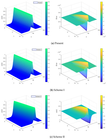
Figure 7.
Numerical solutions and distribution errors with and to 10 (a) Present (b) Scheme I (c) Scheme II.
The existing finite difference formulation for the BBM-KdV equation will now be demonstrated to control the shape of a single soliton over time. The suggested technique is devoted to a numerical model by monitoring wave motion simulations up to . Figure 8 shows the approximate solution configuration; the wave characteristic is plainly visible at this stage. Because of the reduced left-tail oscillation, the current approach produces a more stable outcome. An intriguing aspect of these results is that an error value is minimized and an oscillation is significantly reduced.
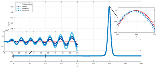
Figure 8.
Numerical solutions with and to 200.
Finally, each scheme is applied to the studied method to verify to the mathematical process to verify the conservation of the numerical model. We monitor the numerical simulations under the same setting over the computational region and the time interval to support the mass-preserving property as derived in Theorem 15.
The findings demonstrate that the mobility constant deviates significantly from the precise value stated in Table 4. However, the mass quantity is more precisely preserved in time at least six digits when the present scheme and Scheme I are applied, while Scheme II can preserve the mass quality only five digits.
Table 4.
The quantities of and its errors using at various time.
4. Conclusions
In conclusion, we effectively obtained a bifurcation analysis and a numerical strategy for finding accurate and numerical solutions to the BBM-KdV problem. We obtained a class of exact solutions comprising solitary wave and periodic wave solutions via the bifurcation theory dynamical system by applying the approach of planar dynamical systems. Furthermore, we used a two-level linear implicit finite difference approach to solve the BBM-KdV problem numerically. The stability and convergence analyses were carried out in the analytical report. Furthermore, the accuracy and stability of the numerical approach for the solution to the BBM-KdV equation may be checked by using the exact solution; the prior benchmark solutions are the nonhomogeneous BBM-KdV equation with periodic boundary conditions and the single solitary wave solution. The numerical trials indicate that the current approach is accurate and efficient for delivering adequate resolution, and that it is much superior to previously known methods. The numerical experiments reveal that our suggested approach may be used to analyze and verify the convergence rate as well as the mass-preserving quality.
Author Contributions
Conceptualization, T.S., K.P. and B.W.; Investigation, T.S., K.P. and B.W.; Methodology, T.S., K.P. and B.W.; Project administration, T.S.; Resources, B.W.; Software, T.S. and B.W.; Validation, T.S. and K.P.; Visualization, K.P. and B.W.; Writing—original draft, T.S. and B.W.; Writing—review & editing, T.S. and B.W. All authors have read and agreed to the published version of the manuscript.
Funding
This research was supported by the Centre of Excellence in Mathematics, Ministry of Higher Education, Science, Research and Innovation, the National Research Council of Thailand (NRCT) under Grant No. N42A650208 and Chiang Mai University, Thailand.
Data Availability Statement
The data that support the findings of this study are available within the article.
Conflicts of Interest
The authors declare no conflict of interest.
References
- Benjamin, T.B.; Bona, J.L.; Mahony, J.J. Model equations for long waves in nonlinear dispersive systems. Trans. Roy. Soc. (Lond.) Ser. A 1992, 272, 47–78. [Google Scholar]
- Korteweg, D.J.; de Vries, G. On the change of form of long waves advancing in a rectangular canal, and on a new type of long stationary waves. Philos. Mag. 1895, 39, 422–443. [Google Scholar] [CrossRef]
- Peregrine, D.H. Calculations of the development of an undular bore. J. Fluid Mech. 1966, 25, 321–330. [Google Scholar] [CrossRef]
- Peregrine, D.H. Long waves on a beach. J. Fluid Mech. 1967, 27, 815–827. [Google Scholar] [CrossRef]
- Musette, M.; Lambert, F.; Decuyper, J. Soliton and antisoliton resonant interactions. J. Phys. A Math. Gen. 1987, 20, 6223–6235. [Google Scholar] [CrossRef]
- Easwaran, C.; Majumbar, S. The evolution of perturbations of the renormalized long wave equation. J. Math. Phys. 1988, 29, 390–392. [Google Scholar] [CrossRef]
- Camassa, R.; Holm, D. An integrable shallow water wave equation with peaked solitons. Phys. Rev. Lett. 1993, 71, 1661–1664. [Google Scholar] [CrossRef]
- Biswas, A. 1-Soliton solution of Benjamin-Bona-Mahoney equation with dual-power law nonlinearity. Commun. Nonlinear Sci. Numer. Simul. 2010, 15, 2744–2746. [Google Scholar] [CrossRef]
- Biswas, A. 1-Soliton solution of the B(m,n) equation with generalized evolution. Commun. Nonlinear Sci. Numer. Simul. 2009, 14, 3226–3229. [Google Scholar] [CrossRef]
- Bona, J.L.; Smith, R. The initial-value problem for the Korteweg-de Vries equation. Philos. Trans. R. Soc. Lond. A Math. Phys. Eng. Sci. 1975, 278, 555–601. [Google Scholar] [CrossRef]
- Lannes, D. The Water Waves Problem: Mathematical Analysis and Asymptotics; American Mathematical Society: Providence, RI, USA, 2013. [Google Scholar]
- Mancas, S.C.; Adams, R. Elliptic solutions and solitary waves of a higher order KdV–BBM long wave equation. J. Math. Anal. Appl. 2017, 452, 1168–1181. [Google Scholar] [CrossRef]
- Maxworthy, T. Experiments on collisions between solitary waves. J. Fluid Mech. 1976, 76, 177–185. [Google Scholar] [CrossRef]
- Francius, M.; Pelinovsky, E.N.; Slunyaev, A.V. Wave dynamics in nonlinear media with two dispersionless limits for long and short waves. Phys. Lett. A 2001, 280, 53–57. [Google Scholar] [CrossRef]
- Besse, C.; Noble, P.; Sanchez, D. Discrete transparent boundary conditions for the mixed KDV-BBM equation. J. Comput. Phys. 2017, 345, 484–509. [Google Scholar] [CrossRef]
- Bona, J.L.; Carvaxal, X.; Panthee, M.; Scialom, M. Higher-order Hamiltonian model for unidirectional water waves. J. Nonlinear Sci. 2018, 28, 543–577. [Google Scholar] [CrossRef]
- Dutykh, D.; Pelinovsky, E. Numerical simulation of a solitonic gas in KdV and KdV–BBM equations. Phys. Lett. A 2014, 378, 3102–3110. [Google Scholar] [CrossRef]
- Asokan, R.; Vinodh, D. Soliton and Exact Solutions for the KdV–BBM Type Equations by tanh–coth and Transformed Rational Function Methods. Int. J. Appl. Comput. Math. 2018, 4, 1–20. [Google Scholar] [CrossRef]
- Simbanefayi, I.; Khalique, C.M. Travelling wave solutions and conservation laws for the Korteweg–de Vries–Bejamin–Bona–Mahony equation. Results Phys. 2018, 8, 57–63. [Google Scholar] [CrossRef]
- Liu, Z.; Yang, C. The application of bifurcation method to a higher-order KdV equation. J. Math. Anal. Appl. 2002, 275, 1–12. [Google Scholar] [CrossRef]
- Chen, Y.; Li, S. New Traveling Wave Solutions and Interesting Bifurcation Phenomena of Generalized KdV-mKdV-Like Equation. Adv. Math. Phys. 2021, 2021, 4213939. [Google Scholar] [CrossRef]
- Lou, Y. Bifurcation of travelling wave solutions in a nonlinear variant of the RLW equation. Commun. Nonlinear Sci. Numer. Simul. 2007, 12, 1488–1503. [Google Scholar] [CrossRef]
- Zheng, H.; Xia, Y.; Bai, Y.; Wu, L. Travelling wave solutions of the general regularized long wave equation. Qual. Theory Dyn. Syst. 2021, 20, 1–21. [Google Scholar] [CrossRef]
- Dutykh, D.; Katsaounis, T.; Mitsotakis, D. Finite volume methods for unidirectional dispersive wave models. Int. J. Numer. Methods Fluids 2013, 71, 717–736. [Google Scholar] [CrossRef]
- Lu, C.; Gao, Q.; Fu, C.; Yang, H. Finite element method of BBM-Burgers equation with dissipative term based on adaptive moving mesh. Discret. Dyn. Nat. Soc. 2017, 2017, 3427376. [Google Scholar] [CrossRef]
- Bona, J.L.; Chen, H.; Hong, Y.; Karakashian, O. Numerical Study of the Second–Order Correct Hamiltonian Model for Unidirectional Water Waves. Water Waves 2019, 1, 3–40. [Google Scholar] [CrossRef]
- You, X.; Xu, H.; Sun, Q. Analysis of BBM solitary wave interactions using the conserved quantities. Chaos Solitons Fractals 2022, 155, 111725. [Google Scholar] [CrossRef]
- Rouatbi, A.; Omrani, K. Two conservative difference schemes for a model of nonlinear dispersive equations. Chaos Solitons Fractals 2017, 104, 516–530. [Google Scholar] [CrossRef]
- Omrani, K.; Ayadi, M. Finite difference discretization of the Benjamin-Bona-Mahony-Burgers’ equation. Numer. Methods Partial. Differ. Equ. 2008, 24, 239–248. [Google Scholar] [CrossRef]
- Janwised, J.; Wongsaijai, B.; Mouktonglang, T.; Poochinapan, K. A modified three-level average linear-implicit finite difference method for the Rosenau-Burgurs equation. Adv. Math. Phys. 2014, 2014, 734067. [Google Scholar] [CrossRef]
- Wongsaijai, B.; Poochinapan, K. A three-level average implicit finite difference scheme to solve equation obtained by coupling the Rosenau-KdV equation and the Rosenau-RLW equation. Appl. Math. Comput. 2014, 245, 289–304. [Google Scholar] [CrossRef]
- Poochinapan, K.; Wongsaijai, B.; Disyadej, T. Efficiency of high-order accurate difference schemes for the Korteweg-de Vries equation. Math. Probl. Eng. 2014, 2014, 862403. [Google Scholar] [CrossRef]
- He, D.; Pan, K. A linearly implicit conservative difference scheme for the generalized Rosenau–Kawahara-RLW equation. Appl. Math. Comput. 2015, 271, 323–336. [Google Scholar] [CrossRef]
- He, D. New solitary solutions and a conservative numerical method for the Rosenau–Kawahara equation with power law nonlinearity. Nonlinear Dyn. 2015, 82, 1177–1190. [Google Scholar] [CrossRef]
- Wang, X.; Dai, W. A three-level linear implicit conservative scheme for the Rosenau-KdV-RLW equation. J. Comput. Appl. Math. 2018, 330, 295–306. [Google Scholar] [CrossRef]
- Nanta, S.; Yimnet, S.; Poochinapan, K.; Wongsaijai, B. On the identification of nonlinear terms in the generalized Camassa-Holm equation involving dual-power law nonlinearities. Appl. Numer. Math. 2021, 160, 386–421. [Google Scholar] [CrossRef]
- Chousurin, R.; Mouktonglang, T.; Wongsaijai, B. Performance of compact and non-compact structure preserving algorithms to traveling wave solutions modeled by the Kawahara equation. Numer. Algorithms 2020, 85, 523–541. [Google Scholar] [CrossRef]
- Berardi, M.; Difonzo, F.V. A quadrature-based scheme for numerical solutions to Kirchhoff transformed Richards’ equation. J. Comput. Dyn. 2022, 9, 69–84. [Google Scholar] [CrossRef]
- Chow, S.N.; Hale, J.K. Method of Bifurcation Theory; Springer: New York, NY, USA, 1981. [Google Scholar]
- Guckenheimer, J.; Holmes, P.J. Nonlinear Oscillations, Dynamical Systems and Bifurcations of Vector Fields; Springer: New York, NY, USA, 1983. [Google Scholar]
- Rubin, S.G.; Graves, R.A. Cubic Spline Approximation for Problems in Fluid Mechanics; NASA TR R-436; NASA: Washington, DC, USA, 1975.
- Zhou, Y. Application of Discrete Functional Analysis to the Finite Difference Method; International Academic Publishers: Beijing, China, 1990. [Google Scholar]


Publisher’s Note: MDPI stays neutral with regard to jurisdictional claims in published maps and institutional affiliations. |
© 2022 by the authors. Licensee MDPI, Basel, Switzerland. This article is an open access article distributed under the terms and conditions of the Creative Commons Attribution (CC BY) license (https://creativecommons.org/licenses/by/4.0/).