Investigation of Efficient Optimization Approach to the Modernization of Francis Turbine Draft Tube Geometry

Abstract

The installation of new and revitalization of existing hydropower requires the optimal design of hydraulic turbine parts, which were previously mostly based on simplified analytical methods and engineering practices. With the increase in computational power, optimization methods now present an effective approach to the improvement of the geometry of turbine parts, thus enabling fine geometry-tuning adjustments of site specifics. However, despite continually increasing computational power, such numerical optimizations still require substantial resources and time. Therefore, in the proposed paper, extensive analysis of different numerical simplifications was conducted to determine the best trade-off between accuracy and the required computational resources for draft tube optimization. Additionally, the influence of geometry parametrization in terms of greater geometry flexibility, different goal functions, and optimization parameters was investigated. Within the considered constraints, a novel draft tube geometry was obtained, with the elbow displacements toward the draft tube exit, a shape that could not be obtained with the usual draft tube parametrization. It was also observed that geometry improvements for a single operating point did not provide improvements for other operating points. The obtained findings regarding the numerical and optimization setup can be used as guidelines for future optimization research, where multiobjective optimization for multiple operating points should be further investigated.

1. Introduction

Hydropower is one of the oldest renewable resources and although the continuous development of new renewable energy sources might reduce its relative competitiveness, hydropower still has a promising future due to emerging sustainable energy policies [1]. In the domain of hydroelectric energy, new trends are aimed at the utilization of small and micro-hydroelectric power plants [2,3], with an increasing need for pumped storage solutions [4]. Therefore, considerable research and development are being conducted to enhance the design of existing and new hydroelectric power plants [5,6,7].

The efficiency of a hydraulic turbine can be increased with the installation of a draft tube, as it converts the remaining kinetic energy from the water leaving the runner into static pressure. Traditional draft tubes were constructed using simplified analytical methods, experimental prototypes, and the best engineering practices. However, as computational capabilities have improved, Computational Fluid Dynamics (CFD) can be used to investigate optimal designs, providing flexibility and enabling engineers to obtain improved designs that ultimately increase turbine efficiency and renewable energy exploitation [8]. These tools are increasingly being considered in the design processes of new and the modernization of existing hydroelectric power plants. An overview of draft tube development was given by Abbas and Kumar [9].

A numerical analysis of 256 different Francis turbine draft tube designs was conducted by Sosa et al. [10] to obtain an improved design. The influence of the intake and draft tube geometry parameters of Kaplan micro turbines on turbine efficiency was evaluated using LES simulations in Amano and Abbas [11]. In Schiffer et al. [12], an evaluation of different draft tube designs for Kaplan turbines was conducted to achieve a balance between construction costs and turbine efficiency. Arispe et al. [13] conducted CFD analyses for four different parametrization approaches to a Francis turbine draft tube elbow. Since CFD simulations are expensive, design improvements are frequently carried out using the Design of Experiment (DoE) approach, which simplifies the considered problem by providing a limited number of significant combinations of design parameters from which the meaningful behavior of the investigated design problem can be extracted. The DoE approach and response surface method were used by chol Nam et al. [14] to obtain an improved draft tube design with an increased pressure recovery factor. In Favrel et al. [15], the DoE and analysis of means (ANOM) approaches were used to obtain the optimal design that can reduce flow instabilities and pressure fluctuations.

Optimization methods offer an intriguing solution to the design improvement problem, with the optimization algorithm selecting the design parameters for subsequent CFD evaluations to obtain the optimal solution. Local optimization methods are used to reduce the number of costly goal function evaluations and although local methods have faster convergence, they can obtain only local optima if the search is not conducted in the vicinity of global optima. As a result, global optimization methods are increasingly being used to optimize hydraulic parts [16,17]. In a paper by Eisinger and Ruprecht [18], the SIMPLEX method and a genetic algorithm (GA) were used for draft tube optimization, whereas in Fleischli et al. [19], an evolutionary algorithm (EA) and adjoint method were used. The metamodel-assisted evolutionary algorithm (MAEA) was used in a study by McNabb et al. [17], where after enough individuals were evaluated, the metamodel was used for the pre-evaluation of further offspring to reduce computational time. Particle swarm optimization (PSO) was used in a study by Moravec and Rudolf [20] to optimize a hydraulic diffuser. In a paper by Lyutov et al. [21], the coupled multiobjective optimization of the runner and draft tube geometry was conducted for geometry scaled down to a 1 m unit diameter. A multiobjective genetic algorithm (MOGA) was used to increase efficiency for multiple operating points.

It is evident that due to the improved computational capabilities, stochastic optimization methods are becoming more popular; however, to the best of the authors’ knowledge, no general agreement on numerical setup and optimization parameters has previously been reached. When choosing numerical and optimization parameters for the optimization procedure, a trade-off must be made between accuracy and robustness. Since higher-order numerical models require high-quality numerical grids to satisfy convergence criteria, striving for excellent accuracy implies increased computational demands. This can be met if the user is able to improve the mesh after obtaining the preliminary simulation results. However, because specific adjustments cannot be made during the optimization procedure, robust numerical parameters are required to satisfy the convergence criteria for a wide range of simulations. The evaluation of all designs, rather than rejecting them due to a convergence penalty, is valuable information for the optimization method since it provides information regarding the direction of further searches. Furthermore, by following an optimization procedure, several of the best solutions can be further evaluated with higher accuracy simulations to validate the obtained designs. Therefore, this study investigates various numerical and optimization approaches in order to provide an optimization framework with the best trade-off between simulation accuracy, robustness, and computational demands. This paper is organized as follows. In the second section, a methodology overview is given. The geometrical and performance characteristics of the considered turbine and draft tube are given. Additionally, an overview of the investigated numerical parameters considered for obtaining robust simulations for the optimization procedure is presented. An overview of the used optimization method is given, with a description of the investigated optimization parameters. The results of the conducted investigations are presented in the third section, followed by a brief discussion and conclusion.

2. Methodology

2.1. Turbine Operational and Geometrical Characteristics

The hydropower plant considered in this work is HPP Rijeka, with an installed capacity of 36.8 MW. It is located on the Rječina River, Rijeka, Croatia, and has an artificially built Valići reservoir V = 6 × 10${}^5$ m${}^3$. The Rječina River has torrential behavior, where the average annual flow is 7.48 m${}^3$/s [22]. Two Francis turbines are located in the underground engine room at a height of 1.6 m above sea level with an installed flow of 2 × 10.5 m${}^3$/s. The considered turbine has an elbow-type draft tube defined by 16 reference sections. The first three cross-sections have a circular shape that transitions into rounded rectangles (Figure 1). The considered sections are oriented along the curved centerline.

In general, the revitalization of the existing draft tube was conducted with minimal alterations to the original design in terms of vertical expansion or extension since the requirements for additional operations such as excavation would increase the expenses. In the works by Skotak et al. [23] and Fleischli et al. [19], a new draft tube design was kept within the dimensions of the original draft tube. In this paper, two different approaches were considered regarding the geometry constraints. In the first case, it was mandated that the optimized design was kept within the original draft tube limits, and in the second case, additional excavation was allowed; dimensional changes (i.e., increases) to the geometry were allowed within a specified relative percentage range compared to the initial design. The second case was considered as it can be argued that the additional expenses required for the excavation during the modernization procedure could be beneficial in the long term, considering the improvements to the geometry.

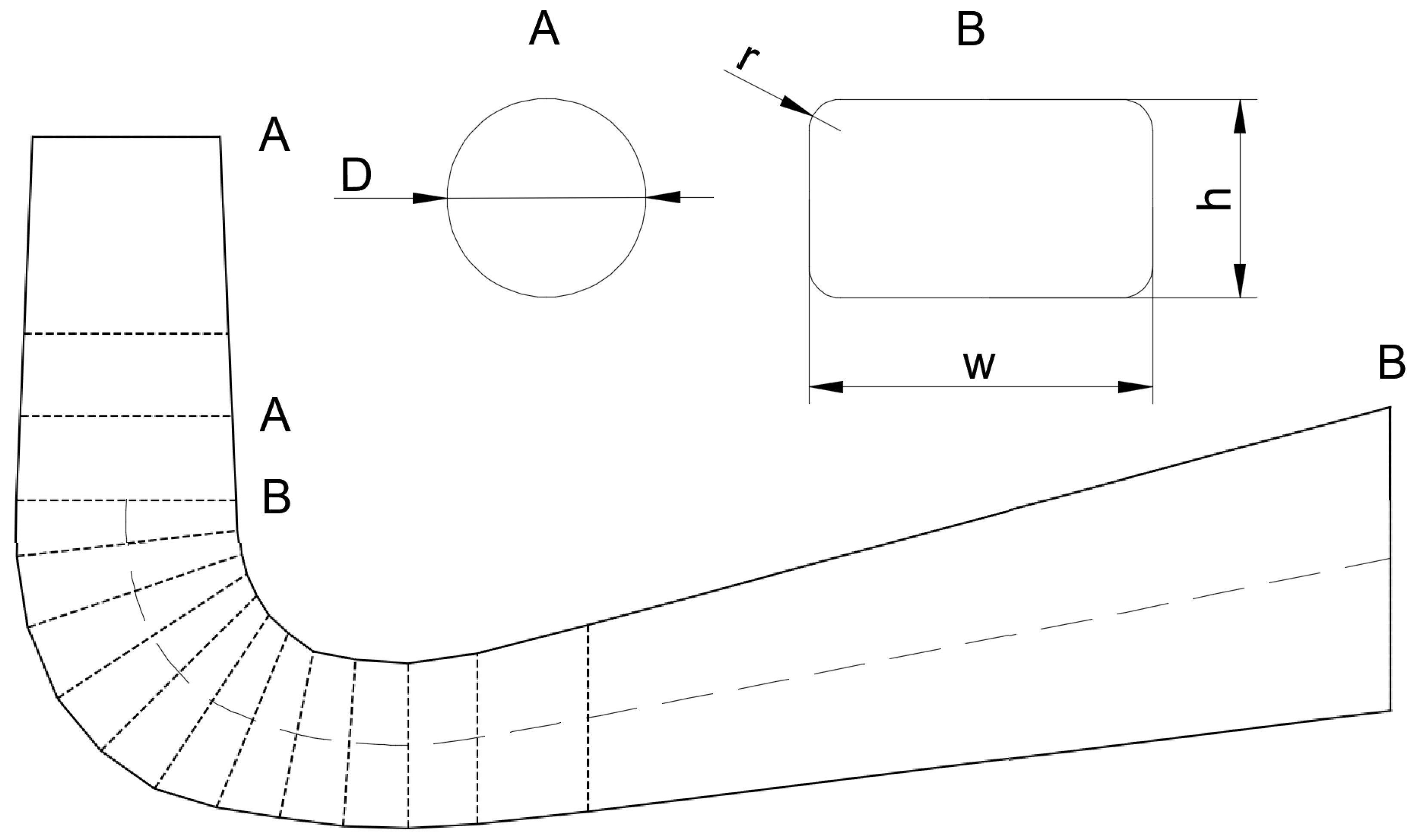
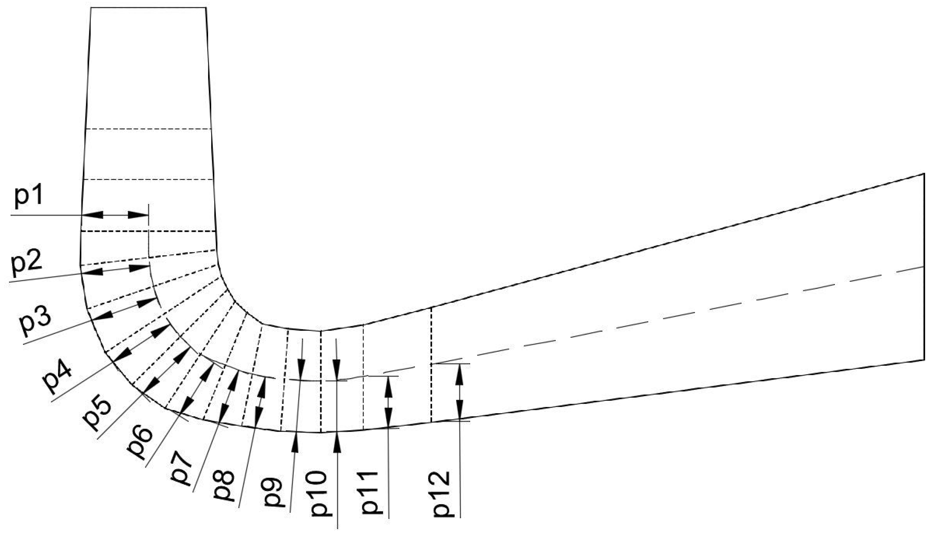
2.2. Geometry Parametrization

To reduce the complexity of the optimization problem and, additionally, the scope of the changes to the original design, it was decided to change only the height of the lower section of the draft tube. Additionally, only the rounded rectangle cross-sections, i.e., sections 4–15, were chosen for the modification. The last profile was also fixed since its alteration would require additional changes to the infrastructure at the draft tube exit. The parameter defining the geometry was the distance of the lower profile from the centerline at each section, which thus resulted in 12 unique parameters chosen as the optimization variables (Figure 2). The geometry for the proposed workflow was created with Python using the FreeCAD Conda package version 0.20.1.

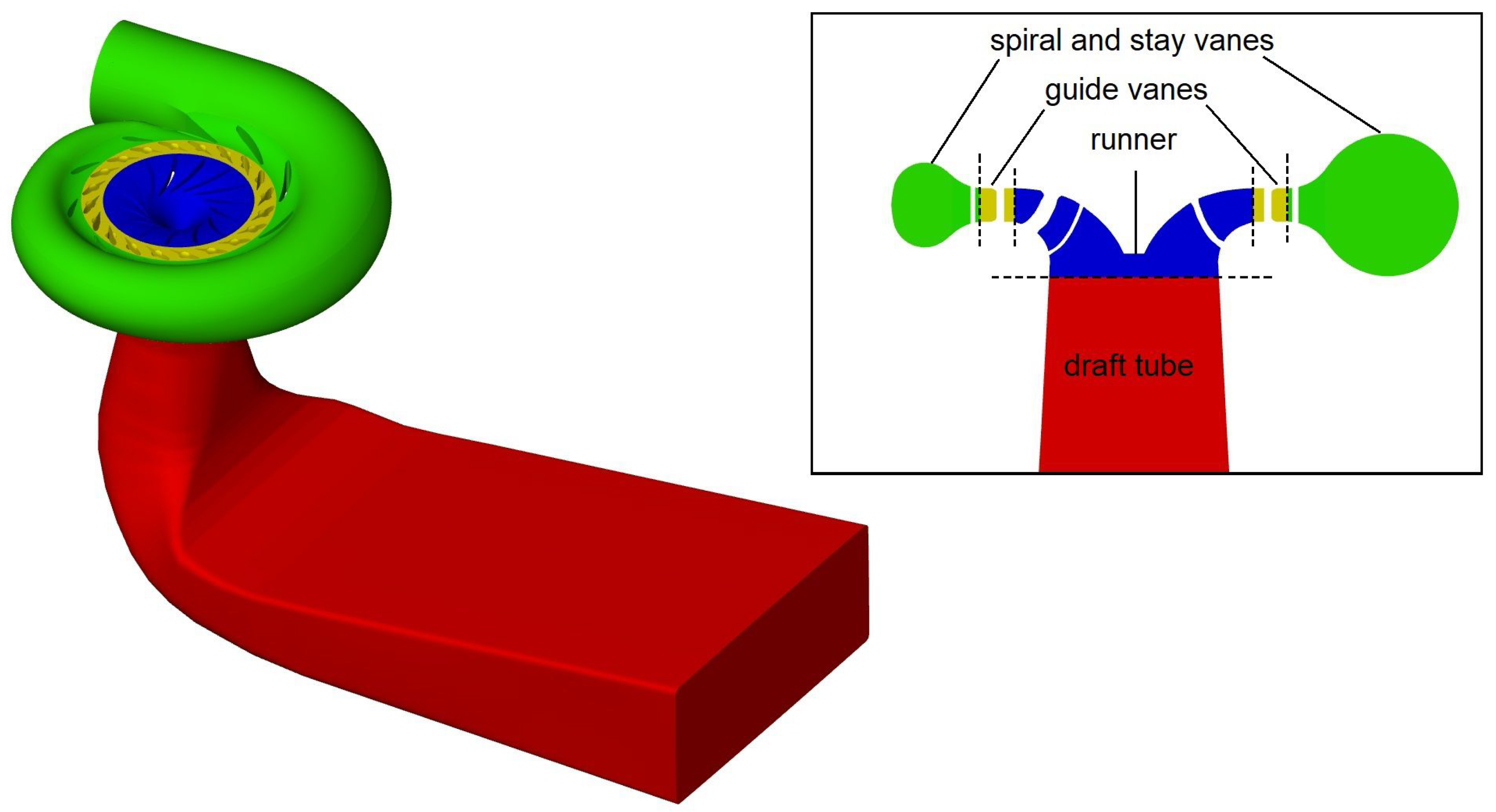
2.3. Computational Domain and Grid

Due to the potential significant variability of the geometry during the optimization approach’s geometry generation procedure, an unstructured mesh was chosen to provide the robustness required to properly describe the different designs that may be encountered. Polyhedral, hybrid polyhedral-hexahedral, hexahedral, and tetrahedral grids were all investigated. Ansys Fluent meshing 21.1 software was used for the model meshing. To achieve the required robustness for the optimization procedure, the minimum and maximum element sizes were set as the only mesh-generation governing parameters. Additional domain refinements were not employed. The coarse mesh had a minimum allowed element size of 0.1 mm and a maximum allowed element size of 100 mm. The first layer’s thickness was set to 1 mm with three boundary layers in total so as to achieve an average $y^{+}\approx 100$. A preliminary assessment of the considered mesh types revealed that the hybrid polyhedral-hexahedral mesh had the fewest elements (

Table 1. Number of elements for different mesh types.

Mesh Type	No. Elements
hexahedral	646029
polyhedral-hexahedral	242106
polyhedral	288872
tetrahedral	1052053

) with the shortest computational time; hence, it was adopted for this study.

Subsequently, a mesh sensitivity study was conducted. Three grids, namely coarse, medium, and fine, were considered. The grids were generated by employing a global refinement ratio of 1.5. The relevant parameters and GCI results for each of the considered grids are shown in

Table 2. Mesh details and GCI results for the $C_p$ and $C_d$ coefficients.

Mesh	Min Size	Max Size	No.	${\mathit{C}}_{\mathit{p}}$		${\mathit{C}}_{\mathit{d}}$
	[mm]	[mm]	Elements	e [%]	GCI [%]	e [%]	GCI [%]
Coarse	0.1	100	242106	-	-	-	-
Medium	0.066	66.6	428295	6.465	1.421	4.289	8.140
Fine	0.044	44.4	967650	0.976	0.172	2.521	4.784

. Two variables were assessed: the pressure recovery coefficient, $C_p$, and the loss coefficient, $C_d$. The pressure recovery coefficient describes how much kinetic energy is successfully converted to static pressure and is defined as

$$C_p=\frac{p_{2stat}-p_{1stat}}{\frac{1}{2}\rho v^2}$$

(1)

The drag coefficient is defined as

$$C_d=\frac{p_{1tot}-p_{2tot}}{\frac{1}{2}\rho v^2}$$

(2)

where $p_{stat}$ is the static pressure and $p_{tot}$ is the total pressure; subscripts 1 and 2 indicate the inlet and outlet, respectively; $\rho$ is the water density; and v is the absolute velocity. In both cases, the results were in the asymptotic range of convergence, i.e., $GC{I}_{m,f}/(r^p·GC{I}_{c,m})=0.99$ and $GC{I}_{m,f}/(r^p·GC{I}_{c,m})=1.026$ for $C_p$ and $C_d$, respectively. Considering this, and in order to reduce the computational time, the coarsest mesh was deemed adequate for future simulations.

2.4. Numerical Settings and Validation

Navier–Stokes equations are coupled partial differential equations consisting of continuity, momentum, and energy equations, which describe the incompressible fluid flow under the assumption of the fluid continuum. The Reynolds-averaged Navier–Stokes models use the Reynolds averaging method in which the flow variables are the result of time averaging. In Cartesian coordinates, the averaged isothermal momentum and continuity equations can be written as

$$\frac{\partial }{\partial x_i}\left(\rho {\overline{u}}_i\right)=0$$

(3)

$$\frac{\partial }{\partial t}\left(\rho {\overline{u}}_i\right)+\frac{\partial }{\partial x_j}\left(\rho {\overline{u}}_i{\overline{u}}_j\right)=-\frac{\partial }{\partial x_i}\overline{p}+\frac{\partial }{\partial x_j}\left[\mu \left(\frac{\partial {\overline{u}}_i}{\partial x_j}+\frac{\partial {\overline{u}}_j}{\partial x_i}-\frac{2}{3}{\delta }_{ij}\frac{\partial {\overline{u}}_l}{\partial x_l}\right)-\rho \overline{u_i^{{}^{\prime }}{u}_j^{{}^{\prime }}}\right]$$

(4)

where $\rho$ represents the density, t is the time, $x_i$ are the Cartesian coordinates, $u_i$ are components of the velocity, $\mu$ is the molecular viscosity, $\rho \overline{u_i^{{}^{\prime }}{u}_j^{{}^{\prime }}}$ represents the Reynolds stresses, and ${\delta }_{ij}$ is the Kronecker delta. Variables with overlines represent mean values.

Since computing the exact solutions to the Navier–Stokes equations is typically not feasible, different turbulent models have been developed to simplify the calculations. Each model introduces specific assumptions. The choice of turbulent model varies in the literature and is typically governed by the methodology employed to model the flow; the most common are the standard $k-ϵ$ [21,24,25], $k-\omega$ standard [10], and $k-\omega$ SST [12,13,14,15] models. Among them, however, the $k-\omega$ SST turbulence model is predominant because it accurately predicts flow with strong pressure gradients and separation and is applicable to a wide range of y+ values. The $k-\omega$ SST model is a two-equation turbulence model that uses two additional transport equations. In the near wall region, the SST model defaults to the $k-\omega$ implementation, whereas the $k-ϵ$ model is employed far from the wall. This hybrid approach offers flexibility for complex problems. Given the wide range of geometries that an optimization algorithm can generate, it would be difficult to ensure that all grids satisfy strict mesh conditions near the wall for the $k-ϵ$ and $k-\omega$ models. Meanwhile, when the y+ range is 1–100, the $k-\omega$ SST model produces acceptable results. Several preliminary simulations conducted in this study revealed no significant difference in computational time between the $k-ϵ$ standard and $k-\omega$ SST models; therefore, the $k-\omega$ SST model was chosen as the default turbulent model due to its robustness. More details regarding the $k-\omega$ SST model implementation can be found in the paper by Menter et al. [26].

Two approaches were considered to investigate the influence of boundary conditions. First, a uniform inflow velocity was prescribed through a mass flow inlet boundary condition. Due to the constant inflow value and symmetric draft tube design, simplification can be made by using only one-half of the computational domain and applying the symmetry condition, thus significantly reducing the computational time. The second approach used a characteristic velocity profile obtained at the runner outlet (draft tube inlet) of the original turbine model, which had a constant value of 10 m${}^3$/s at the inlet. The considered velocity profile was obtained from the study in [27], where fluid flow analysis through the entire turbine was performed and validated with in situ measurements. For this case, the whole draft tube geometry was used since the obtained velocity profile was not symmetrical.

Table 3. Boundary conditions for the two considered cases.

	Case 1	Case 2
Inlet	mass-flow inlet	velocity profile
Outlet	pressure outlet	pressure outlet
Wall	no-slip	no-slip
Symmetry	yes	-

provides an overview of the boundary conditions that were used. Although the uniform inlet velocity is not a realistic representation of the fluid flow in a draft tube, it enables quick investigations of the numerical settings and optimal optimization parameters. The velocity profile was used for the final geometry optimization.

An assessment of the numerical setup was conducted for different pressure-velocity couplings, numerical schemes, and residuals. In order to determine the importance of the residuals, simulations were first conducted with the convergence criteria set for all residuals to 10${}^{-5}$. In the second case, the continuity residual was lowered to 10${}^{-3}$, whereas all other residuals were set to 10${}^{-4}$. The SIMPLE and coupled pressure-velocity coupling approaches were investigated. The SIMPLE algorithm belongs to a group of segregated algorithms that solve a pressure-correction expression instead of the pressure itself, which is subsequently used to update the velocity field. The pressure field is thus iteratively corrected until convergence. This iterative approach leads to slow convergence. The coupled algorithm solves the momentum and pressure-based continuity equation together in an implicit manner and exhibits faster convergence. The preliminary study additionally considered second-order upwind schemes for all terms, as well as a blended first/second order approach with the blending factor set to 0.5. When a first-order upwind scheme is used, it is assumed that the face values are equal to the cell-center value. When a second-order upwind scheme is used, the cell faces are computed using a multidimensional linear reconstruction approach. Although it is well established that second-order schemes produce more accurate results, the less stringent criteria can increase the computational speed and might avert numerical instabilities when enforcing higher-order schemes for complex problems. Therefore, a blending factor can be a viable option, with the blending set to 0 for first-order discretization schemes and 1 for second-order discretization schemes. A blending factor of 0.5 makes the convective fluxes more diffusive, which can stabilize a solution in some cases. Additionally, if all simulations are subjected to the same numerical setup, even if the results are not intrinsically accurate, it is sensible to assume that the simulation results should similarly deviate and thus be comparable, which is a prerequisite for an optimization process. An overview of the investigated numerical parameters is given in

Table 4. Evaluation matrix for different considered parameters in the numerical setup.

Assessment	Numerical Schemes	Residuals	PV Coupling
Numerical schemes	Second order Blended second order	10${}^{-3}$/10${}^{-4}$	Coupled
Residuals	Blended second order	10${}^{-3}$/10${}^{-4}$ 10${}^{-5}$	Coupled
PV coupling	Blended second order	10${}^{-3}$/10${}^{-4}$	SIMPLE Coupled

.

To account for the fact that the chosen methodology must be robust enough for the wide range of geometries that are generated by an optimization algorithm, the parameters were investigated on the original draft tube geometry and four randomly generated geometries. The relaxation factor for the pressure was set to 0.2 for all simulations and 0.5 for all other values. Lower relaxation values were chosen to provide greater optimization robustness. The first 100 iterations were conducted with first-order schemes, followed by higher-order schemes for the remaining 2900 iterations.

Numerical analyses were conducted using the Fluent 21.1 software. All simulations were steady state. An Intel Xeon E5-2690v3-based cluster at the Center for Advanced Computing and Modelling at the University of Rijeka was used. Each employed computational node had 24 physical cores and 64 GB of RAM.

2.5. Goal Function and Optimization Variables

Papers investigating draft tube performance typically either consider the minimization of hydraulic losses [19], maximization of the pressure recovery coefficient [14,18,24], or overall turbine efficiency [10,12]. In Favrel et al. [15], the evaluation of the design was based on the minimization of losses, minimization of pressure fluctuations, and maximization of pressure recovery. In Orso et al. [25], the evaluation of the design was based on the pressure recovery coefficient and minimization of losses. Consequently, the influence of different goal functions, i.e., the maximization of the pressure recovery coefficient $C_p$ and the minimization of hydraulic losses $C_d$, was considered in this paper. These coefficients were chosen to investigate how a goal function selection influences the obtained optimal shapes. Since the primary function of the draft tube is the conversion of kinetic energy to static pressure, the noted coefficients are relevant to this process and consequently govern the overall effectiveness of the draft tube. Turbine efficiency was not considered as a goal function since that would require simulations of the whole turbine in order to account for propagation, which would, in turn, require considerable computational resources.

The vector of the design variables corresponds to 13 variable profiles. The profile height of the original draft tube design was used as a reference when defining the upper and lower bounds in the optimization process. For the case where excavation was not allowed, the upper bound was equal to the profile’s height and the lower bound corresponded to 50% of the height. When considering the excavation, the lower and upper bounds were equal to 75% and 125% of the initial profile height. The variables were discrete and defined as a multiple of 5 to reduce the number of possible design combinations, i.e., reduce the search space. Since two different goal functions were considered, in total, four different optimization cases were conducted. An overview of the considered design vector limits and corresponding goal functions is given in

Table 5. Summary of considered optimization problems with respect to different goal functions and variable bounds. OD indicates original design, i.e., initial profile height.

	Goal Function	Bounds
$O_1$	$\begin{array}{cccc}& \underset{\mathit{x}}{\mathrm{maximize}}\hfill & & F\left(\mathit{x}\right)=C_p\left(\mathit{x}\right)\hfill \end{array}$	$[0.75·OD,1.25·OD]$
$O_2$	$\begin{array}{cccc}& \underset{\mathit{x}}{\mathrm{maximize}}\hfill & & F\left(\mathit{x}\right)=C_p\left(\mathit{x}\right)\hfill \end{array}$	$[0.5·OD,OD]$
$O_3$	$\begin{array}{cccc}& \underset{\mathit{x}}{\mathrm{minimize}}\hfill & & F\left(\mathit{x}\right)=C_d\left(\mathit{x}\right)\hfill \end{array}$	$[0.75·OD,1.25·OD]$
$O_4$	$\begin{array}{cccc}& \underset{\mathit{x}}{\mathrm{minimize}}\hfill & & F\left(\mathit{x}\right)=C_d\left(\mathit{x}\right)\hfill \end{array}$	$[0.5·OD,OD]$

.

2.6. Optimization Method

Several optimization methods were investigated in this paper to determine their applicability to the considered optimization problem. Particle swarm optimization (PSO) [28], the fireworks algorithm (FWA) [29], the squirrel search algorithm (SSA) [30], and LSHADE [31], a history-based differential evolution (DE) algorithm with a linear population size reduction, were assessed. All optimizations were conducted in a super-computing environment using Python scripts with algorithm implementations from the Python module indago 0.20.0 [32]. The PSO values for the acceleration coefficients $c_1$ and $c_2$ were set to 2, as suggested in [28] and used in [20], where draft tube optimization was conducted. All other parameters for the considered optimization algorithms were kept at the default values defined in the indago module.

The only variable parameter when assessing the optimization algorithms was the respective swarm size/population, as it influences computational demands but also considerably influences the convergence ability of the used method. Since the PSO, FWA, and SSA algorithms are swarm-based methods, the swarm size was kept equal. LSHADE benefits from a greater initial population size and this was taken into account when assessing the algorithm. The employed goal function was the minimization of the hydraulic losses:

$$\begin{array}{cccc}\hfill & \underset{\mathit{x}}{\mathrm{minimize}}\hfill & \hfill & F\left(\mathit{x}\right)=C_d\left(\mathit{x}\right)\hfill \end{array}$$

(5)

For each optimization algorithm, 3 runs with 100 iterations were conducted. Although it would be beneficial to increase the number of repeats to reach a more statistically significant conclusion, due to the computational complexity this was not an option. An overview of the assessed parameters is given in

Table 6. Considered optimization algorithms and relevant parameters.

Algorithm	Swarm Size/Population	Parameters
PSO	20 30 40	$c_1=c_2=2$ indago defaults
FWA	20 30 40	indago defaults
SSA	20 30 40	indago defaults
LSHADE	60 90	indago defaults

.

3. Results

3.1. Assessment of the Numerical Settings

The investigation of the influence of the convergence criteria revealed that the difference in the pressure recovery coefficient when the residuals were set to 10${}^{-3}$/10${}^{-4}$ was less than 0.2% for all five considered geometries compared to the results obtained with simulations where the residuals were set to 10${}^{-5}$. The reduction in the number of iterations needed to obtain a converged solution can be seen in Figure 3. The observed reduction in the required number of iterations was in the range of 26–48% depending on the geometry considered. Consequently, it was decided that simulations with residual values of 10${}^{-3}$/10${}^{-4}$ provided an adequate compromise between accuracy and computational time.

The investigation of the pressure-velocity coupling revealed that the difference in the pressure recovery coefficient was less than 0.5% between the segregated SIMPLE and coupled approaches for all considered geometries. When the coupled approach was used, the simulation time and the number of iterations required to satisfy the convergence criteria were significantly reduced. This can be seen in Figure 3, which shows that the required number of iterations was reduced by 44–60%. Therefore, it was decided that for future research, the coupling method would be used to reduce the computational time.

The results for the pressure recovery coefficient when comparing different numerical schemes differed by up to 15%. Although this difference is significant, it was expected since second-order accurate schemes and blended approaches with the blending coefficient set to 0.5 achieve different goals. This fundamental problem is best shown in geometry case 2, where, due to second-order accuracy, the convergence criteria were not satisfied and the oscillations were significant. By reducing the accuracy, we managed to ensure stable convergence with, at worst, differences of up to 15%. In terms of an optimization process, this systemic error should equally affect all cases and mitigate convergence issues, i.e., bad oscillatory results. Figure 3 shows that more iterations were required to satisfy the convergence criteria for some geometries. It should be noted that by changing the accuracy, the overall robustness was improved since all considered geometries met the convergence criteria. Furthermore, when the relative relationship between the original draft tube geometry and other shapes was examined, it was discovered that the relative ranking was the same for both the second accuracy order and the blending coefficient, i.e., the order of geometries from best to worst was the same. This implied that the blending coefficient could be used for the simulations of the optimization procedure, and it was used in this study.

Several additional simulations with new random geometries were conducted for the adopted numerical settings to further explore the chosen parameters’ suitability for the optimization procedure. It was observed that in some instances, the convergence criteria could still not be satisfied. In order to ensure a prompt optimization procedure, it was decided to set a time limit and limit the number of iterations that were to be executed for each simulation. The number of iterations was set to 2000. To pick the appropriate computational time limit, simulations with full geometry were conducted for the initially chosen five geometries. It was observed that for four simulations, the convergence criteria were satisfied within 300 iterations and the simulations ended within 10 min. For one geometry, 1300 iterations were needed, which converged within 15 min. It was decided that it was reasonable to believe that the majority of the geometries would converge within 15 min; therefore, the cutoff limit was set as such. Regardless of this limit, all the simulation results were assessed and if the standard deviation (SD) for the final 20% of the results was sufficiently small, within 5%, the simulation was assumed to be converged. Therefore, even if the residual values as the convergence criteria were not satisfied, if the fitness function value was stable, it was considered a valid optimization candidate. An overview of the used simulation parameters for the optimization procedure is given in

Table 7. An overview of the simulation parameters used for the optimization procedure.

Parameter	Value
Mesh type	Polyhedral-hexaedral
Numerical schemes	Second order with blending factor 0.5
PV coupling	Coupled
Iterations	2000
Residuals	10${}^{-3}$/10${}^{-4}$
Convergence criteria	Time cut-off after 15 min
	Residuals
	SD within 5% for the final 20% of the results

.

3.2. Optimization Parameters Investigation

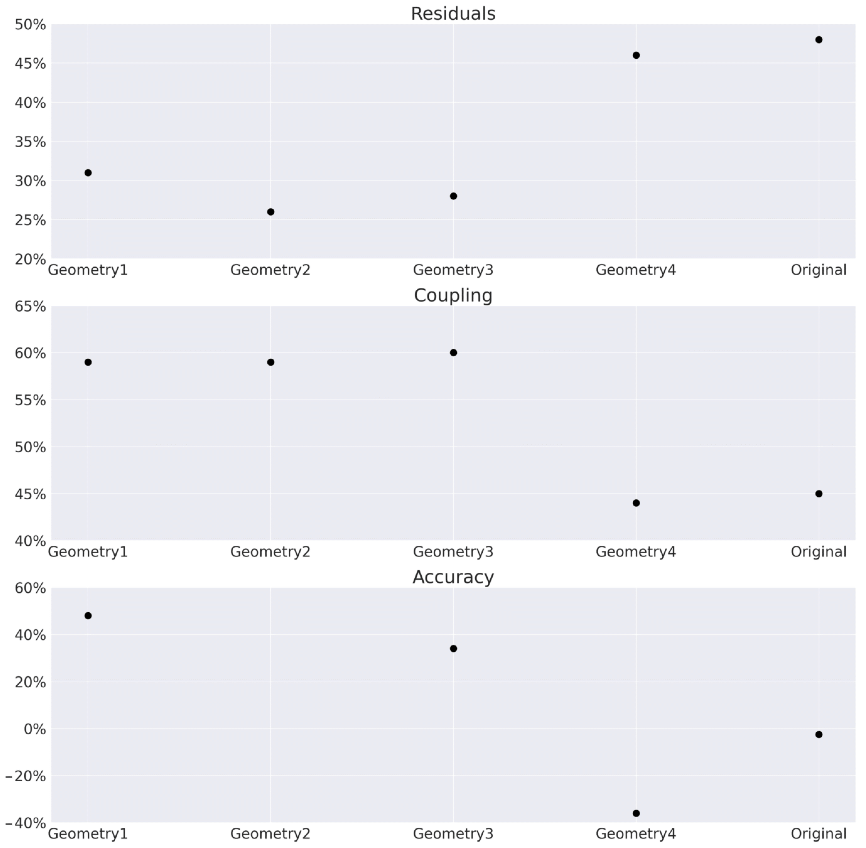
To investigate the optimization methods, as noted, the minimization of hydraulic losses was chosen as the goal function and 100 optimization iterations were allowed for each optimization method. The most appropriate method was chosen based on its ability to provide the best solution in the fewest number of iterations. Although it is possible that with a greater number of iterations (or a larger population) another optimization method could obtain better overall results, it also must be taken into account that optimization problems with computationally expensive function evaluations are difficult to investigate/validate due to computational resource constraints. In other words, our assessment effectively assumes that the optimization method that has a faster convergence at the beginning is more beneficial/effective for the problem in question.

According to our findings, the standard PSO method produced the best results in the shortest number of iterations. However, due to the stochastic nature of the optimization, not all runs with a population size of 20 were able to obtain the same local optima. When the swarm size was increased to 30 or 40, the best solution was obtained in all conducted runs. Therefore, it can be concluded that no notable advantage can be obtained by further increasing the population size. Since one of the goals was to reduce the computational requirements, the PSO method with a population size of 30 was adopted for further optimizations.

3.3. Goal Functions

The optimization workflow using a velocity profile at the inlet, i.e., case 2 with full geometry, was conducted with the PSO algorithm, where the swarm size was set to 30 and in total, 500 iterations were conducted. The remaining parameters were kept the same as in Table 7. Four different optimizations were conducted, as described in Table 5. A visual representation of the obtained results is given in Figure 4. An example of the convergence graphs is given in Figure A1 in Appendix A. It can be seen that the shape for case $O_1$ corresponded to a local optimum; hence, the optimization process was allowed to continue to obtain an improved, feasible shape. For cases where the new design must adhere to the limits of the original shape, similar results were obtained, as seen for both cases $O_2$ and $O_4$. The reduction in the cross-sections can be observed at the beginning, followed by a maximum cross-section at the same location (1–2 m downstream of the center along the x-axis). After that, a reduction in the cross-section width was observed for both cases. The variations in the shape were due to the different goal functions.

The obtained optimal shapes, except for the shape in case $O_1$, which was not a feasible solution, were used for the simulations of the whole turbine. The computational domains are presented in Figure A2 in Appendix B. Second-order accurate schemes were employed for the whole turbine simulation, as in [27], where validation was performed by comparing the results with the in situ measurements. The simulations were steady state and conducted using the frozen-rotor approach. The contours of the velocity magnitude are presented in Figure 5 for several draft tube cross-sections and are augmented with pathlines colored with the velocity magnitudes. Additionally, the static pressure at the runner walls is given using a different color map. A detailed visualization of the fluid flow in the draft tube for the considered shapes is given in Appendix C in Figure A3, Figure A4 and Figure A5. For each simulation, both the $C_d$ improvement (loss reduction) and $C_p$ improvement (pressure recovery increase) were evaluated. The results are presented in

Table 8. Improvements for different optimization goal functions and bounds.

Case	Improvement
	${\mathit{C}}_{\mathit{p}}$	${\mathit{C}}_{\mathit{d}}$
$O_1$	-
$O_2$	5.4%	15.3%
$O_3$	7%	17.2%
$O_4$	8.2%	17.5%

. It can be observed that both the greatest increase in the $C_p$ value and the greatest reduction in the $C_d$ value were obtained for case $O_4$, where the $C_d$ value was considered as a goal function and excavation was not allowed. When the $C_p$ value was used as the goal function under the same limits (case $O_2$), smaller improvements were observed than in the case of the $C_d$ value as the goal function. This indicates that different goal functions can influence the optimization convergence speed. However, this disparity can also be due to the stochastic nature of the optimization; therefore, this should be further explored.

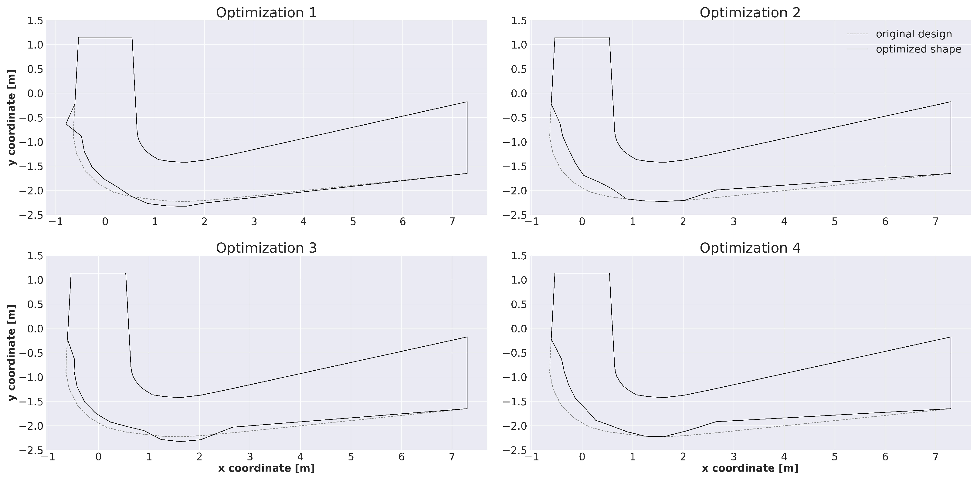
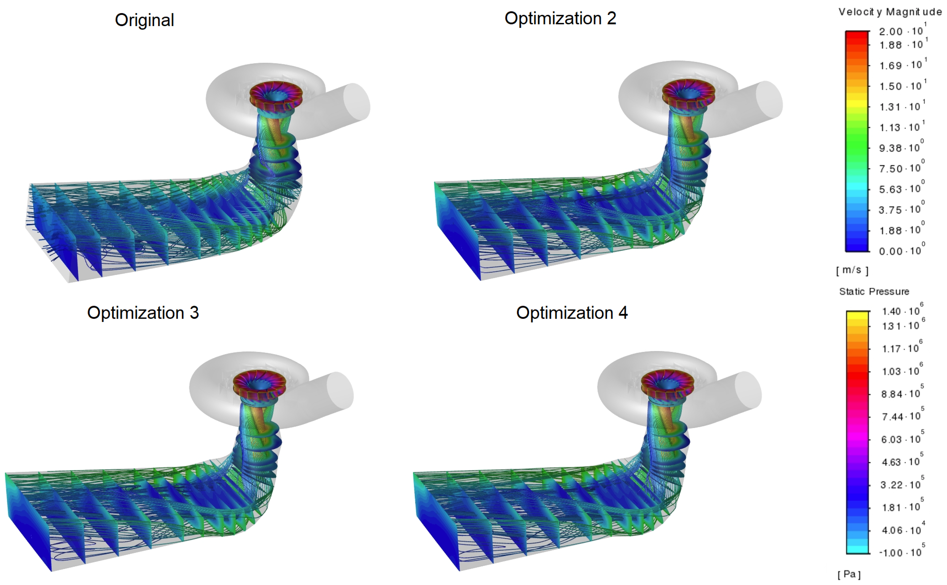
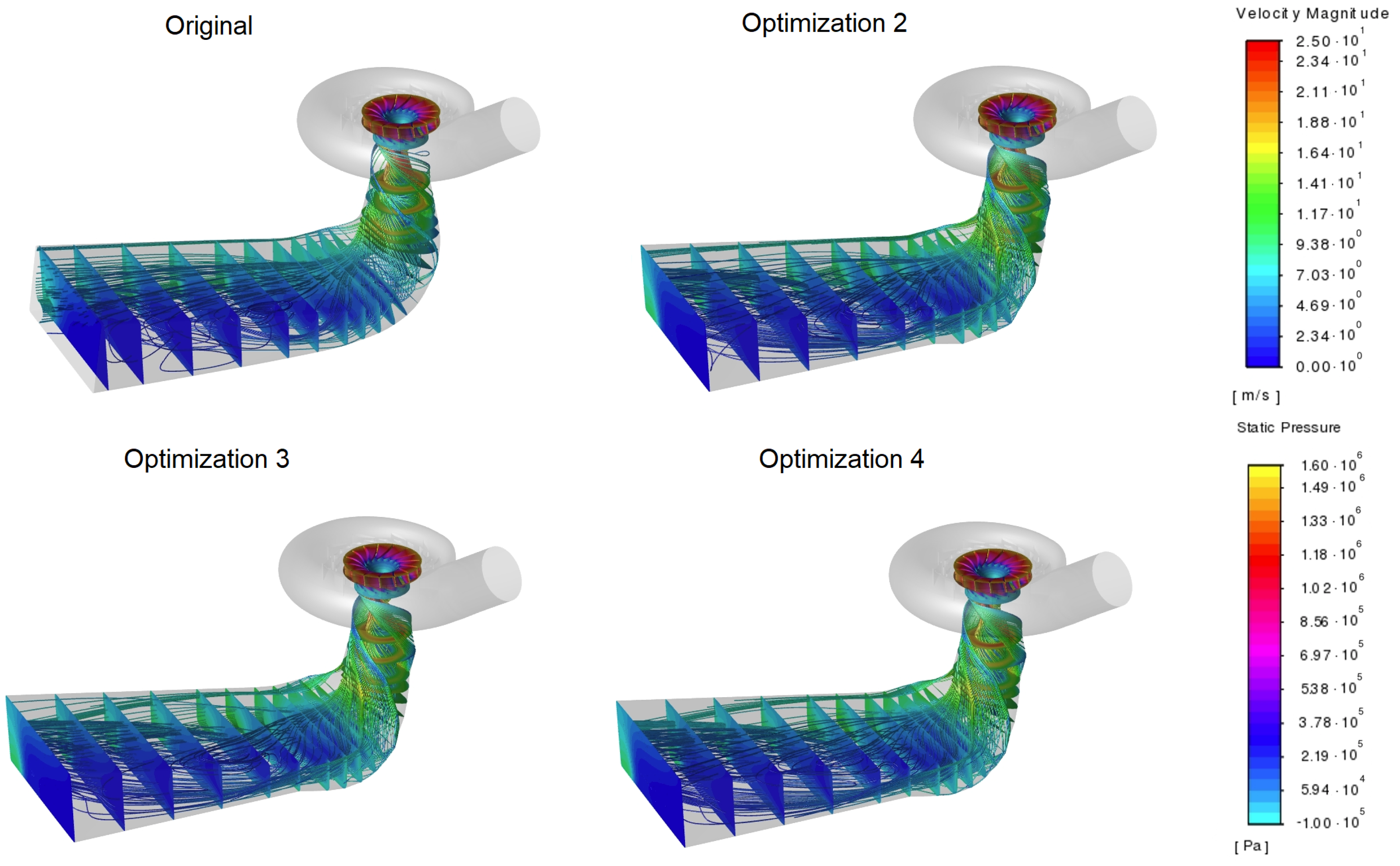
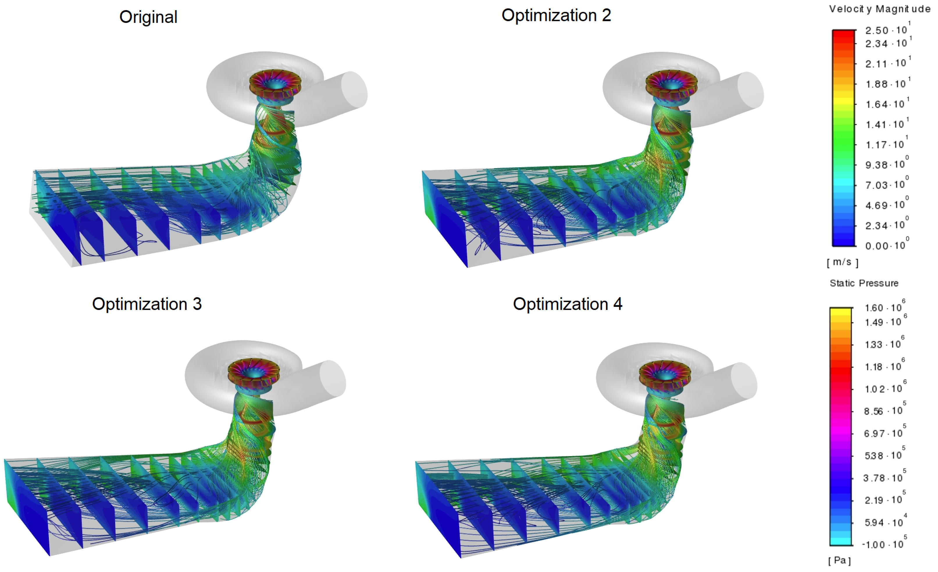
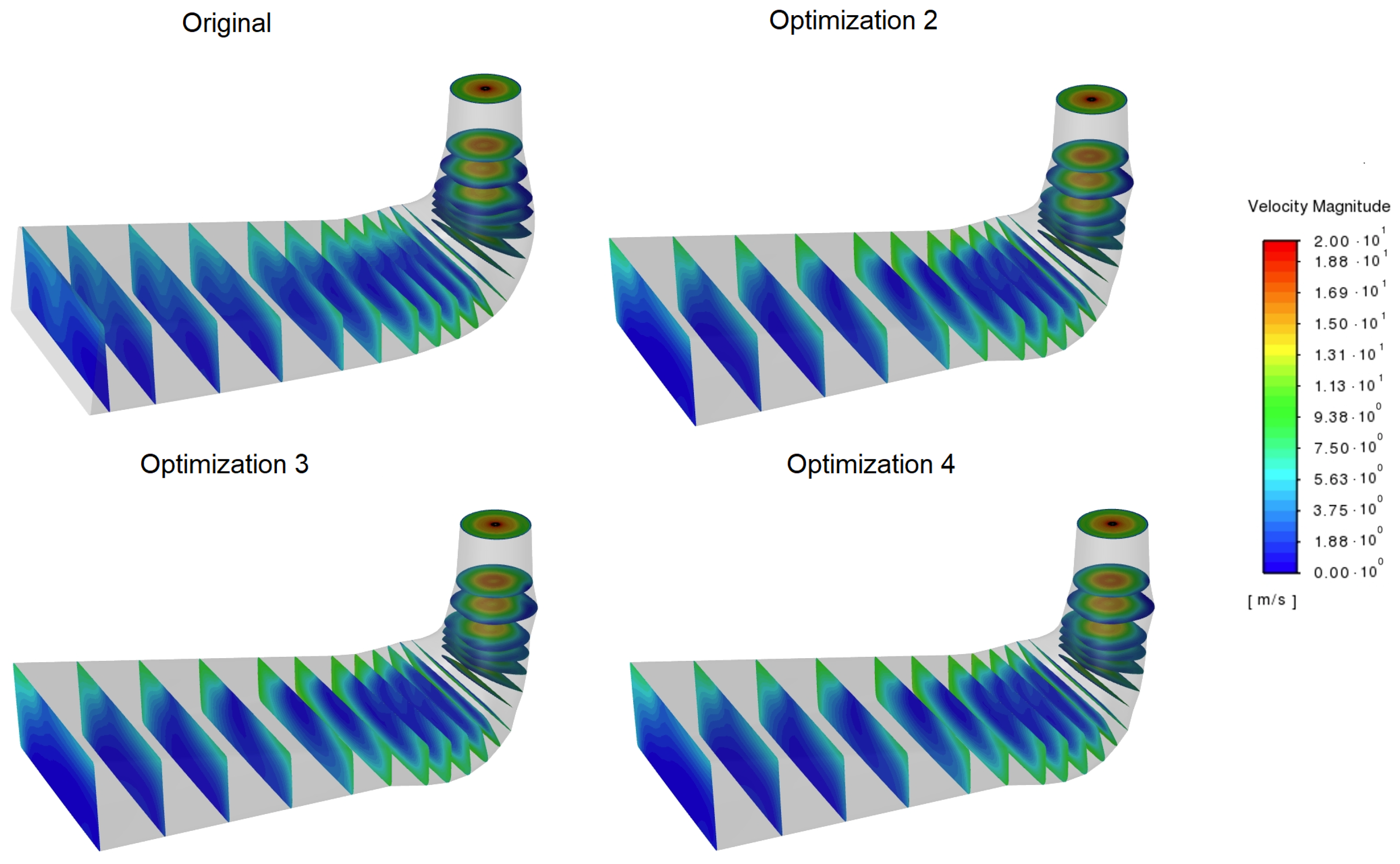
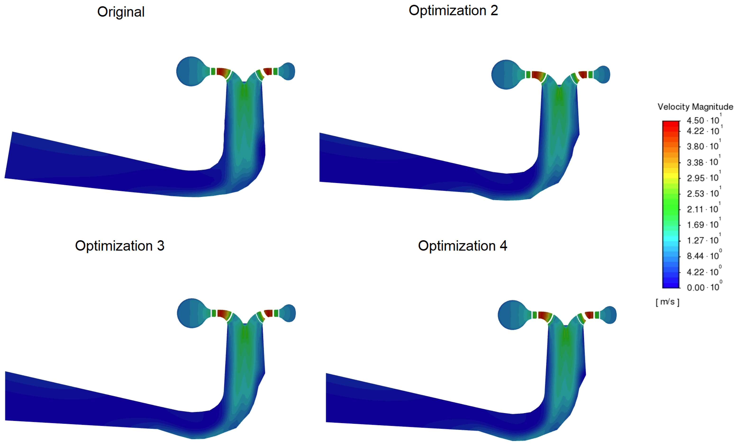
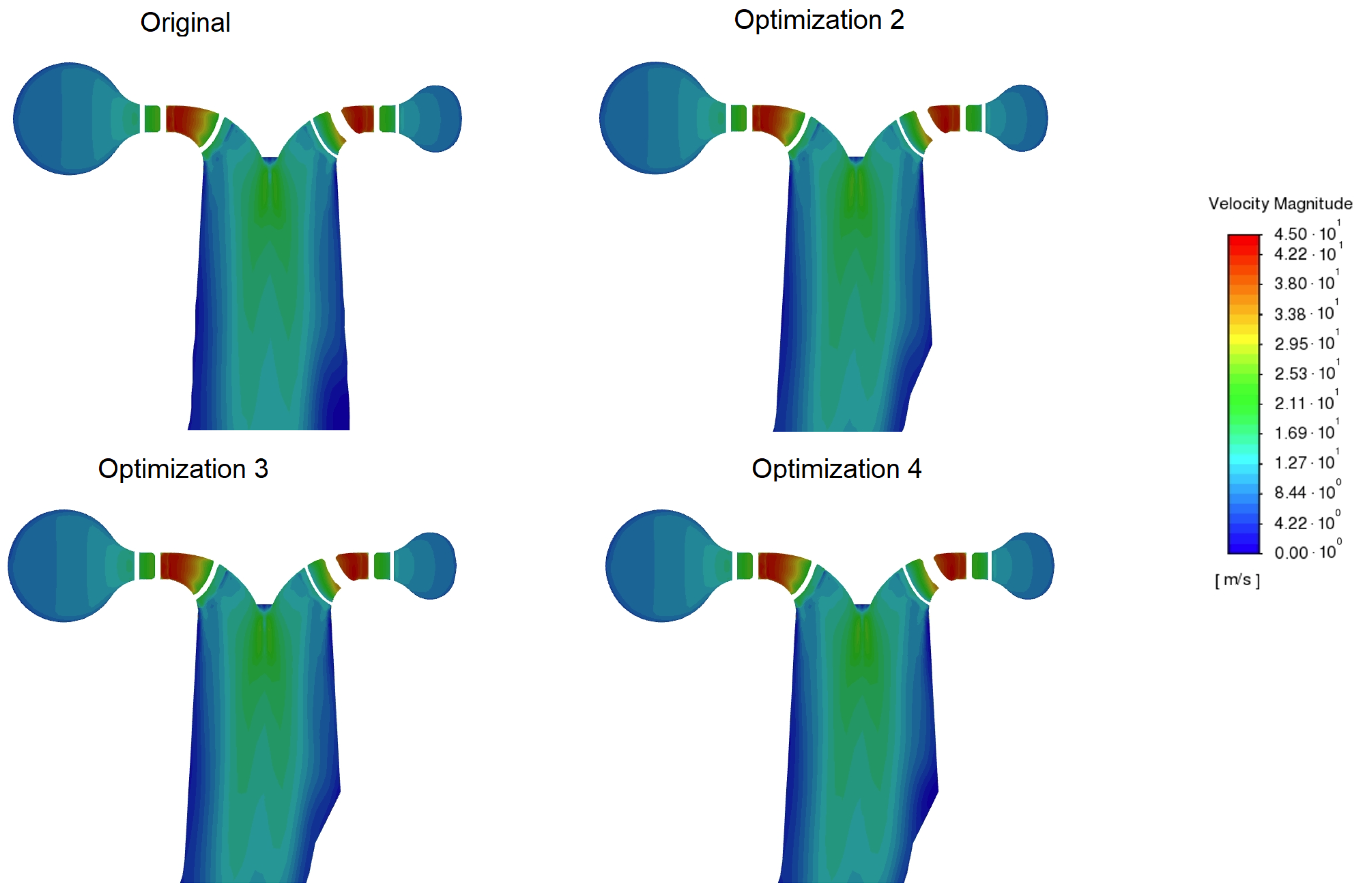
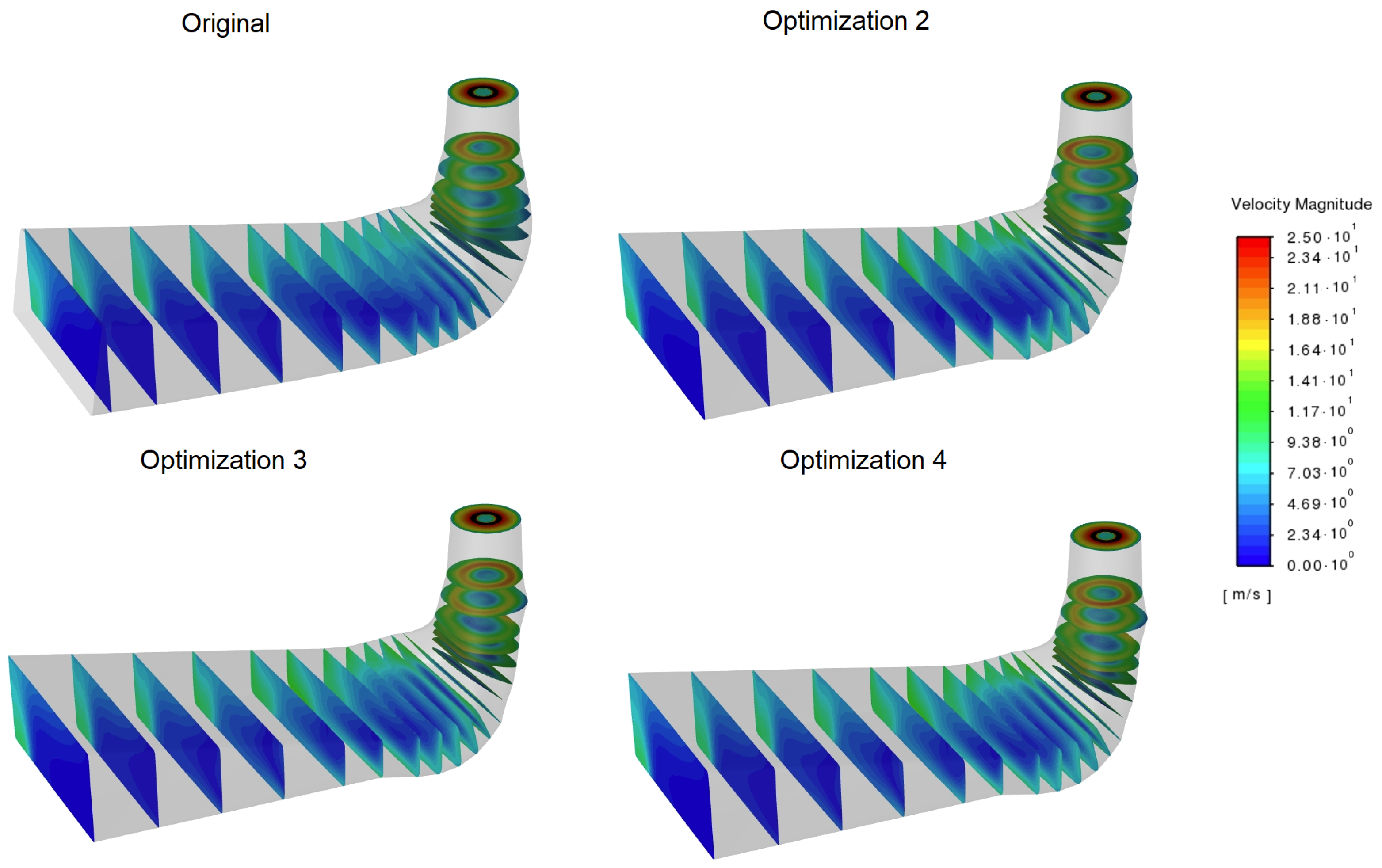
3.4. Optimized Shapes under Various Operating Conditions

Considering that the new draft tube shape should be used under a variety of operating conditions, an additional investigation into optimal shapes was conducted for different volume flow rates. The results are given in

Table 9. Geometry improvements for different flow rates.

Flow Rate	Case	Improvement
		${\mathit{C}}_{\mathit{p}}$	${\mathit{C}}_{\mathit{d}}$
12.8 m${}^3$/s	$O_1$	-
	$O_2$	−4.9%	−4.5%
	$O_3$	−6.2%	−6.7%
	$O_4$	−5.1%	−5.1%
14.3 m${}^3$/s	$O_1$	-
	$O_2$	−9.2%	−7.1%
	$O_3$	−9%	−7.9%
	$O_4$	−9.5%	−8.2%

and shown in Figure 6 and Figure 7. A detailed visualization of the fluid flow in the draft tube for these shapes is given in Appendix C in Figure A6, Figure A7, Figure A8, Figure A9, Figure A10 and Figure A11. It is evident that under different operating conditions, the obtained shapes typically behaved worse than the original draft tube design. This indicates that a multiobjective optimization approach that integrates multiple goal functions, i.e., the maximization of the $C_p$ value at different flow rates, should be considered for the given problem, especially if the turbine often operates outside of the optimal operating point.

4. Discussion

Numerical and optimization parameters that provide a balance of accuracy, robustness, and computational efficiency were investigated in this study. The employed simplifications were validated by performing higher-order numerical analyses in which the obtained optimal draft tube designs were integrated into the turbine, meshed using a structured mesh, and evaluated using steady-state simulations for different flow rates. The results indicate that the proposed designs indeed provide better performance than the initial design; therefore, using numerical simplifications can be considered a valid approach for draft tube optimization. Such an evaluation of the numerical settings for stochastic optimizations has not been previously made in the literature since optimization methods have always been computationally too demanding.

In all cases, the draft tube elbow for the obtained optimal design was moved downstream toward the draft tube outlet. This is a reasonable solution since it enables a smoother flow transition toward the exit. In the work by Daniels et al. [33], a Kaplan draft tube was analyzed and it was noted that the heel of the draft tube had a notable impact on the pressure recovery. Additionally, a reduction in the cross-section in the elbow can be observed in papers by Nakamura and Kurosawa [34] and Lyutov et al. [21], which suggests that similar trends have been previously observed in the literature. It should be noted that the shapes obtained in this study could not be obtained using standard optimization parametrization because the elbow location cannot move in a horizontal direction. However, it must also be noted that the width and upper profile of the draft tube remained constant; therefore, they should be considered in future assessments to determine if the elbow shift can be mitigated by changing other characteristic dimensions.

The overall shape of the optimized design was not smooth, indicating that further improvements to the design can be obtained. In future analyses, geometry parametrization with additional constraints, which would bound the variables to have smaller transitions between the cross-sections, can be used to allow only smooth curves. Another approach is B-splines, with curve parameters as the optimization variables. If the number of optimization parameters defining the B-spline is lower than the number of cross-sections, that approach can also reduce the complexity of the optimization problem. This approach will be investigated in future work. The parametrization flexibility should be carefully investigated and implemented. In Fleischli et al. [19], due to the allowed geometry flexibility, the proposed improved Kaplan draft tube shape had complex smooth surfaces, which are demanding to manufacture.

In terms of numerical accuracy and simulation validity, several assumptions and simplifications were made to reduce the computational time. Although imperfect, this approach allowed for the quick computations needed for the proposed optimization procedure. Certainly, by forcing higher-order schemes or by lowering the y+ value near the wall to better capture the flow, slight improvements in the results might be obtained. From an engineering standpoint, however, this discrepancy should be acceptable. Another issue is the propagation of changes throughout the turbine when considering the different draft tube designs, which might influence the overall flow and the final results. A potential avenue of improvement could be the use of machine learning to lessen the computational load, where trained machine-learning meta-models might be an effective alternative and solution for extensive and complex multiobjective optimizations.

In terms of the optimization procedure, it was discovered that the standard PSO method with a limited number of iterations outperformed the other considered metaheuristic algorithms. It should be noted that if a greater number of iterations and swarm sizes had been allowed and the optimization parameters had been tuned, the other optimization methods might have outperformed the standard PSO, which should be investigated in future work. We have demonstrated that variable boundaries and goal functions can influence the shape of the optimal design. In Favrel et al. [15], it was noted that the energy losses and pressure fluctuation amplitudes as goal functions did not lead to the same set of geometrical parameters. Therefore, appropriate goal function selection needs to be made. In a paper by Lyutov et al. [21], it was noted that when the outlet cross-section was kept constant, the same optimal shape should be expected for both the $C_p$ and $C_d$ goal functions. Similar results were observed in this study. Finally, it can be concluded that the appropriate pick of the goal function can influence the optimization algorithm’s performance, which is exacerbated when only a limited number of optimization iterations are permitted, as was the case in this study.

Additional validation of the obtained optimal designs indicated that the obtained improvements were only valid for the considered operating conditions, whereas in the other cases, worse performance was observed. Since turbines must be designed to operate in a wide operational range, a multiobjective approach should be used in further studies, with multiple operating conditions considered to obtain improved designs for realistic use. Some examples are the draft tube optimization by Lyutov et al. [21] and the runner multiobjective shape optimization by Chirkov et al. [35].

It should also be noted that fluid flow in a draft tube can have considerable pressure pulsations, which can cause cavitation; hence, the use of a steady-state approach was not appropriate for the evaluation of the considered phenomena. Optimizations with unsteady simulations would require an unfeasible amount of time and therefore were not an option. Pressure pulsations were evaluated by Favrel et al. [15]; however, the DoE and ANOM methods were used due to the considerable time and resources needed for unsteady simulations. Still, these phenomena can be evaluated at the end of the optimization procedure to further validate the obtained optimal design. Ultimately, model tests of optimal shapes can be conducted, as in Flores et al. [8], to further validate the obtained designs.

Based on all these observations, it must be emphasized that the obtained draft tube geometries are not as practical. Additional validation with respect to cavitation inception and propagation should also be conducted in order to determine whether the designs are appropriate for real-world use. Smoother curves (and designs) should be obtained with improved parametrization approaches. Additionally, construction, production, and economic aspects should be taken into account.

5. Conclusions

With an increasing demand for renewable energy sources, it is reasonable to assume that a great focus will be given to the development of highly efficient hydro turbines. As computational capabilities increase, the optimization approach for the development of new or the revitalization of old turbines presents an interesting solution. The research conducted in this study provides an extensive investigation of the numerical parameters that are chosen to provide fast and robust optimization execution with the appropriate accuracy. The validation of the simulations of a whole turbine operation, where the obtained optimal draft tube designs were included, further validated the proposed approach. The presented findings provide guidelines for future optimization applications for draft tube improvements.

The fundamental problem with the considered optimization methodology is the expensive fitness function evaluations, thus limiting the extensive optimization parameter investigation. It was observed that the standard PSO method can be successfully used to obtain an improved draft tube design within a limited number of iterations. Based on the obtained optimized designs, the proposed optimization approach enables more flexibility regarding the optimal shape since the lowest point of the draft tube has shifted toward the outlet. However, the proposed parametrization based on cross-section heights needs to be improved since sharp edges were observed in the final geometry. To tackle this issue, spline parameterization needs to be investigated in future works to ensure a smooth shape. Additionally, it was observed that multiobjective optimization should be considered, specifically with multiple operating conditions since the performance of the obtained optimal designs decreased for the other operating conditions.

References

1. Gaudard, L.; Romerio, F. The future of hydropower in Europe: Interconnecting climate, markets and policies. Environ. Sci. Policy 2014, 37, 172–181. [Google Scholar] [CrossRef]
2. Chae, K.J.; Kang, J. Estimating the energy independence of a municipal wastewater treatment plant incorporating green energy resources. Energy Convers. Manag. 2013, 75, 664–672. [Google Scholar] [CrossRef]
3. Chae, K.J.; Kim, I.S.; Ren, X.; Cheon, K.H. Reliable energy recovery in an existing municipal wastewater treatment plant with a flow-variable micro-hydropower system. Energy Convers. Manag. 2015, 101, 681–688. [Google Scholar] [CrossRef]
4. Hunt, J.D.; Zakeri, B.; Lopes, R.; Barbosa, P.S.F.; Nascimento, A.; de Castro, N.J.; Brandão, R.; Schneider, P.S.; Wada, Y. Existing and new arrangements of pumped-hydro storage plants. Renew. Sustain. Energy Rev. 2020, 129, 109914. [Google Scholar] [CrossRef]
5. Liu, X.; Luo, Y.; Karney, B.W.; Wang, W. A selected literature review of efficiency improvements in hydraulic turbines. Renew. Sustain. Energy Rev. 2015, 51, 18–28. [Google Scholar] [CrossRef]
6. Trivedi, C.; Cervantes, M.J.; Gunnar Dahlhaug, O. Numerical techniques applied to hydraulic turbines: A perspective review. Appl. Mech. Rev. 2016, 68, 010802. [Google Scholar] [CrossRef]
7. Tiwari, G.; Kumar, J.; Prasad, V.; Patel, V.K. Utility of CFD in the design and performance analysis of hydraulic turbines—A review. Energy Rep. 2020, 6, 2410–2429. [Google Scholar] [CrossRef]
8. Flores, E.; Bornard, L.; Tomas, L.; Liu, J.; Couston, M. Design of large Francis turbine using optimal methods. In IOP Conference Series: Earth and Environmental Science; IOP Publishing: Bristol, UK, 2012; Volume 15, p. 022023. [Google Scholar]
9. Abbas, A.; Kumar, A. Development of draft tube in hydro-turbine: A review. Int. J. Ambient Energy 2017, 38, 323–330. [Google Scholar] [CrossRef]
10. Sosa, J.; Urquiza, G.; García, J.; Castro, L. Computational fluid dynamics simulation and geometric design of hydraulic turbine draft tube. Adv. Mech. Eng. 2015, 7, 1687814015606307. [Google Scholar] [CrossRef] [Green Version]
11. Amano, R.S.; Abbas, A. Optimization of intake and draft tubes of a Kaplan micro hydro-turbine. In Proceedings of the 15th International Energy Conversion Engineering Conference, Atlanta, GA, USA, 10–12 July 2017; p. 4807. [Google Scholar]
12. Schiffer, J.; Benigni, H.; Jaberg, H. An analysis of the impact of draft tube modifications on the performance of a Kaplan turbine by means of computational fluid dynamics. Proc. Inst. Mech. Eng. Part C J. Mech. Eng. Sci. 2018, 232, 1937–1952. [Google Scholar] [CrossRef]
13. Arispe, T.M.; de Oliveira, W.; Ramirez, R.G. Francis turbine draft tube parameterization and analysis of performance characteristics using CFD techniques. Renew. Energy 2018, 127, 114–124. [Google Scholar] [CrossRef]
14. Chol Nam, M.; Ba, D.; Yue, X.; Jin, M. Design optimization of hydraulic turbine draft tube based on CFD and DOE method. In IOP Conference Series: Earth and Environmental Science; IOP Publishing: Bristol, UK, 2018; Volume 136, p. 012019. [Google Scholar]
15. Favrel, A.; Lee, N.j.; Irie, T.; Miyagawa, K. Design of Experiments Applied to Francis Turbine Draft Tube to Minimize Pressure Pulsations and Energy Losses in Off-Design Conditions. Energies 2021, 14, 3894. [Google Scholar] [CrossRef]
16. Kawajiri, H.; Enomoto, Y.; Kurosawa, S. Design optimization method for Francis turbine. In IOP Conference Series: Earth and Environmental Science; IOP Publishing: Bristol, UK, 2014; Volume 22, p. 012026. [Google Scholar]
17. McNabb, J.; Devals, C.; Kyriacou, S.; Murry, N.; Mullins, B. CFD based draft tube hydraulic design optimization. In IOP Conference Series: Earth and Environmental Science; IOP Publishing: Bristol, UK, 2014; Volume 22, p. 012023. [Google Scholar]
18. Eisinger, R.; Ruprecht, A. Automatic shape optimization of hydro turbine components based on CFD. TASK Q 2002, 6, 101–111. [Google Scholar]
19. Fleischli, B.; Del Rio, A.; Casartelli, E.; Mangani, L.; Mullins, B.; Devals, C.; Melot, M. Application of a General Discrete Adjoint Method for Draft Tube Optimization. In IOP Conference Series: Earth and Environmental Science; IOP Publishing: Bristol, UK, 2021; Volume 774, p. 012012. [Google Scholar]
20. Moravec, P.; Rudolf, P. Application of a particle swarm optimization for shape optimization in hydraulic machinery. EPJ Web Conf. 2017, 143, 02076. [Google Scholar] [CrossRef] [Green Version]
21. Lyutov, A.; Chirkov, D.; Skorospelov, V.; Turuk, P.; Cherny, S. Coupled multipoint shape optimization of runner and draft tube of hydraulic turbines. J. Fluids Eng. 2015, 137. [Google Scholar] [CrossRef]
22. Bonacci, O.; Oštrić, M.; Bonacci, T.R. Water resources analysis of the Rječina karst spring and river (Dinaric karst). Acta Carsol. 2018, 47, 123–137. [Google Scholar] [CrossRef] [Green Version]
23. Skotak, A.; Mikulasek, J.; Obrovsky, J. Development of the new high specific speed fixed blade turbine runner. Int. J. Fluid Mach. Syst. 2009, 2, 392–399. [Google Scholar] [CrossRef] [Green Version]
24. Puente, L.; Reggio, M.; Guibault, F. Automatic shape optimization of a hydraulic turbine draft tube. In Proceedings of the International Conference, CFD2003, Vancouver, BC, Canada, 28–30 May 2003; Volume 28. [Google Scholar]
25. Orso, R.; Benini, E.; Minozzo, M.; Bergamin, R.; Magrini, A. Two-objective optimization of a Kaplan turbine draft tube using a Response Surface Methodology. Energies 2020, 13, 4899. [Google Scholar] [CrossRef]
26. Menter, F.R.; Kuntz, M.; Langtry, R. Ten years of industrial experience with the SST turbulence model. Turbul. Heat Mass Transf. 2003, 4, 625–632. [Google Scholar]
27. Čarija, Z.; Mrša, Z.; Fućak, S. Validation of Francis water turbine CFD simulations. Stroj. Časopis Teor. Praksu Stroj. 2008, 50, 5–14. [Google Scholar]
28. Kennedy, J.; Eberhart, R. Particle swarm optimization. In Proceedings of the ICNN’95-International Conference on Neural Networks, Perth, Australia, 27 November–1 December 1995; Volume 4, pp. 1942–1948. [Google Scholar]
29. Tan, Y.; Zhu, Y. Fireworks algorithm for optimization. In Proceedings of the International Conference in Swarm Intelligence, Beijing, China, 12–15 June 2010; pp. 355–364. [Google Scholar]
30. Jain, M.; Singh, V.; Rani, A. A novel nature-inspired algorithm for optimization: Squirrel search algorithm. Swarm Evol. Comput. 2019, 44, 148–175. [Google Scholar] [CrossRef]
31. Tanabe, R.; Fukunaga, A.S. Improving the search performance of SHADE using linear population size reduction. In Proceedings of the 2014 IEEE congress on evolutionary computation (CEC), Beijing, China, 6–11 July 2014; pp. 1658–1665. [Google Scholar]
32. Družeta, S.; Ivić, S. Indago—Python Module for Numerical Optimization. Available online: https://pypi.org/project/Indago/ (accessed on 12 January 2022).
33. Daniels, S.; Rahat, A.; Tabor, G.; Fieldsend, J.; Everson, R. Shape optimisation of the sharp-heeled Kaplan draft tube: Performance evaluation using Computational Fluid Dynamics. Renew. Energy 2020, 160, 112–126. [Google Scholar] [CrossRef]
34. Nakamura, K.; Kurosawa, S. Design optimization of a high specific speed Francis turbine using multi-objective genetic algorithm. Int. J. Fluid Mach. Syst. 2009, 2, 102–109. [Google Scholar] [CrossRef]
35. Chirkov, D.V.; Ankudinova, A.S.; Kryukov, A.E.; Cherny, S.G.; Skorospelov, V.A. Multi-objective shape optimization of a hydraulic turbine runner using efficiency, strength and weight criteria. Struct. Multidiscip. Optim. 2018, 58, 627–640. [Google Scholar] [CrossRef]
Figure 1. Draft tube used for the optimization with different cross-sections.
Mathematics 10 04050 g001
Figure 2. Draft tube with indicated geometry parameters.
Mathematics 10 04050 g002
Figure 3. Relative reduction in number of needed iterations for satisfying convergence criteria for different numerical parameter settings.
Mathematics 10 04050 g003
Figure 4. Overlapping visualization of original geometry and optimized shapes for different optimization goal functions and variable constraints. In the first column, additional excavation was allowed and in the second column, no excavation was allowed.
Mathematics 10 04050 g004
Figure 5. Runner colored to show static pressure and the contours of the velocity magnitudes in several draft tube cross-sections, with the pathlines starting from the runner outlet.
Mathematics 10 04050 g005
Figure 6. Runner colored to show the static pressure value and the contours of the velocity magnitudes in several draft tube cross-sections, with pathlines starting from the runner outlet for an inlet volume flow rate of 12.8 m 3 /s.
Mathematics 10 04050 g006
Figure 7. Runner colored to show static pressure value and the contours of the velocity magnitudes in several draft tube cross-sections, with pathlines starting from the runner outlet for an inlet volume flow rate of 14.3 m 3 /s.
Mathematics 10 04050 g007