Fractional Systems’ Identification Based on Implicit Modulating Functions

Abstract

This paper presents a new method for parameter identification based on the modulating function method for commensurable fractional-order models. The novelty of the method lies in the automatic determination of a specific modulating function by controlling a model-based auxiliary system, instead of applying and parameterizing a generic modulating function. The input signal of the model-based auxiliary system used to determine the modulating function is designed such that a separate identification of each individual parameter of the fractional-order model is enabled. This eliminates the shortcomings of the common modulating function method in which a modulating function must be adapted to the investigated system heuristically.

1. Introduction

Fractional calculus is derived from the field of mathematics and the research on this field is still ongoing [1,2]. In recent years, fractional calculus is being used more and more in the engineering field. Complex physical, chemical e.g., Lithium-ion batteries [3], or biological systems e.g., blood alcohol model [4] are increasingly being described by fractional-order models. Fractional differential equations are also used to describe parts of electrical circuits or refine the description of friction equations in mechanical systems. An overview of technical areas is provided by [5]. Due to the non-locality and memory of fractional integration and differentiation, these models approximate partial differential equations more accurately than classic integer-order models [6]. Over the last years, identification methods considering fractional-order models based on the modulating function method (see e.g., [7,8,9,10,11,12,13,14]) have become more prevalent. A benefit of the modulating function method is that a system of algebraic equations may be solved for the parameter identification instead of a set of differential equations and the measured signal need not be differentiated [15]. In current approaches, a generic modulating function is chosen and parameterized heuristically. This procedure constitutes time-consuming educated guessing which does not generalize or provide clues for new applications, especially in the fractional order case. Thus, parameterizing the modulating function is a significant shortcoming of this method. For parameter identification, the algebraic equations are collected in a linear system which has to be solved. Because the modulating function is chosen and parameterized a-priori, linear dependencies between the individual algebraic equations can occur, depending on the measured signal. In this case, the parameter identification cannot be performed, which constitutes is a significant shortcoming of this method.

In this paper, we propose a systematic procedure for parameter identification using an implicit determination of a modulating function considering the current measurements. This procedure allows for direct parameter identification, without requiring the explicit calculation of modulating function. To the best of the authors’ knowledge, it is the first time that a method that automatically determines a modulating function for the parameter identification of a fractional-order model is presented. While this idea has been described for integer-order models [16], this result does not easily generalize to the non-integer order case.

The paper is structured as follows: In Section 2, the basics of fractional calculus are provided. In Section 3, the modulating function method is recapped and an additional property for the modulating function method, enabling the separate identification of the parameters, are given. Afterward, the model-based auxiliary system, which is central in determining a modulating function automatically, is derived in Section 4. The model-based auxiliary system is used to transfer the heuristic determination of a modulating function into a control problem which allows an automatic determination of the parameter-specific modulating function. A solution to the control problem is provided in Section 5, which leads to the parameter identification and represents the main contribution of this paper. Additionally, the error occurs due to superposed noise on the input and output signal is analyzed. A numerical example in Section 6 demonstrating the efficacy of the proposed algorithm concludes the paper.

2. Preliminaries

2.1. Fundamentals of Fractional Calculus

Throughout this paper, consider the smooth functions $f:(-\infty ,t]\to \mathbb{R}$ and $h:[t,\infty )\to \mathbb{R}$ with the properties $f\left(t\right)=0,\forall t\le t_0$ and $h\left(t\right)=0,\forall t\ge t_e$. Let $\alpha \in {\mathbb{R}}_{>0}$ and $t_0\le t_1<t<t_2\le t_e$ hold. Furthermore, $\lfloor ·\rfloor$ describes the floor function and denotes the biggest integer smaller or equal to the argument and is used to state a modified ceiling-function $\lceil ·\rceil :=\lfloor ·\rfloor +1$. The functions f and h are assumed to be Lebesgue integrable on the integration interval defined by $\left[t_0,t_e\right]$ (see [17]). In addition, the assumption is made that f and h are $\lceil \alpha \rceil$-times absolutely continuous on the derivation interval $\left[t_0,t_e\right]$, where $\alpha$ is the derivation order (see [17]).

Remark 1. 

With regard to the parameter identification, the time variables $t_0$, $t_1$, $t_2$, $t_e$, and t are interpreted as follows. While $t_0$ describes the point of time before the system is at rest, $t_e$ describes the point of time after the system is at rest. The time variable $t_1$ marks the beginning of the identification, $t_2$ notes the end of the identification, and t is the independent integration variable.

The uninitialized as well as initialized fractional operators are described in [18] and are given in the following definition. The initialized fractional operators consist of the uninitialized fractional operator and time-variant initialization functions $\eta :{\mathbb{R}}^5\to \mathbb{R}$ or $\psi :{\mathbb{R}}^5\to \mathbb{R}$, which have been proven to be necessary in order to describe fractional differential equations (FDEs) correctly. Differing from the notation used in [18], in this paper, an additional operator index on the top left of the fractional operator is used (see [19]). This index indicates that the function is integrated or differentiated w.r.t. the named variable. The index on the bottom left represents the lower bound of the fractional integral and the index on the bottom right is the upper bound. The order of the integration or derivative is given by the top right index. The calculus of two-variable functions can be directly extended from the fractional operators for functions depending on one variable (see [20]).

In the following definition, the uninitialized and the initialized fractional integration along with the Riemann-Liouville ($RL$) and the Caputo (C) fractional derivatives according to [21] are summarized.

Definition 1. (Fractional Operators.) 

• Uninitialized Fractional Integral

  $${}_{t_0}{}^{\tau }i_t^{\alpha }f\left(\tau \right):=\frac{1}{\Gamma \left(\alpha \right)}{\int }_{t_0}^t\frac{f\left(\nu \right)}{{(t-\nu )}^{(1-\alpha )}}\mathrm{d}\nu$$

  (1)
• Initialized Fractional Integral

  $${}_{t_1}{}^{\tau }\mathcal{I}_t^{\alpha }f\left(\tau \right):={}_{t_1}{}^{t}i_t^{\alpha }f\left(t\right)+\eta \left(f,\alpha ,t_0,t_1,t\right)$$

  (2)
• Uninitialized Riemann-Liouville Fractional Derivative

  $${}_{t_0}{}^{\tau }\mathrm{d}RL_t^{\alpha }f\left(\tau \right):={\left(\frac{\mathrm{d}}{\mathrm{d}t}\right)}^{\lceil \alpha \rceil }\left[{}_{t_0}{}^{\tau }i_t^{\lceil \alpha \rceil -\alpha }f\left(\tau \right)\right]$$

  (3)
• Uninitialized Caputo Fractional Derivative

  $${}_{t_0}{}^{\tau }\mathrm{d}C_t^{\alpha }f\left(\tau \right):={}_{t_0}{}^{\tau }i_t^{\lceil \alpha \rceil -\alpha }\left[{\left(\frac{\mathrm{d}}{\mathrm{d}\tau }\right)}^{\lceil \alpha \rceil }f\left(\tau \right)\right]$$

  (4)
• Initialized Fractional Derivative

  $${}_{t_1}{}^{\tau }\mathrm{D}_t^{\alpha }f\left(\tau \right):={}_{t_1}{}^{\tau }\mathrm{d}_t^{\alpha }f\left(\tau \right)+\psi \left(f,\alpha ,t_0,t_1,t\right)$$

  (5)

where Γ is the Gamma function (see [22] (pp. 1–6)).

Remark 2. 

The definition of the Riemann-Liouville (3) and the Caputo (4) fractional derivative are connected by

$${}_{t_0}{}^{\tau }\mathrm{d}RL_t^{\alpha }f\left(\tau \right)={}_{t_0}{}^{\tau }\mathrm{d}C_t^{\alpha }f\left(\tau \right)+{\displaystyle \sum _{k=0}^{\lfloor \alpha \rfloor }}{}_{t_0}{}^{\tau }\mathrm{d}RL_t^{\alpha }{\left.\frac{f^{\left(k\right)}\left(\tau \right)}{k!}\right|}_{\tau =t_0}{\left(t-t_0\right)}^k$$

(6)

which is given in [17].

Remark 3. 

In (2) and in (5), the application of the initialization function η or ψ necessitates knowledge of the function f in the interval $t\in \left[t_0,t_1\right]$ (see [18]). To ensure that a system is at rest, the initialization function implies that f has to be known from $t_0\to -\infty$ according to [18]. Therefore, an exact initialization is not possible in practical applications.

Remark 4. 

In (5), the specific operator depends on the utilized uninitialized operator (3) or (4). Thus, ${}_{t_1}{}^t\mathrm{D}_t^{\alpha }f\left(t\right)$ may be described by either ${}_{t_1}{}^t\mathrm{D}RL_t^{\alpha }$ or ${}_{t_1}{}^t\mathrm{D}C_t^{\alpha }$ and must correspond to the uninitialized operator (see [18]). According to the uninitialized operator, the related initialization function has to be employed (see [18]).

In addition to the left-sided definitions, the equivalent right-sided definitions of the integrations (1) and (2) and derivatives (3)–(5) exist.

Definition 2. (Uninitialized Right-Sided Fractional Integral.)

$${}_t{}^{\tau }i_{t_e}^{\alpha }h\left(\tau \right):=\frac{1}{\Gamma \left(\alpha \right)}{\int }_t^{t_e}\frac{h\left(\nu \right)}{{(\nu -t)}^{(1-\alpha )}}\mathrm{d}\nu .$$

(7)

The other definitions follow directly by inserting (7) instead of (1) into the definitions (2)–(5). These are explicitly given in Appendix A. The left- and right-sided fractional operators are connected by a reflection operator $\mathbb{Q}$.

Definition 3. (Reflection Operator.)

The reflection operator $\mathbb{Q}$ maps a left-sided function f onto a right-sided one $\tilde{f}$ (see [23]):

$$\mathbb{Q}f\left(t\right):=f\left(t_1+t_2-t\right)=\tilde{f}\left(t\right).$$

(8)

2.2. Fractional-Order Models

We define the commensurable fractional-order model using the initialized Caputo fractional derivative (5)

$${}_t{}^t\mathrm{D}C_{t_2}^{n\alpha }{\tilde{y}}_o\left(t\right)+\sum _{i=0}^{n-1}{a}_i{}_t{}^t\mathrm{D}C_{t_2}^{i\alpha }{\tilde{y}}_o\left(t\right)=\sum _{j=0}^m{b}_j{}_t{}^t\mathrm{D}C_{t_2}^{j\alpha }{\tilde{u}}_o\left(t\right)$$

(9)

where $a_i$, $b_j\in \mathbb{R}$ are unknown parameters. The number of parameters $n,m\in {\mathbb{N}}_{\ge 0}$ can either be determined by white-box modeling or be specified for black-box modeling. We thus assume n and m are known. The fractional order $\alpha \in {\mathbb{R}}_{>0}$ is usually unknown and has to be identified as well.

The input ${\tilde{u}}_o$ and output signal ${\tilde{y}}_o$ in (9) are a noisy observation of the undisturbed input u

$${\tilde{u}}_o\left(t\right)=\tilde{u}\left(t\right)+{\tilde{u}}_e\left(t\right)$$

(10)

and of the undisturbed output y

$${\tilde{y}}_o\left(t\right)=\tilde{y}\left(t\right)+{\tilde{y}}_e\left(t\right),$$

(11)

to which the reflection operator (8) has been applied. The measurement disturbances are represented by ${\tilde{u}}_e$ and ${\tilde{y}}_e$.

Remark 5. 

The reflected signals are used instead of the original signals since this allows a left-sided auxiliary system to be derived (see Section 4).

Regarding the input signal $\tilde{u}$, we assume that the system is persistently excited, which is a necessary condition for parameter identification [24] (p. 250). In Appendix C, we show that the condition of persistent excitation collapses into a necessary condition on the signal $\tilde{u}$ (see Lemma A3).

Assumption A1. (Known Fractional Order.)

In this paper, it is assumed that the order is provided by another method like in [25,26]. From this assumption, it directly follows that the fractional orders are known for parameter identification. Furthermore, we consider stable systems and, because of the extended Matignon’s theorem (see [26]), $\alpha \in (0,2)$ is assumed.

Despite the restrictions placed by Assumption A1, we note that the derivations are not limited solely to this case.

3. Parameter-Specific Identification Using Modulating Function Method

The modulating function method is a well-known method for the parameter identification of fractional-order models (see e.g., [7,8,9,10,11,12]). The modulating function method was derived in [27] for the integer-order case and has been transferred to the fractional-order case (see e.g., [7,8,9,10,11,12]). In Section 3.1, we shortly recap the modulating function approach to introduce the necessary notation. Based on the recap, a parameter-specific modulating function is defined in Section 3.2. The properties of such a parameter-specific modulating function are used to transfer the identification problem into a control problem in Section 5.

3.1. Fractional Modulating Function Method

Suppose, a modulating function $\phi$ exists which fulfills Assumption A2.

Assumption A2. (Properties of Modulating Functions.)

Suppose $\mathcal{J}:=\left\{\left.i\in {\mathbb{N}}_{>0}\right|i\le n\right\}$ and $\mathcal{K}:=\left\{\left.k\in {\mathbb{N}}_{>0}\right|\exists i\in \mathcal{J}:k\le i\lfloor \alpha \rfloor \right\}$. The modulating function $\phi :\mathbb{R}\to \mathbb{R}$ fulfills the properties:

$$\begin{array}{c}\left(P1\right)\phantom{i}:\phantom{i}\phi \left(t\right)\in {\mathcal{C}}^{n\alpha }\left([t_1,t_2]\right),\hfill \\ \left(P2\right)\phantom{i}:\phantom{i}{\left.{\left(\frac{\mathrm{d}}{\mathrm{d}t}\right)}^k\left({}_{t_1}{}^{t}i_t^{\lceil i\alpha \rceil -i\alpha }\phi \left(t\right)\right)\right|}_{t=t_1}={\left.{\left(\frac{\mathrm{d}}{\mathrm{d}t}\right)}^k\left({}_{t_1}{}^{t}i_t^{\lceil i\alpha \rceil -i\alpha }\phi \left(t_2\right)\right)\right|}_{t=t_1}=0\mathrm{and}\hfill \\ \left(P3\right)\phantom{i}:\phantom{i}{}_{t_1}{}^t\mathrm{d}RL_t^{i\alpha }\phi \left(t\right)=0\hfill \end{array}$$

where $\mathcal{C}$ indicates the class of continuously differentiable functions, $i\in \mathcal{J}$, and $k\in \mathcal{K}$.

The property $\left(P3\right)$ ensures that the influence of the initialization function $\psi$ in (9) is eliminated. Multiplying (9) with a modulating function $\phi$ and integrating the resulting equation by parts results in

$$\sum _{i=0}^n{a}_i\underset{t_1}{\overset{t_2}{\int }}{\tilde{y}}_o\left(t\right){}_{t_1}{}^t\mathrm{d}RL_t^{i\alpha }\phi \left(t\right)\mathrm{d}t=\sum _{j=0}^m{b}_j\underset{t_1}{\overset{t_2}{\int }}{\tilde{u}}_o\left(t\right){}_{t_1}{}^t\mathrm{d}RL_t^{j\alpha }\phi \left(t\right)\mathrm{d}t.$$

(12)

without loss of generality we assume $a_n=1$. This results in the well-known lemma for the identification of the unknown parameters (see [12]). Note, the mathematical operations changes the Caputo initialized fractional derivative used in (9) into uninitialized Riemann-Liouville fractional derivative (3) in (12).

Lemma 1. (Parameter Identification Applying Modulating Function Method.)

Suppose $t,t_1\in \mathbb{R}$, $T_{\Delta },T_I\in {\mathbb{R}}_{>0}$, the modulating-function φhas property $\left(P3\right)$, the system

$${}_t{}^t\mathrm{D}C_{t2}^{n\alpha }{\tilde{y}}_o\left(t\right)+\sum _{i=0}^{n-1}{a}_i{}_t{}^t\mathrm{D}C_{t2}^{i\alpha }{\tilde{y}}_o\left(t\right)=\sum _{j=0}^m{b}_j{}_t{}^t\mathrm{D}C_{t2}^{j\alpha }{\tilde{u}}_o\left(t\right),$$

(13)

$h\in {\mathbb{N}}_{\ge 0}$, $h\ge n+m+1$, $\mathcal{L}:=\left\{\left.l\in {\mathbb{N}}_{\ge 0}\right|l\le h\right\}$, $l\in \mathcal{L}$, $t_l=t_1+l{T}_{\Delta }$, and $\mathit{p}:={\left[a_0\cdots a_{n-1}{b}_0\cdots b_m\right]}^{\top }$. Furthermore, suppose $\mathit{M}:={\left[{\mathit{m}}_0\cdots {\mathit{m}}_l\cdots {\mathit{m}}_h\right]}^{\top }$, where ${\mathit{m}}_l$ is given by

$$\begin{array}{cc}\hfill {\mathit{m}}_l^{\top }& :=\left[-\underset{t_l}{\overset{t_l+T_I}{\int }}y\left(t\right)\phi \left(t\right)\mathrm{d}t\cdots -\underset{t_l}{\overset{t_l+T_I}{\int }}y\left(t\right){}_{t_1}{}^t\mathrm{d}RL_t^{(n-1)\alpha }\phi \left(t\right)\mathrm{d}t\right.\hfill \\ \hfill & \left.\underset{t_l}{\overset{t_l+T_I}{\int }}u\left(t\right)\phi \left(t\right)\mathrm{d}t\cdots \underset{t_l}{\overset{t_l+T_I}{\int }}u\left(t\right){}_{t_1}{}^t\mathrm{d}RL_t^{m\alpha }\phi \left(t\right)\mathrm{d}t\right].\hfill \end{array}$$

(14)

Is $\mathit{M}$ regular, we get the parameters out of

$$\mathit{z}=\mathit{M}\mathit{p}$$

(15)

where $\mathit{z}:={\left[z_0\cdots z_l\cdots z_h\right]}^{\top }$ and

$$z_l:=\underset{t_l}{\overset{t_l+T_I}{\int }}y\left(t\right){}_{t_1}{}^t\mathrm{d}RL_t^{n\alpha }\phi \left(t\right)\mathrm{d}t.$$

(16)

Proof. 

The proof can be found in [12]. □

We note that, depending on the a-priori chosen modulating functions and their parameterization, the equations of system (14) can be linearly dependent, which presents an obstacle for the identification of parameters.

3.2. Parameter-Specific Modulating Function

Sometimes, it is favorable to identify just one parameter at a time. Therefore, we introduce a parameter-specific modulation function approach. Suppose ${\mathit{m}}_o\left(t_2\right)={\mathit{e}}_s$ holds true for each parameter $p_s$, where $p_s$ represents the s-th element of the parameter vector $\mathit{p}:={\left[a_0\cdots a_{n-1}{b}_0\cdots b_m\right]}^{\top }$. Call ${\phi }_s$ parameter-specific modulating. In summary, in line with the assumption $\left(P1\right)$–$\left(P3\right)$ we define:

Definition 4. (Parameter-Specific Modulating Function Set.)

Suppose $\mathcal{J}:=\left\{\left.i\in {\mathbb{N}}_{>0}\right|i\le n\right\}$ and $\mathcal{K}:=\left\{\left.k\in {\mathbb{N}}_{>0}\right|\exists i\in \mathcal{J}:k\le \lfloor i\alpha \rfloor \right\}$. The parameter-specific set ${\mathcal{W}}_s$ is defined as follows:

$$\begin{array}{cc}\hfill {\mathcal{W}}_s& :={\mathcal{W}}_1\cap {\mathcal{W}}_2\cap {\mathcal{W}}_3^s\hspace{1em}\hspace{1em}\hspace{1em}\hspace{1em}\hspace{1em}\hspace{1em}\hspace{1em}\hspace{1em}\hspace{1em}\hspace{1em}\hspace{1em}\hspace{1em}\hspace{1em}\hspace{1em}\hspace{1em}\hspace{1em}\hspace{1em}\hspace{1em}\hfill \end{array}$$

(17)

$$\begin{array}{cc}\hfill {\mathcal{W}}_1& :=\left\{\left.{\phi }_s:\mathbb{R}\to \mathbb{R}\right|{\phi }_s\left(t\right)=0\forall t\le t_1\right\}\hspace{1em}\hspace{1em}\hspace{1em}\hspace{1em}\hspace{1em}\hspace{1em}\hspace{1em}\hspace{1em}\hspace{1em}\hspace{1em}\hspace{1em}\hspace{1em}\hfill \end{array}$$

(18)

$$\begin{array}{cc}\hfill {\mathcal{W}}_2& :=\left\{\left.{\phi }_s:\mathbb{R}\to \mathbb{R}\right|\forall i\in \mathcal{J}\wedge \forall k\in \mathcal{K}:{\left.{}_{t_1}{}^t\mathrm{d}RL_t^{i\alpha +k-\lceil i\alpha \rceil }{\phi }_s\left(t\right)\right|}_{t=t_2}=0\right\}\hfill \end{array}$$

(19)

$$\begin{array}{cc}\hfill {\mathcal{W}}_3^s& :=\left\{{\phi }_s:\mathbb{R}\to \mathbb{R}\left|{\mathit{m}}_o\left(t_2\right)={\mathit{e}}_s\right.\right\}\hspace{1em}\hspace{1em}\hspace{1em}\hspace{1em}\hspace{1em}\hspace{1em}\hspace{1em}\hspace{1em}\hspace{1em}\hspace{1em}\hspace{1em}\hspace{1em}\hspace{1em}\hspace{1em}\hfill \end{array}$$

(20)

where the fractional derivative is given in (3), ${\mathit{m}}_o$ is given by

$$\begin{array}{cc}\hfill {\mathbf{m}}_o^{\top }\left(t_2\right)& :=\left[-\underset{t_1}{\overset{t_2}{\int }}{\tilde{y}}_o\left(t\right){\phi }_s\left(t\right)\mathrm{d}t\cdots -\underset{t_1}{\overset{t_2}{\int }}{\tilde{y}}_o\left(t\right){}_{t_1}{}^t\mathrm{d}RL_t^{(n-1)\alpha }{\phi }_s\left(t\right)\mathrm{d}t\right.\hfill \\ \hfill & \left.\underset{t_1}{\overset{t_2}{\int }}{\tilde{u}}_o\left(t\right){\phi }_s\left(t\right)\mathrm{d}t\cdots \underset{t_1}{\overset{t_2}{\int }}{\tilde{u}}_o\left(t\right){}_{t_1}{}^t\mathrm{d}RL_t^{m\alpha }{\phi }_s\left(t\right)\mathrm{d}t\right].\hfill \end{array}$$

(21)

In (20), ${\mathit{e}}_s\in {\mathbb{R}}^{(n+m+1)\times 1}$ consists of the elements

$${\left\{{\mathit{e}}_s\right\}}_j=\left\{\begin{array}{cc}1\hfill & \mathrm{for}j=s\hfill \\ 0\hfill & else\hfill \end{array}\right.$$

(22)

and ${\left\{·\right\}}_j$ describes the j-th element of a vector, $j\in \mathcal{S}$ and $\mathcal{S}:=\left\{\left.s\in {\mathbb{N}}_{>0}\right|s\le n+m+1\right\}$.

Theorem 1. (Parameter-Specific Identification.)

Suppose $\mathcal{S}:=\left\{\left.s\in {\mathbb{N}}_{>0}\right|s\le n+m+1\right\}$, ${\phi }_s\in {\mathcal{W}}_s$, the fractional derivative (3) and $p_s:={\left\{{\mathit{p}}^{\top }\right\}}_s$ where ${\left\{·\right\}}_s$ describes the s-th element of a the parameter vector $\mathit{p}:={\left[a_0\cdots a_{n-1}{b}_0\cdots b_m\right]}^{\top }$.

The s-th parameter of (12) is calculated using a parameter-specific modulating function ${\phi }_s$ as follows:

$$\underset{t_1}{\overset{t_2}{\int }}{\tilde{y}}_o\left(t\right){}_{t_1}{}^t\mathrm{d}RL_t^{n\alpha }{\phi }_s\left(t\right)\mathrm{d}t=p_s.$$

(23)

4. Model-Based Auxiliary System

Previous approaches using the modulating function method require such a function to be known a-priori. As motivated in the introduction and in Section 3, finding a function that meets $\left(P1\right)$–$\left(P3\right)$ is often a tedious task, especially for fractional systems.

In the following two sections, we, therefore, present our main result which allows parameter identification without requiring an explicit a-priori modulating function. Instead, we propose in this section the use of an auxiliary system that implicitly contains the requirements of a modulating function. In the sequel, we then demonstrate how applying an appropriate control to this dynamical system can be used to automatically retrieve a valid modulating function and achieve parameter identification at the same time.

In Section 4.1, we introduce notation for the compact representation of an auxiliary system. The auxiliary system used for parameter identification is formally introduced in Section 4.2.

4.1. Notations for the Model-Based Auxiliary System

Before defining the model-based auxiliary system, we here introduce notations that allow for a more compact description of the requirements needed for such a system. Afterward, we introduce additional notations regarding the dimensions of subsystems contained in the model-based auxiliary system and we define normalization parameters.

The main idea behind the model-based auxiliary system is that every expression of the modulating function can be represented as a combination of the $n\alpha$-th derivative ${}_{t_1}{}^t\mathrm{d}RL_t^{n\alpha }\phi \left(t\right)$ and a fractional integration with corresponding order. For example, (19), considering $i\in \mathcal{J}$, results in

$${}_{t_1}{}^t\mathrm{d}RL_t^{i\alpha +k-\lceil i\alpha \rceil }{\phi }_s\left(t\right)={}_{t_1}{}^{t}i_t^{\lambda \alpha +\lceil (n-\lambda )\alpha \rceil -k}{}_{t_1}{}^t\mathrm{d}RL_t^{n\alpha }\phi \left(t\right)$$

(24)

where the fractional derivative is given in (3), $\lambda =1,2,\cdots ,n$, and $k=0,1,\cdots ,\lfloor \left(n-\lambda \right)\alpha \rfloor$. To enable a compact definition of the model-based auxiliary system, a vector collecting all possible derivative orders of (19) is given first.

Definition 5. (Vector of Boundary Term Orders.)

$$\mathbf{\gamma }:=\left[\begin{array}{cccc}{\mathbf{\beta }}_1^{\top }& {\mathbf{\beta }}_2^{\top }& \cdots & {\mathbf{\beta }}_n^{\top }\end{array}\right]$$

(25)

for the derivative orders

$${\mathbf{\beta }}_k^{\top }:=\left[\lceil \left(n-k\right)\alpha \rceil +k\alpha \lfloor \left(n-k\right)\alpha \rfloor +k\alpha \lfloor \left(n-k\right)\alpha \rfloor -1+k\alpha ...1+k\alpha \right].$$

(26)

Furthermore, suppose the two normalization parameters $w:=min\left\{k\in {\mathbb{N}}_{>0}\left|\frac{\alpha }{k}\le 1\right.\right\}$ and $r:=min\left\{k\in {\mathbb{N}}_{>0}\left|\frac{max\left\{\mathbf{\gamma }\right\}}{k}\le 1\right.\right\}$, where $\mathbf{\gamma }$ is defined by (25). This normalization parameters ensure that all derivative orders of the model-based auxiliary system fulfill the requirement $\alpha \in (0,1]$ for fractional state spaces (see [28]). Additionally, $\kappa :=n+m+1$, $C:={\displaystyle \sum _{k=1}^n}\lceil \left(n-k\right)\alpha \rceil$, and $z:=rC$ are defined for a more compact representation of the subsystem dimensions.

4.2. Model-Based Auxiliary System

Equipped with the notations introduced in the previous section, we now define the model-based auxiliary system. The model-based auxiliary system is constructed by interconnecting the derivatives of the modulating function ${}_{t_1}{}^t\mathrm{d}RL_t^{i\alpha }\phi \left(t\right)$ and ${}_{t_1}{}^t\mathrm{d}RL_t^{j\alpha }\phi \left(t\right)$ (see (12)), the identification equation of the modulating function method (12), and the resulting boundary terms $\left(P1\right)$–$\left(P3\right)$. In this subsection, we start by defining the states associated with each of these parts and proceed with describing their respective state dynamics.

Remark 6. 

We denote the four interconnected parts of the model-based auxiliary system as its constitutive subsystems and assign each a specific identifier. Subsystem ∘ describes the equation resulting of the modulating function method (12), subsystem □ maps the connection between the derivatives of the modulating function in (12). Finally, subsystems Δ and ⋄ take the derivatives in $\left(P2\right)$ into account.

Definition 6. (Fractional State Vectors.)

Suppose ${\mathit{x}}^{\circ }:\mathbb{R}\to {\mathbb{R}}^{\kappa \times 1}$, ${\mathit{x}}^{\square }:\mathbb{R}\to {\mathbb{R}}^{nw\times 1}$, ${\mathit{x}}^{\Delta }:\mathbb{R}\to {\mathbb{R}}^{\lceil n\alpha \rceil \times 1}$, the fractional derivative (3), and ${\mathit{x}}^{\diamond }:\mathbb{R}\to {\mathbb{R}}^{z\times 1}$.

$$\begin{array}{cc}\hfill & \mathit{x}\left(t\right)=\left[\begin{array}{c}{\mathit{x}}^{\circ }\left(t\right)\\ {\mathit{x}}^{\square }\left(t\right)\\ {\mathit{x}}^{\Delta }\left(t\right)\\ {\mathit{x}}^{\diamond }\left(t\right)\end{array}\right]\hfill \end{array}$$

(27)

where

$$\begin{array}{c}{\mathit{x}}^{\circ }\left(t\right):={\mathit{m}}_o^{\top }\left(t\right)\hspace{1em}\hspace{1em}\hspace{1em}\hspace{1em}\hspace{1em}\hspace{1em}\hspace{1em}\hspace{1em}\hspace{1em}\hspace{1em}\hspace{1em}\hspace{1em}\hfill \end{array}$$

(28)

$$\begin{array}{cc}\hfill & {\mathit{x}}^{\square }\left(t\right):=\left[\begin{array}{c}{\mathit{x}}_0^{\square }\left(t\right)\\ ⋮\\ {\mathit{x}}_{n-1}^{\square }\left(t\right)\end{array}\right],{\mathit{x}}_k^{\square }\left(t\right):=\left[\begin{array}{c}{}_{t_1}{}^t\mathrm{d}RL_t^{k\alpha }\phi \left(t\right)\\ {}_{t_1}{}^t\mathrm{d}RL_t^{\frac{\alpha }{w}+k\alpha }\phi \left(t\right)\\ ⋮\\ {}_{t_1}{}^t\mathrm{d}RL_t^{\frac{(w-1)\alpha }{w}+k\alpha }\phi \left(t\right)\end{array}\right]\hfill \end{array}$$

(29)

$$\begin{array}{cc}\hfill & {\mathbf{x}}^{\Delta }\left(t\right):=\left[\begin{array}{c}{}_{t_1}{}^t\mathrm{d}RL_t^{n\alpha -\lceil n\alpha \rceil }\phi \left(t\right)\\ {}_{t_1}{}^t\mathrm{d}RL_t^{n\alpha +1-\lceil n\alpha \rceil }\phi \left(t\right)\\ ⋮\\ {}_{t_1}{}^t\mathrm{d}RL_t^{n\alpha -1}\phi \left(t\right)\end{array}\right]\hspace{1em}\hspace{1em}\hspace{1em}\hspace{1em}\hspace{1em}\hspace{1em}\hspace{1em}\hspace{1em}\hfill \end{array}$$

(30)

$$\begin{array}{cc}\hfill & {\mathbf{x}}^{\diamond }\left(t\right):=\left[\begin{array}{c}{\mathbf{x}}_1^{\diamond }\left(t\right)\\ ⋮\\ {\mathbf{x}}_C^{\diamond }\left(t\right)\end{array}\right],{\mathbf{x}}_k^{\diamond }\left(t\right):=\left[\begin{array}{c}{\left\{{\mathbf{x}}^{\gamma }\right\}}_k\\ {}_{t_1}{}^t\mathrm{d}RL_t^{\frac{{\left\{\mathbf{\gamma }\right\}}_k}{r}}{\left\{{\mathbf{x}}^{\gamma }\right\}}_k\\ ⋮\\ {}_{t_1}{}^t\mathrm{d}RL_t^{\frac{(r-1){\left\{\mathbf{\gamma }\right\}}_k}{r}}{\left\{{\mathbf{x}}^{\gamma }\right\}}_k\end{array}\right]\hfill \end{array}$$

(31)

and

$$\begin{array}{c}{\mathbf{x}}^{\gamma }\left(t\right):={}_{t_1}{}^t\mathrm{d}RL_t^{\mathbf{\gamma }}\phi \left(t\right).\hspace{1em}\hspace{1em}\hspace{1em}\hspace{1em}\hspace{1em}\hspace{1em}\hspace{1em}\hspace{1em}\hfill \end{array}$$

(32)

In Definition 6, the states ∘ represent the derivatives of the modulating function which occur in the basic equation of the modulating function method (12). Hence, the fractional state equations for the subsystem ∘ are as given in the following Lemma 2.

Lemma 2. (Subsystem ∘.)

Suppose ${\mathit{A}}^{\circ }:\mathbb{R}\to {\mathbb{R}}^{\kappa \times nw}$ and $\nu =n$ or $\nu =m+1$, depending on whether the output or input signal is considered. The subsystem ∘ is described using the state vector of subsystem □:

$$\begin{array}{cc}\hfill {\dot{\mathit{x}}}^{\circ }\left(t\right)& :=\left[\begin{array}{c}-\tilde{y}\left(t\right)·{\mathit{H}}_{n\times nw}\\ \tilde{u}\left(t\right)·{\mathit{H}}_{(m+1)\times nw}\end{array}\right]{\mathit{x}}^{\square }\left(t\right)\hfill \end{array}$$

(33)

$$\begin{array}{cc}\hfill & ={\mathit{A}}^{\circ }\left(t\right){\mathbf{x}}^{\square }\left(t\right)\hfill \end{array}$$

(34)

where

$$\mathit{H}:=\left[\begin{array}{c}{\mathit{h}}_1^{\top }\\ ⋮\\ {\mathit{h}}_{\nu }^{\top }\end{array}\right],{\left\{{\mathit{h}}_k\right\}}_l=\left\{\begin{array}{cc}1\hfill & \mathrm{if}l=(k-1)w+1\hfill \\ 0\hfill & else\hfill \end{array}\right..$$

(35)

Proof. 

Using the definition (21), it follows directly that

$${\dot{\mathit{x}}}^{\circ }\left(t\right)={\left[\begin{array}{ccc}-{\tilde{y}}_o\left(t\right){\phi }_s\left(t\right)& \cdots & {\tilde{u}}_o\left(t\right){}_{t_1}{}^t\mathrm{d}RL_t^{m\alpha }{\phi }_s\left(t\right)\end{array}\right]}^{\top }.$$

(36)

The expressions related to the modulating function are equivalent to the $1^{\left(\mathrm{st}\right)}$, ${(w+1)}^{\left(\mathrm{th}\right)}$, ⋯, ${\left((\nu -1)w+1\right)}^{\left(\mathrm{th}\right)}$ elements of ${\mathbf{x}}^{\square }\left(t\right)$ which is selected by (35). □

The connection between the derivatives of the modulating function in (12) are mapped by subsystem □ considering that all derivatives are represented as a combination of the $n\alpha$-th derivative ${}_{t_1}{}^t\mathrm{d}RL_t^{n\alpha }\phi \left(t\right)$ and a fractional integration with corresponding order.

Lemma 3. (Subsystem □.)

Suppose ${\mathit{A}}^{\square }\in {\mathbb{R}}^{nw\times nw}$ and ${\mathit{b}}^{\square }\in {\mathbb{R}}^{nw\times 1}$. Then,

$$\begin{array}{cc}\hfill {}_{t_1}{}^t\mathrm{d}RL_t^{\frac{\alpha }{w}}{\mathit{x}}^{\square }\left(t\right)& :={\mathit{J}}_{nw\times nw}{\mathit{x}}^{\square }\left(t\right)+\left[\begin{array}{c}{\mathbf{0}}_{nw-1\times 1}\\ 1\end{array}\right]u^{*}\left(t\right)\hfill \end{array}$$

(37)

$$\begin{array}{cc}\hfill & ={\mathit{A}}^{\square }{\mathit{x}}^{\square }\left(t\right)+{\mathit{b}}^{\square }{u}^{*}\left(t\right)\hfill \end{array}$$

(38)

where $\mathit{J}$ is a Jordan matrix with dimensions $nw\times nw$ which only has eigenvalues of 0.

Proof. 

The connection of the derivatives of the modulating function is a chain of integrators for the input $u^{*}\left(t\right)={}_{t_1}{}^t\mathrm{d}RL_t^{n\alpha }\phi \left(t\right)$, whereby each integrator is of order $\frac{\alpha }{w}$. This chain can then be written as a system with a Jordan matrix where all eigenvalues are zero. □

While subsystem Δ takes the boundary terms (19) for $i=n$ into account, subsystem ◊ represents the boundary terms for $i=0,1\cdots ,n-1$.

Lemma 4. (Subsystem Δ.)

Suppose ${\mathit{A}}^{\Delta }\in {\mathbb{R}}^{\lceil n\alpha \rceil \times \lceil n\alpha \rceil }$ and ${\mathit{b}}^{\Delta }\in {\mathbb{R}}^{\lceil n\alpha \rceil \times 1}$. Then,

$$\begin{array}{cc}\hfill {\dot{\mathit{x}}}^{\Delta }\left(t\right)& :={\mathit{J}}_{\lceil n\alpha \rceil \times \lceil n\alpha \rceil }{\mathit{x}}^{\Delta }\left(t\right)+\left[\begin{array}{c}{\mathbf{0}}_{\lfloor n\alpha \rfloor \times 1}\\ 1\end{array}\right]u^{*}\left(t\right)\hfill \end{array}$$

(39)

$$\begin{array}{cc}\hfill & ={\mathit{A}}^{\Delta }{\mathit{x}}^{\Delta }\left(t\right)+{\mathit{b}}^{\Delta }{u}^{*}\left(t\right)\hfill \end{array}$$

(40)

where $\mathit{J}$ is a Jordan matrix with dimensions $\lceil n\alpha \rceil \times \lceil n\alpha \rceil$ and has only eigenvalues of 0.

Proof. 

The proof is analogous to the proof of Lemma 3 with the difference that the order of each integrator is 1. □

Lemma 5. (Subsystem ⋄.)

Suppose ${\mathit{A}}_k^{\diamond }\in {\mathbb{R}}^{r\times r}$, ${\mathit{b}}_k^{\diamond }\in {\mathbb{R}}^{r\times 1}$, ${\mathit{A}}^{\diamond }\in {\mathbb{R}}^{z\times z}$ and ${\mathit{b}}^{\diamond }\in {\mathbb{R}}^{z\times 1}$. The subsystem ⋄ can be subdivided into C subsystems of dimensions $r\times r$:

$$\begin{array}{cc}\hfill {}_{t_1}{}^t\mathrm{d}RL_t^{\frac{{\left\{\mathbf{\gamma }\right\}}_k}{r}}{\mathit{x}}_k^{\diamond }\left(t\right)& :={\mathit{J}}_{r\times r}{\mathit{x}}_k^{\diamond }\left(t\right)+\left[\begin{array}{c}{\mathbf{0}}_{(r-1)\times 1}\\ 1\end{array}\right]u^{*}\left(t\right)\hfill \end{array}$$

(41)

$$\begin{array}{cc}\hfill & ={\mathit{A}}_k^{\diamond }{\mathit{x}}_k^{\diamond }\left(t\right)+{\mathit{b}}_k^{\diamond }{u}^{*}\left(t\right)\hfill \end{array}$$

(42)

where $\mathit{J}$ is a Jordan matrix with dimensions $r\times r$ which only has eigenvalues of 0. Connecting all subsystems results in

$$\begin{array}{cc}\hfill {}_{t_1}{}^t\mathrm{d}RL_t^{\frac{\mathbf{\gamma }}{\mathit{r}}}{\mathit{x}}^{\diamond }\left(\mathit{t}\right)& :=\left[\begin{array}{ccc}{\mathit{A}}_{\mathbf{1}}^{\diamond }& \cdots & {\mathbf{0}}_{\mathit{r}\times \mathit{r}}\\ ⋮& \ddots & ⋮\\ {\mathbf{0}}_{\mathit{r}\times \mathit{r}}& \cdots & {\mathit{A}}_{\mathit{C}}^{\diamond }\end{array}\right]{\mathit{x}}^{\diamond }\left(\mathbf{t}\right)+\left[\begin{array}{c}{\mathit{b}}_{\mathbf{1}}^{\diamond }\\ ⋮\\ {\mathit{b}}_{\mathit{C}}^{\diamond }\end{array}\right]{\mathit{u}}^{*}\left(\mathit{t}\right)\hfill \end{array}$$

(43)

$$\begin{array}{cc}\hfill & ={\mathit{A}}^{\diamond }{\mathit{x}}^{\diamond }\left(\mathit{t}\right)+{\mathit{b}}^{\diamond }{\mathit{u}}^{*}\left(\mathit{t}\right)\hfill \end{array}$$

(44)

Proof. 

The proof is analogous to the proof of Lemma 3, where the order of each integrator is $\frac{{\left\{\mathbf{\gamma }\right\}}_k}{w}$. □

Finally, using the defined states and their dynamics comprising the model-based auxiliary system, we can now construct a full system description. We achieve this by simply combining all matrices and vectors of the respective subsystems into the time-variant system matrix

$$\mathbf{A}\left(t\right):=\left[\begin{array}{cccc}{\mathbf{0}}_{\kappa \times \kappa }& {\mathit{A}}^{\circ }\left(t\right)& {\mathbf{0}}_{\kappa \times \lceil n\alpha \rceil }& {\mathbf{0}}_{\kappa \times z}\\ {\mathbf{0}}_{nw\times \kappa }& {\mathit{A}}^{\square }& {\mathbf{0}}_{nw\times \lceil n\alpha \rceil }& {\mathbf{0}}_{nw\times z}\\ {\mathbf{0}}_{\lceil n\alpha \rceil \times \kappa }& {\mathbf{0}}_{\lceil n\alpha \rceil \times nw}& {\mathit{A}}^{\Delta }& {\mathbf{0}}_{\lceil n\alpha \rceil \times z}\\ {\mathbf{0}}_{z\times \kappa }& {\mathbf{0}}_{z\times nw}& {\mathbf{0}}_{z\times \lceil n\alpha \rceil }& {\mathit{A}}^{\diamond }\end{array}\right]$$

(45)

and the input vector of the model-based auxiliary system

$$\mathit{b}:=\left[\begin{array}{c}{\mathbf{0}}_{\kappa \times 1}\\ {\mathit{b}}^{\square }\\ {\mathit{b}}^{\Delta }\\ {\mathit{b}}^{\diamond }\end{array}\right]$$

(46)

with the input signal

$$u^{*}\left(t\right):={}_{t_1}{}^t\mathrm{d}RL_t^{n\alpha }\phi \left(t\right).$$

(47)

Remark 7. 

The model-based auxiliary system is derived without any restrictions on the fractional order. Hence, the system must be also valid for the integer-order case. Considering $\alpha =1$, the fractional states of subsystem Δ and subsystem ⋄ are equivalent to the fractional states of subsystem □ and the model-based auxiliary system reduces to the subsystem ∘ and subsystem □. This result is in line with the results in [16].

5. Implicit Determination of the Modulating Function

In this section, it is shown that the model-based auxiliary system can be used to determine a parameter-specific modulating function ${\phi }_s$. For this, in Section 5.1 it is shown that the model-based auxiliary system represents the parameter-specific modulating function set given by Definition 4. Due to this connection, the determination of a parameter-specific modulating function ${\phi }_s$ is transferred into a control problem. In Section 5.2, the identification error resulting from a noisy observation of the input and output signals is analyzed.

5.1. Control-Based Identification

The connection between the parameter-specific modulating function set and the model-based auxiliary system (45)–(47) is given in the following theorem.

Theorem 2. (Representation of the Parameter-Specific Modulating Function Set.)

If a model-based auxiliary system as stated in Section 4.2 exists and if a control input $u^{*}$ can be calculated such that the uninitialized model-based auxiliary system

$$\left[\begin{array}{c}-{\mathit{x}}^{\circ }\left(t\right)\delta (t-t_1)\\ \mathbf{\psi }\left({\mathit{x}}^{\square },\frac{\alpha }{w},t_0,t_1,t\right)\\ -{\mathit{x}}^{\Delta }\left(t\right)\delta (t-t_1)\\ \mathbf{\psi }\left({\mathit{x}}^{\diamond },\frac{\mathbf{\gamma }}{r},t_0,t_1,t\right)\end{array}\right]=\left[\begin{array}{c}{\mathbf{0}}_{\kappa \times 1}\\ {\mathbf{0}}_{nw\times 1}\\ {\mathbf{0}}_{\lceil n\alpha \rceil \times 1}\\ {\mathbf{0}}_{z\times 1}\end{array}\right]$$

(48)

can be transferred into the final state

$$\left[\begin{array}{c}{\mathit{x}}^{\circ }\left(t_2\right)\\ {\mathit{x}}^{\square }\left(t_2\right)\\ {\mathit{x}}^{\Delta }\left(t_2\right)\\ {\mathit{x}}^{\diamond }\left(t_2\right)\end{array}\right]=\left[\begin{array}{c}{\mathit{e}}_s\\ {\mathbf{0}}_{nw\times 1}\\ {\mathbf{0}}_{\lceil n\alpha \rceil \times 1}\\ {\mathbf{0}}_{z\times 1}\end{array}\right],$$

(49)

then the final state (49) represents the parameter-specific modulating function set ${\mathcal{W}}_s$.

Proof. 

Due to (48),

$$\left[\begin{array}{c}-{\mathit{x}}^{\circ }\left(t\right)\delta (t-t_1)\\ \mathbf{\psi }\left({\mathit{x}}^{\square },\frac{\alpha }{w},t_0,t_1,t\right)\\ -{\mathit{x}}^{\Delta }\left(t\right)\delta (t-t_1)\\ \mathbf{\psi }\left({\mathit{x}}^{\diamond },\frac{\mathbf{\gamma }}{r},t_0,t_1,t\right)\end{array}\right]=\left[\begin{array}{c}{\mathbf{0}}_{\kappa \times 1}\\ {\mathbf{0}}_{nw\times 1}\\ {\mathbf{0}}_{\lceil n\alpha \rceil \times 1}\\ {\mathbf{0}}_{z\times 1}\end{array}\right]\Rightarrow {\phi }_s\left(\tilde{t}\right)=0\forall \tilde{t}\le t_1$$

(50)

holds and fulfills (18). The final state (49) fulfills the terminal property (19):

$$\begin{array}{cc}\hfill {\mathit{x}}^{\Delta }\left(t_2\right)={\mathbf{0}}_{\lceil n\alpha \rceil \times 1}& \Rightarrow {\left.{}_{t_1}{}^t\mathrm{d}RL_t^{n\alpha +k-\lceil n\alpha \rceil }{\phi }_s\left(t\right)\right|}_{t=t_2}=0\hfill \end{array}$$

(51)

where $k=0,1,\cdots ,\lfloor n\alpha \rfloor$ and

$$\begin{array}{cc}\hfill {\mathit{x}}^{\diamond }\left(t_2\right)={\mathbf{0}}_{z\times 1}& \Rightarrow {\left.{}_{t_1}{}^t\mathrm{d}RL_t^{i\alpha +k-\lceil i\alpha \rceil }{\phi }_s\left(t\right)\right|}_{t=t_2}=0\hfill \end{array}$$

(52)

where $k=0,1,\cdots ,\lfloor n\alpha \rfloor$ and $i=0,1,\cdots ,n-1$.

In addition to Definition 4, the final state also ensures that all derivatives of the modulated functions which arise due to the normalization fulfill the terminal property (19)

$${\mathit{x}}^{\square }\left(t_2\right)={\mathbf{0}}_{nw\times 1}\Rightarrow {\left.{}_{t_1}{}^t\mathrm{d}RL_t^{k\frac{\alpha }{w}}{\phi }_s\left(t\right)\right|}_{t=t_2}=0$$

(53)

where $k=0,1,\cdots ,nw-1$. Also, resulting from the final state (49)

$${\mathit{x}}^{\circ }\left(t_2\right)={\mathit{e}}_s\Rightarrow {\mathit{m}}_o^{\top }\left(t_2\right)={\mathit{e}}_s.$$

(54)

Hence, (20) is fulfilled as well. □

Following Theorem 2, the heuristic determination of a parameter-specific modulating function ${\phi }_s$ can be considered as a control problem. It is sufficient to find an input signal $u^{*}$ that steers the auxiliary system from the uninitialized state (48) into the final state (49). Such an input signal

$$u_s^{*}\left(t\right):={}_{t_1}{}^t\mathrm{d}RL_t^{n\alpha }{\phi }_s\left(t\right)$$

(55)

is called a parameter-specific control input and marked with the lower index s. This enables the replacement of the parameter-specific modulating function ${}_{t_1}{}^t\mathrm{d}RL_t^{n\alpha }{\phi }_s\left(t\right)$ by the parameter-specific control input $u_s^{*}$ in the parameter-specific identification (23).

Lemma 6. (Control-Based Identification.)

Suppose $u_s^{*}\left(t\right)={}_{t_1}{}^t\mathrm{d}RL_t^{n\alpha }{\phi }_s\left(t\right)$. The parameter-specific identification (23) is equivalent to

$$\underset{t_1}{\overset{t_2}{\int }}{\tilde{y}}_o\left(t\right)u_s^{*}\left(t\right)\mathrm{d}t=p_s.$$

(56)

Proof. 

By inserting (55) into (23), (56) follows directly. □

Remark 8. 

The parameter-specific modulating function can be derived from (55) by $n\alpha$-times integration:

$${\phi }_s\left(t\right)={}_{t_1}{}^{t}i_t^{n\alpha }{u}_s^{*}\left(t\right).$$

(57)

Because the identification problem is transferred into a control problem and to attain a final state (49), the model-based auxiliary system has to be controllable. The controllability is investigated in Appendix C.

5.2. Analysis of the Identification Error

In the following, the identification error, which occurs if the input and the output signal are superposed by noise (10) and (11), is calculated. It is also shown that the energy-optimal control stated in Appendix B minimizes the upper bound of the identification error. For this, it is assumed that a parameter-specific input signal $u_s^{*}$ exists and, hence, the identification Equation (56) holds true. The remaining derivatives of the parameter-specific modulating function are provided by the model-based auxiliary system.

Lemma 7. (Identification Error.)

Suppose a parameter-specific control input $u_s^{*}$ and the parameter-specific identification Equation (23). Further, the notation ${\widehat{p}}_s$ indicates the parameter estimate for noisy observations of the output signal. The identification error between the estimated parameter ${\widehat{p}}_s$ and the original parameter $p_s$ of the fractional-order model is

$$\begin{array}{cc}\hfill \Delta p_s& :={\widehat{p}}_s-p_s\hspace{1em}\hspace{1em}\hspace{1em}\hspace{1em}\hspace{1em}\hspace{1em}\hspace{1em}\hspace{1em}\hfill \end{array}$$

(58)

$$\begin{array}{cc}\hfill \Delta p_s& =\underset{t_1}{\overset{t_2}{\int }}{\tilde{y}}_e\left(t\right)u_s^{*}\left(t\right)\mathrm{d}t-{\mathit{m}}_e^{\top }\left(t_2\right)\mathit{p}\hfill \end{array}$$

(59)

where ${\mathit{m}}_e$ is given by

$$\begin{array}{c}\hfill {\mathit{m}}_e^{\top }\left(t_2\right):=\left[-\underset{t_1}{\overset{t_2}{\int }}{\tilde{y}}_e\left(t\right){\phi }_s\left(t\right)\mathrm{d}t\cdots -\underset{t_1}{\overset{t_2}{\int }}{\tilde{y}}_e\left(t\right){}_{t_1}{}^t\mathrm{d}RL_t^{\left(n-1\right)\alpha }{\phi }_s\left(t\right)\mathrm{d}t\right.\\ \hfill \left.\underset{t_1}{\overset{t_2}{\int }}{\tilde{u}}_e\left(t\right){\phi }_s\left(t\right)\mathrm{d}t\cdots \underset{t_1}{\overset{t_2}{\int }}{\tilde{u}}_e\left(t\right){}_{t_1}{}^t\mathrm{d}RL_t^{m\alpha }{\phi }_s\left(t\right)\mathrm{d}t\right].\end{array}$$

(60)

Proof. 

Due to the assumption that a parameter-specific control input $u_s^{*}$ exists, the control input $u_s^{*}$ may be used instead of the parameter specific modulating function ${\phi }_s$ in (23). Assuming the observation of the input and output signals are superposed by additive noise as in (10) and (11), (59) can be separated into a summand which depends on the measured signal and a summand which depends on the disturbance. This leads to

$$\underset{t_1}{\overset{t_2}{\int }}{\tilde{y}}_o\left(t\right)u_s^{*}\left(t\right)\mathrm{d}t-\underset{t_1}{\overset{t_2}{\int }}{\tilde{y}}_e\left(t\right)u_s^{*}\left(t\right)\mathrm{d}t=\left({\mathit{m}}_o^{\top }\left(t_2\right)-{\mathit{m}}_e^{\top }\left(t_2\right)\right)\mathit{p}$$

(61)

where ${\mathit{m}}_o$ is given by (21). Considering ${\mathcal{W}}_3^s$ for the measured data ${\tilde{y}}_o\left(t\right)$ and ${\tilde{u}}_o\left(t\right)$, (61) results in

$${\widehat{p}}_s-\underset{t_1}{\overset{t_2}{\int }}{\tilde{y}}_e\left(t\right)u_s^{*}\left(t\right)\mathrm{d}t=p_s-{\mathit{m}}_e^{\top }\left(t_2\right)\mathit{p}.$$

(62)

Rearranging (62) with regard to (58) completes the proof. □

The identification error (59) depends on the input signal $u_s^{*}$ of the model-based auxiliary system. Therefore, the choice of the input signal influences the identification quality.

Lemma 8. (Minimal Bound of Identification Error.)

Suppose the identification error $\Delta p_s$ (59) and a parameter-specific control input $u_s^{*}$. Using the energy-optimal control (A5) to determine the parameter-specific control input $u_s^{*}$ leads to a minimal upper bound of the identification error

$$|\Delta p_s|\le P\left(t_1,t_2,\mathit{p},{\tilde{y}}_e,{\tilde{u}}_e\right)·\sqrt{\frac{2}{\Gamma \left(2\varsigma \right)}{}_{t_1}{}^{t}i_{t_2}^{2-2\varsigma }J(u_s^{*},t_1,t_2)}$$

(63)

where $P\left(t_1,t_2,\mathit{p},{\tilde{y}}_e,{\tilde{u}}_e\right)$ is given by

$$\begin{array}{cc}\hfill P\left(t_1,t_2,\mathit{p},{\tilde{y}}_e,{\tilde{u}}_e\right)& =\left(1+\sum _{i=1}^n\frac{{(t_2-t_1)}^{2i}}{\Gamma \left(i\right)(2i-1)2i}\left|{\left\{\mathit{p}\right\}}_{n-i+1}\right|\right)\sqrt{\underset{t_1}{\overset{t_2}{\int }}{\left|{\tilde{y}}_e\left(t\right)\right|}^2}+\hfill \\ \hfill & \left(\sum _{j=n-m}^n\frac{{(t_2-t_1)}^{2j}}{\Gamma \left(j\right)(2j-1)2j}\left|{\left\{\mathit{p}\right\}}_{2n-j+1}\right|\right)\sqrt{\underset{t_1}{\overset{t_2}{\int }}{\left|{\tilde{u}}_e\left(t\right)\right|}^2}\hfill \end{array}$$

(64)

and $\varsigma :=min\left\{\frac{\alpha }{w},\frac{\mathbf{\gamma }}{r}\right\}$.

Proof. 

For the sake of clarity, the proof of Lemma 8 is given in Appendix B. □

In summary, if a modulating function $\phi$ belongs to the parameter-specific set ${\mathcal{W}}_s$, each parameter of a fractional-order model (9) can be identified separately. The automatic determination of such a parameter-specific modulating function ${\phi }_s$ is transferred into a control problem by formulating a model-based auxiliary system (45)–(47). Notethat the parameter identification can directly be performed using the control input (55) and that no explicit calculation of the modulating function is necessary. The model-based auxiliary system interconnects the derivatives of the modulating function, the identification equation of the modulating function method (12), and the resulting boundary terms. For a parameter-specific identification to take place, the model-based auxiliary system must be steered to the final state (49) in Theorem 2. The modulating function, and thus the parameters, automatically adjusts to new measurements since the control input continually adjusts to ensure the final state (49) is achieved. Furthermore, applying an energy-optimal control to the model-based auxiliary system reaches the final state while minimizing the upper bound of the parameter identification error in the presence of noisy input and output signals.

6. Numerical Example

The parameter identification based on implicit modulating functions is illustrated in the following. For this purpose, we consider the system

$$\begin{array}{cc}\hfill & {}_t{}^t\mathrm{D}C_{t_2}^{\alpha }{\tilde{y}}_o\left(t\right)+a_0{\tilde{y}}_o\left(t\right)=b_0{\tilde{u}}_o\left(t\right)\hfill \end{array}$$

(65)

where $n=1$, $m=0$, and $\alpha =0.35$ are assumed to be known, and $a_0=2$ as well as $b_0=1$ are unknown. The simulation is started at $t_0=0\mathrm{s}$ and the identification at $t_1=5\mathrm{s}$. The duration of simulation is $15 \mathrm{s}$ with a sampling time of $T_s=0.01 \mathrm{s}$ and the duration of identification is $5 \mathrm{s}$. A mean-free, pseudo-random binary sequence with an amplitude of 1 is used as an input signal $u\left(t\right)$ [24] (p. 165). The input, output and noisy output ($\mathrm{SNR}=34.7 \mathrm{dB}$) signals are shown in Figure 1. A green dotted line marks the starting time of the identification.

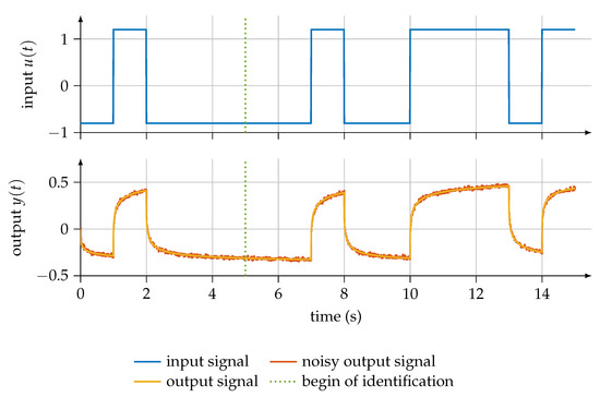
Figure 1. Input and output signals for parameter identification.

To state the model-based auxiliary system, the fractional orders of the boundary terms must first be calculated. Evaluating (25) yields $\gamma =1.35$ and $r=2$. Because $\lceil n\alpha \rceil =1$, the following fractional pseudo state space yields:

$$\left[\begin{array}{c}{\dot{\mathit{x}}}^{\circ }\left(t\right)\\ {}_{t_1}{}^t\mathrm{d}RL_t^{\alpha }{x}^{\square }\left(t\right)\\ {\dot{x}}^{\Delta }\left(t\right)\\ {}_{t_1}{}^t\mathrm{d}RL_t^{\frac{\gamma }{r}}{\mathit{x}}^{\diamond }\left(t\right)\end{array}\right]=\left[\begin{array}{cccccc}0& 0& -\tilde{y}\left(t\right)& 0& 0& 0\\ 0& 0& \tilde{u}\left(t\right)& 0& 0& 0\\ 0& 0& 0& 0& 0& 0\\ 0& 0& 0& 0& 0& 0\\ 0& 0& 0& 0& 0& 1\\ 0& 0& 0& 0& 0& 0\end{array}\right]\left[\begin{array}{c}{\mathit{x}}^{\circ }\left(t\right)\\ x^{\square }\left(t\right)\\ x^{\Delta }\left(t\right)\\ {\mathit{x}}^{\diamond }\left(t\right)\end{array}\right]+\left[\begin{array}{c}0\\ 0\\ 1\\ 1\\ 0\\ 1\end{array}\right]u^{*}\left(t\right)$$

(66)

Depending on the requested parameter, the final pseudo state for $a_0$ is

$$\mathit{x}\left(t_2\right)={\left[\begin{array}{cccccc}1& 0& 0& 0& 0& 0\end{array}\right]}^{\top }$$

(67)

and for $b_0$

$$\mathit{x}\left(t_2\right)={\left[\begin{array}{cccccc}0& 1& 0& 0& 0& 0\end{array}\right]}^{\top }.$$

(68)

The parameter is identified by evaluating (23) and (56) respectively. To calculate the parameter-specific control input, (A32) has to be evaluated. Therefore, the matrix approach of [29] is used.

Because one measurement of the input and output signals can be used to identify all parameters, the parameter-specific control input as well as the trajectories of the parameter estimates for $a_0$ and $b_0$ are illustrated in Figure 2 for the noise-free case and in Figure 3 for the case with a noisy observation of the output signal. The final estimations ${\widehat{a}}_0=2$ and ${\widehat{b}}_0=1$ in the absence of noise and ${\widehat{a}}_0=2.005$ and ${\widehat{b}}_0=0.999$ in the case with a noisy observation of the output signal can be read at the final time of the identification $t_2=10 \mathrm{s}$.

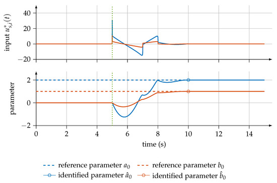
Figure 2. Parameter-specific control input and course of unknown parameter in the noise-free case.

Figure 3. Parameter-specific control input and course of unknown parameter in the case of a noisy observation of the output signal.

The results are compared to the parameter identification using a heuristically adapted modulating function. Because the system is not at rest when the identification is started, the spline-type modulating function has to be used (see [12]). For the approach which is described in this paper, only the starting time and the duration of the identification may be chosen freely. In addition to the start and end times, the use of spline-type modulating functions requires that the number of splines and the order of the modulating function is chosen. It should be noted that the maximum order of the modulating function depends on the number of splines and the minimum order depends on the fractional order of the system (see [12]). All the parameters of the spline-type modulating function have to be fixed a-priori. This is not necessary using the newly proposed method based on implicit modulating functions, from which the modulating function can be determined automatically.

In this example, the method described in [12] is applied using a spline-type modulating function with 20 splines and of order 5 for the comparison. The starting time $t_1=5 \mathrm{s}$ and the identification horizon $5 \mathrm{s}$ are chosen as for the parameter-specific identification method. To derive the independent equations for the linear system (15), the identification horizon has to be shifted. The shifting time is an additional parameter for the identification which is set to $1 \mathrm{s}$ in this example. Using the same input ${\tilde{u}}_o$ and output signal ${\tilde{y}}_o$ illustrated in Figure 1, the parameters are identified to ${\widehat{a}}_0=1.903$ and ${\widehat{b}}_0=0.969$. Regarding the number of shifts, each shift leads to a new independent equation. The linear system (15) consits of $n+m+1$ equations which means that at least $n+m$ shifts are necessary to state the linear system (15). In this example, one shift is sufficient because of $n=1$ and $m=0$ (see (65)). The shifting of the identification horizon makes longer measurements necessary. Considering fractional systems with more parameters, the extension of the measurement duration can be significant. Because of the extension of the measurement duration, more data are considered for parameter identification. Nonetheless, the error of the identified parameters is with 4–5% for the method described in [12] significant greater than the error (approx. 0.3%) made with the parameter-specific approach which is described in this paper.

7. Conclusions

The main contribution of this paper covers the automatic generation of modulating functions by transferring the parameter identification into a control problem, as is provided in Definition (6). For this purpose, a model-based auxiliary system, which connects the fractional-order model, the modulating function as well as the boundary terms resulting from the application of the modulating function method, is defined in this paper. Instead of adjusting a generic modulating function for each parameter individually, it is sufficient to calculate an input signal which steers the model-based auxiliary system from the uninitialized state into the final state (49) corresponding to the parameter to be identified. If the input signal for the steering process is designed as an energy-optimal control, the upper bound of the identification error is minimized in the presence of noisy observations of the input and output signal.

Regarding the practical applicability, the controllability of the model-based auxiliary system is also investigated in this paper and depends on the orders of the fractional-order model and the chosen input signal ${\tilde{u}}_e$ of system (9).

References

- Cesarano, C. Generalized special functions in the description of fractional diffusive equations. Commun. Appl. Ind. Math. 2019, 10, 31–40. [Google Scholar] [CrossRef]
- Bin-Mohsin, B.; Rafique, S.; Cesarano, C.; Javed, M.Z.; Awan, M.U.; Kashuri, A.; Noor, M.A. Some General Fractional Integral Inequalities Involving LR-Bi-Convex Fuzzy Interval-Valued Functions. Fractal Fract. 2022, 6, 565. [Google Scholar] [CrossRef]
- Ospina Agudelo, B.; Zamboni, W.; Monmasson, E. A Comparison of Time-Domain Implementation Methods for Fractional-Order Battery Impedance Models. Energies 2021, 14, 4415. [Google Scholar] [CrossRef]
- Singh, J. Analysis of fractional blood alcohol model with composite fractional derivative. Chaos Solitons Fractals 2020, 140, 110127. [Google Scholar] [CrossRef]
- Kanth, A.S.V.R.; Garg, N. Computational Simulations for Solving a Class of Fractional Models via Caputo-Fabrizio Fractional Derivative. Procedia Comput. Sci. 2017, 125, 476–482. [Google Scholar] [CrossRef]
- Allafi, W.; Zajic, I.; Burnham, K.J. Identification of Fractional Order Models: Application to 1D Solid Diffusion System Model of Lithium Ion Cell. In Progress in Systems Engineering; Selvaraj, H., Zydek, D., Chmaj, G., Eds.; Springer International Publishing: Cham, Switzerland, 2015; pp. 63–68. [Google Scholar]
- Aldoghaither, A.; Liu, D.Y.; Laleg-Kirati, T.M. Modulating Functions Based Algorithm for the Estimation of the Coefficients and Differentiation Order for a Space-Fractional Advection-Dispersion Equation. SIAM J. Sci. Comput. 2015, 37, A2813–A2839. [Google Scholar] [CrossRef]
- Dai, Y.; Wei, Y.; Hu, Y.; Wang, Y. Modulating Function-Based Identification for Fractional Order Systems. Neurocomputing 2016, 173, 1959–1966. [Google Scholar] [CrossRef]
- Eckert, M.; Kupper, M.; Hohmann, S. Functional Fractional Calculus for System Identification of Battery Cells. At–Automatisierungstechnik 2014, 62, 272–281. [Google Scholar] [CrossRef]
- Gao, Z. Modulating Function-Based System Identification for a Fractional-Order System with a Time Delay Involving Measurement Noise Using Least-Squares Method. Int. J. Syst. Sci. 2017, 48, 1460–1471. [Google Scholar] [CrossRef]
- Liu, D.Y.; Laleg-Kirati, T.; Gibaru, O.; Perruquetti, W. Identification of Fractional Order Systems Using Modulating Functions Method. In Proceedings of the American Control Conference (ACC), Washington, DC, USA, 7–19 June 2013; pp. 1679–1684. [Google Scholar]
- Stark, O.; Kupper, M.; Krebs, S.; Hohmann, S. Online Parameter Identification of a Fractional Order Model. In Proceedings of the 57th IEEE Conference on Decision and Control (CDC), Miami, FL, USA, 17–19 December 2018; pp. 2303–2309. [Google Scholar]
- Lu, Y.; Zhang, J.; Tang, Y.G. Parameter Identification of Fractional Order Systems Using a Collocation Method Based on Hybrid Functions. J. Dyn. Syst. Meas. Control 2020, 142, 081007. [Google Scholar] [CrossRef]
- Zhang, B.; Tang, Y.; Zhang, X.; Zhang, C. Parameter Identification of Fractional Order Systems Using a Hybrid of Bernoulli Polynomials and Block Pulse Functions. IEEE Access 2021, 9, 40178–40186. [Google Scholar] [CrossRef]
- Janiczek, T. Generalization of the Modulating Functions Method into the Fractional Differential Equations. Bull. Pol. Acad. Sci. Tech. Sci. 2010, 58, 593–599. [Google Scholar] [CrossRef]
- Schmid, C.; Roppenecker, G. Parameteridentifikation für LTI-Systeme mit Hilfe signalmodellgenerierter Modulationsfunktionen. At–Automatisierungstechnik 2011, 59, 521–528. [Google Scholar] [CrossRef]
- Kilbas, A.A.; Srivastava, H.M.; Trujillo, J.J. Theory and Applications of Fractional Differential Equations, 1st ed.; North-Holland Mathematics Studies; Elsevier: Amsterdam, The Netherlands, 2006; Volume 204. [Google Scholar]
- Lorenzo, C.F.; Hartley, T.T. Initialized Fractional Calculus; Technical Report; NASA Glenn Research Center: Cleveland, OH, USA, 2000. [Google Scholar]
- Eckert, M.; Kölsch, L.; Hohmann, S. Fractional Algebraic Identification of the Distribution of Relaxation Times of Battery Cells. In Proceedings of the 54th IEEE Conference on Decision and Control (CDC), Osaka, Japan, 15–18 December 2015; pp. 2101–2108. [Google Scholar]
- Almeida, R.; Malinowska, A.B.; Torres, D.F.M. A Fractional Calculus of Variations for Multiple Integrals with Application to Vibrating String. J. Math. Phys. 2010, 51, 033503-1–033503-12. [Google Scholar] [CrossRef]
- Lorenzo, C.F.; Hartley, T.T. Initialization, Conceptualization, and Application in the Generalized (Fractional) Calculus. Crit. Rev. Biomed. Eng. 1998, 35, 447–553. [Google Scholar] [CrossRef]
- Podlubny, I. Fractional Differential Equations; Academic Press: Cambridge, UK, 1998. [Google Scholar]
- Samko, S.G.; Kilbas, A.A.; Marichev, O.I. Fractional Integrals and Derivatives: Theory and Applications, 1st ed.; CRC Press: Basel, Switzerland; Philadelphia, PA, USA, 1993. [Google Scholar]
- Isermann, R.; Münchhof, M. Identification of Dynamic Systems: An Introduction with Applications; Springer: Berlin/Heidelberg, Germany, 2011. [Google Scholar]
- Stark, O.; Karg, P.; Hohmann, S. Iterative Method for Online Fractional Order and Parameter Identification. In Proceedings of the 2020 59th IEEE Conference on Decision and Control (CDC), Jeju, Korea, 14–18 December 2020; pp. 5159–5166. [Google Scholar]
- Victor, S.; Malti, R.; Garnier, H.; Oustaloup, A. Parameter and Differentiation Order Estimation in Fractional Models. Automatica 2013, 49, 926–935. [Google Scholar] [CrossRef]
- Shinbrot, M. On the Analysis of Linear and Nonlinear Dynamical Systems from Transient-Response Data; Technical Report; National Advisory Committee for Aeronautics: Moffett Field, CA, USA, 1954. [Google Scholar]
- Eckert, M.; Nagatou-Plum, K.; Rey, F.; Stark, O.; Hohmann, S. Controllability and Energy-Optimal Control of Time-Variant Fractional Systems. In Proceedings of the 57th IEEE Conference on Decision and Control (CDC), Miami, FL, USA, 17–19 December 2018; pp. 4607–4612. [Google Scholar]
- Podlubny, I.; Chechkin, A.V.; Skovranek, T.; Chen, Y.; Jara, B.M.V. Matrix Approach to Discrete Fractional Calculus II: Partial Fractional Differential Equations. J. Comput. Phys. 2009, 228, 3137–3153. [Google Scholar] [CrossRef]
- Bronštejn, I.N.; Semendjaev, K.A.; Musiol, G.; Mühlig, H. Handbook of Mathematics, 6th ed.; Springer: Berlin/Heidelberg, Germany; New York, NY, USA; Dordrecht, The Netherlands; London, UK, 2015. [Google Scholar]
- Kailath, T. Linear Systems; Prentice-Hall: Englewood Cliffs, NJ, USA, 1980. [Google Scholar]
Publisher’s Note: MDPI stays neutral with regard to jurisdictional claims in published maps and institutional affiliations. |
© 2022 by the authors. Licensee MDPI, Basel, Switzerland. This article is an open access article distributed under the terms and conditions of the Creative Commons Attribution (CC BY) license (https://creativecommons.org/licenses/by/4.0/).