
Approximate Closed-Form Solutions for the Maxwell-Bloch Equations via the Optimal Homotopy Asymptotic Method

Abstract
:1. Introduction
2. The Maxwell–Bloch Equations
2.1. Hamilton–Poisson Realization
2.2. Closed-Form Solutions
3. Basic Ideas of the OHAM Technique
- -
- The zeroth-order deformation problem
- -
- The first-order deformation problem
4. Approximate Analytic Solutions via OHAM
4.1. The Zeroth-Order Deformation Problem
4.2. The First-Order Deformation Problem
4.3. The First-Order Analytical Approximate Solution
5. Numerical Results and Discussions
6. Conclusions
Author Contributions
Funding
Institutional Review Board Statement
Informed Consent Statement
Data Availability Statement
Conflicts of Interest
Appendix A

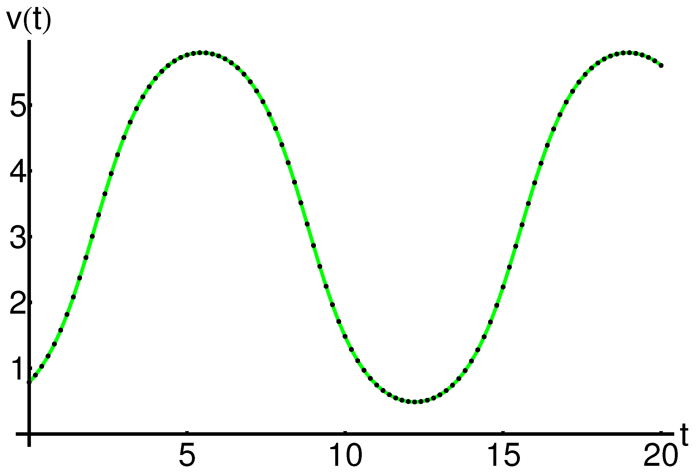
| t | |||
|---|---|---|---|
| 0 | 0.7853981633 | 0.7853981633 | 1.110223 |
| 2 | 3.0048565944 | 3.0048564682 | 1.262252 |
| 4 | 5.4067162901 | 5.4067161112 | 1.789394 |
| 6 | 5.7469951320 | 5.7469952686 | 1.366081 |
| 8 | 4.3979496840 | 4.3979506058 | 9.217917 |
| 10 | 1.4842095296 | 1.4842108567 | 1.327083 |
| 12 | 0.4935555769 | 0.4935555528 | 2.405788 |
| 14 | 1.1089381894 | 1.1089371304 | 1.058989 |
| 16 | 3.8183645538 | 3.8183641247 | 4.291169 |
| 18 | 5.6402614592 | 5.6402619962 | 5.369389 |
| 20 | 5.6036661551 | 5.6036657121 | 4.429515 |
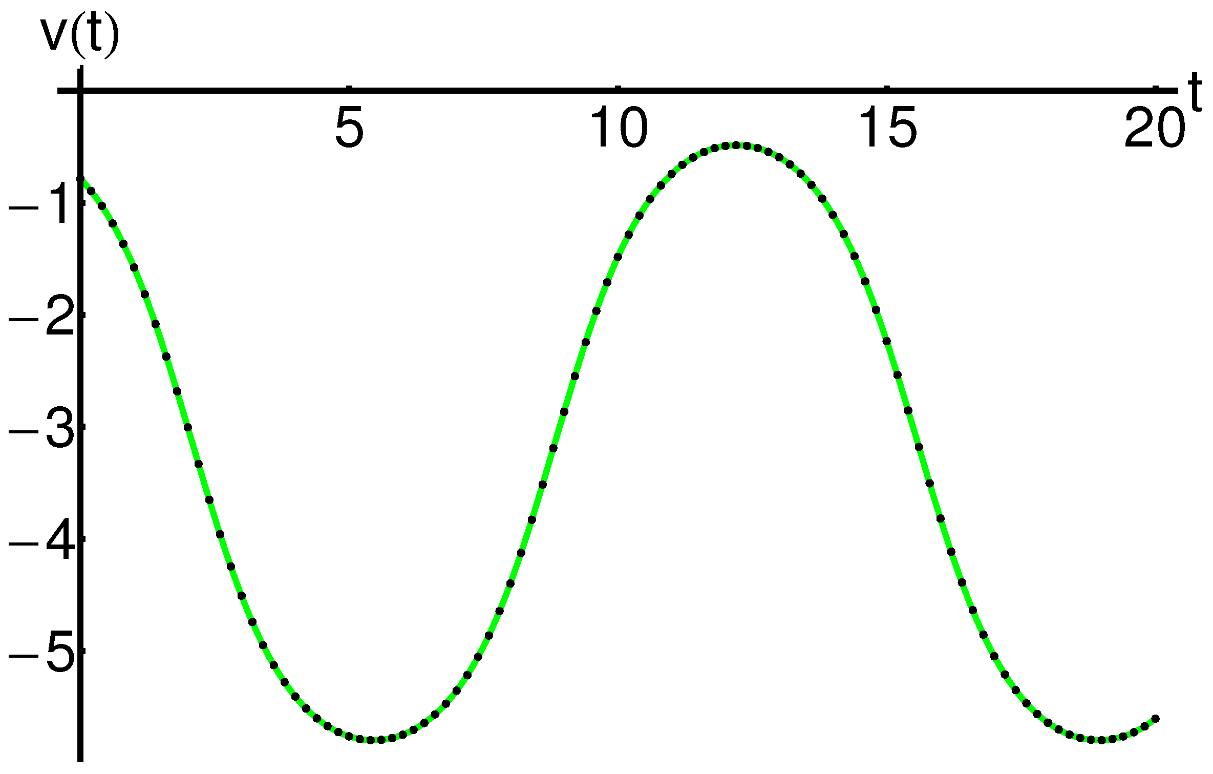
| t | |||
|---|---|---|---|
| 0 | −0.7853981633 | −0.7853981633 | 1.110223 |
| 2 | −3.0048565944 | −3.0048564684 | 1.260096 |
| 4 | −5.4067162901 | −5.4067161110 | 1.790516 |
| 6 | −5.7469951320 | −5.7469952684 | 1.364679 |
| 8 | −4.3979496840 | −4.3979506057 | 9.216750 |
| 10 | −1.4842095296 | −1.4842108566 | 1.326997 |
| 12 | −0.4935555769 | −0.4935555528 | 2.408859 |
| 14 | −1.1089381894 | −1.1089371304 | 1.058966 |
| 16 | −3.8183645538 | −3.8183641248 | 4.290359 |
| 18 | −5.6402614592 | −5.6402619963 | 5.370392 |
| 20 | −5.6036661551 | −5.6036657119 | 4.431479 |
| t | ||||
|---|---|---|---|---|
| 0 | 1.110223 | 8.881784 | 2.220446 | 1.110223 |
| 1/5 | 0.0057507451 | 0.0030455771 | 8.383820 | 1.313631 |
| 2/5 | 0.0227924915 | 0.0070594242 | 8.097412 | 1.229725 |
| 3/5 | 0.0494597939 | 0.0081429073 | 6.156841 | 3.482073 |
| 4/5 | 0.0825167222 | 0.0060042509 | 4.729830 | 6.687728 |
| 1 | 0.1176107773 | 0.0021559238 | 1.174198 | 5.808890 |
| 6/5 | 0.1499196854 | 0.0015691002 | 4.301057 | 3.152192 |
| 7/5 | 0.1749400518 | 0.0039327661 | 6.220876 | 4.754099 |
| 8/5 | 0.1892996460 | 0.0045783745 | 4.222215 | 1.913513 |
| 9/5 | 0.1914052506 | 0.0038272807 | 1.319308 | 2.917863 |
| 2 | 0.1817135046 | 0.0022665042 | 5.933946 | 1.262252 |
References
- Lazureanu, C.; Caplescu, C. Stabilization of the T system by an integrable deformation. In ITM Web of Conferences; Third ICAMNM 2020; EDP Sciences: Les Ulis, France, 2020; Volume 34, p. 03009. [Google Scholar] [CrossRef]
- Braga, D.C.; Dias, F.S.; Mello, L.F. On the stability of the equilibria of the Rikitake system. Phys. Lett. A 2010, 374, 4316–4320. [Google Scholar] [CrossRef]
- Rikitake, T. Oscillations of a system of disk dynamos. Proc. Camb. Philos. Soc. 1958, 54, 89–105. [Google Scholar] [CrossRef]
- Steeb, W.H. Continuous symmetries of the Lorenz model and the Rikitake two-disc dynamo system. J. Phys. A Math. Gen. 1982, 15, 389–390. [Google Scholar] [CrossRef]
- Binzar, T.; Lazureanu, C. On the symmetries of a Rabinovich type system. Sci. Bull. Math. Phys. 2012, 57, 29–36. [Google Scholar]
- Lazureanu, C.; Binzar, T. Symmetries of some classes of dynamical systems. J. Nonlinear Math. Phys. 2015, 22, 265–274. [Google Scholar] [CrossRef] [Green Version]
- Lazureanu, C.; Petrisor, C.; Hedrea, C. On a deformed version of the two-disk dynamo system. Appl. Math. 2021, 66, 345–372. [Google Scholar] [CrossRef]
- Lazureanu, C.; Petrisor, C. Stability and energy-Casimir Mapping for integrable deformations of the Kermack-McKendrick system. Adv. Math. Phys. 2018, 2018, 5398768. [Google Scholar] [CrossRef]
- Lazureanu, C. Integrable deformations of three-dimensional chaotic systems. Int. J. Bifurcat. Chaos 2018, 28, 1850066. [Google Scholar] [CrossRef]
- Lazureanu, C. Hamilton-Poisson realizations of the integrable deformations of the Rikitake system. Adv. Math. Phys. 2017, 2017, 4596951. [Google Scholar] [CrossRef] [Green Version]
- Lazureanu, C. The real-valued Maxwell-Bloch equations with controls: From a Hamilton-Poisson system to a chaotic one. Int. J. Bifurcat. Chaos 2017, 27, 1750143. [Google Scholar] [CrossRef]
- Lazureanu, C. On a Hamilton-Poisson approach of the Maxwell-Bloch equations with a control. Math. Phys. Anal. Geom. 2017, 20, 20. [Google Scholar] [CrossRef]
- Lazureanu, C.; Binzar, T. Symmetries and properties of the energy-Casimir mapping in the ball-plate problem. Adv. Math. 2017, 2017, 5164602. [Google Scholar] [CrossRef] [Green Version]
- Lazureanu, C.; Binzar, T. On some properties and symmetries of the 5-dimensional Lorenz system. Math. Probl. Eng. 2015, 2015, 438694. [Google Scholar] [CrossRef]
- Lazureanu, C.; Binzar, T. Some symmetries of a Rossler type system. Sci. Bull. Math. Phys. 2013, 58, 1–6. [Google Scholar]
- Binzar, T.; Lazureanu, C. A Rikitake type system with one control. Discrete Contin. Dyn. B 2013, 18, 1755–1776. [Google Scholar] [CrossRef]
- Lazureanu, C.; Binzar, T. Symplectic realizations and symmetries of a Lotka-Volterra type system. Regul. Chaotic Dyn. 2013, 18, 203–213. [Google Scholar] [CrossRef] [Green Version]
- Lazureanu, C.; Binzar, T. A Rikitake type system with quadratic control. Int. J. Bifur. Chaos 2012, 22, 1250274. [Google Scholar] [CrossRef]
- Lazureanu, C.; Binzar, T. On the symmetries of a Rikitake type system. Comptes Rendus Math. Acad. Sci. Paris 2012, 350, 529–533. [Google Scholar] [CrossRef] [Green Version]
- Lazureanu, C. On the Hamilton-Poisson realizations of the integrable deformations of the Maxwell-Bloch equations. Comptes Rendus Acad. Sci. Paris Ser. I 2017, 355, 596–600. [Google Scholar] [CrossRef]
- Candido Murilo, R.; Llibre, J.; Valls, C. New symmetric periodic solutions for the Maxwell-Bloch differential system. Math. Phys. Anal. Geom. 2019, 22, 16. [Google Scholar] [CrossRef]
- David, D.; Holm, D. Multiple Lie–Poisson structures, reduction and geometric phases for the Maxwell–Bloch traveling wave equations. J. Nonlinear Sci. 1992, 2, 241–262. [Google Scholar] [CrossRef]
- Puta, M. On the Maxwell–Bloch equations with one control. Comptes Rendus Acad. Sci. Paris Serie I 1994, 318, 679–683. [Google Scholar]
- Puta, M. Three dimensional real valued Maxwell–Bloch equations with controls. Rep. Math. Phys. 1996, 3, 337–348. [Google Scholar] [CrossRef]
- Arecchi, F.T. Chaos and generalized multistability in quantum optics. Phys. Scr. 1985, 9, 85–92. [Google Scholar] [CrossRef]
- Casu, I.; Lazureanu, C. Stability and integrability aspects for the Maxwell-Bloch equations with the rotating wave approximation. Regul. Chaotic Dyn. 2017, 22, 109–121. [Google Scholar] [CrossRef]
- Zuo, D.W. Modulation instability and breathers synchronization of the nonlinear Schrodinger Maxwell–Bloch equation. Appl. Math. Lett. 2018, 79, 182–186. [Google Scholar] [CrossRef]
- Wang, L.; Wang, Z.Q.; Sun, W.R.; Shi, Y.Y.; Li, M.; Xu, M. Dynamics of Peregrine combs and Peregrine walls in an inhomogeneous Hirota and Maxwell–Bloch system. Commun. Nonlinear Sci. Numer. Simul. 2017, 47, 190–199. [Google Scholar] [CrossRef]
- Wei, J.; Wang, X.; Geng, X. Periodic and rational solutions of the reduced Maxwell–Bloch equations. Commun. Nonlinear Sci. Numer. Simul. 2018, 59, 1–14. [Google Scholar] [CrossRef] [Green Version]
- Binzar, T.; Lazureanu, C. On some dynamical and geometrical properties of the Maxwell–Bloch equations with a quadratic control. J. Geom. Phys. 2013, 70, 1–8. [Google Scholar] [CrossRef]
- Puta, M. Integrability and geometric prequantization of the Maxwell-Bloch equations. Bull. Sci. Math. 1998, 122, 243–250. [Google Scholar] [CrossRef] [Green Version]
- El-Rashidy, K.; Seadawy, A.R.; Althobaiti, S.; Makhlou, M.M. Multiwave, Kinky breathers and multi-peak soliton solutions for the nonlinear Hirota dynamical system. Results Phys. 2020, 19, 103678. [Google Scholar] [CrossRef]
- Amer, T.S.; Bek, M.A.; Hassan, S.S.; Elbendary, S. The stability analysis for the motion of a nonlinear damped vibrating dynamical system with three-degrees-of-freedom. Results Phys. 2021, 28, 104561. [Google Scholar] [CrossRef]
- Marinca, V.; Herisanu, N. Nonlinear dynamic analysis of an electrical machine rotor-bearing system by the optimal homotopy perturbation method. Comput. Math. Appl. 2011, 61, 2019–2024. [Google Scholar] [CrossRef] [Green Version]
- Marinca, V.; Ene, R.D.; Marinca, B. Optimal Homotopy Perturbation Method for nonlinear problems with applications. Appl. Comp. Math. 2022, 21, 123–136. [Google Scholar]
- Bota, C.; Caruntu, B.; Tucu, D.; Lapadat, M.; Pasca, M.S. A Least Squares Differential Quadrature Method for a Class of Nonlinear Partial Differential Equations of Fractional Order. Mathematics 2020, 8, 1336. [Google Scholar] [CrossRef]
- Caruntu, B.; Bota, C.; Lapadat, M.; Pasca, M.S. Polynomial Least Squares Method for Fractional Lane-Emden Equations. Symmetry 2019, 11, 479. [Google Scholar] [CrossRef] [Green Version]
- Marinca, V.; Draganescu, G.E. Construction of approximate periodic solutions to a modified van der Pol oscillator. Nonlinear Anal. Real World Appl. 2010, 11, 4355–4362. [Google Scholar] [CrossRef]
- Herisanu, N.; Marinca, V. Accurate analytical solutions to oscillators with discontinuities and fractional-power restoring force by means of the optimal homotopy asymptotic method. Comput. Math. Appl. 2010, 60, 1607–1615. [Google Scholar] [CrossRef] [Green Version]
- Safdar, H.; Abdullah, S.; Sana, A.; Asad, U. An approximate analytical solution of the Allen-Cahn equation using homotopy perturbation method and homotopy analysis method. Heliyon 2019, 5, e03060. [Google Scholar]
- Wang, X.; Xu, Q.; Atluri, S.N. Combination of the variational iteration method and numerical algorithms for nonlinear problems. Appl. Math. Model. 2020, 79, 243–259. [Google Scholar] [CrossRef]
- Turkyilmazoglu, M. An optimal variational iteration method. Appl. Math. Lett. 2011, 24, 762–765. [Google Scholar] [CrossRef] [Green Version]
- Han, C.; Wang, Y.-L. Numerical Solutions of Variable-Coefficient Fractional-in-Space KdV Equation with the Caputo Fractional Derivative. Fractal Fract. 2022, 6, 207. [Google Scholar] [CrossRef]
- Li, Z.; Chen, Q.; Wang, Y.; Li, X. Solving Two-Sided Fractional Super-Diffusive Partial Differential Equations with Variable Coefficients in a Class of New Reproducing Kernel Spaces. Fractal Fract. 2022, 6, 492. [Google Scholar] [CrossRef]
- Marinca, V.; Herisanu, N. The Optimal Homotopy Asymptotic Method—Engineering Applications; Springer: Berlin/Heidelberg, Germany, 2015. [Google Scholar]
- Paşca, M.S.; Bundău, O.; Juratoni, A.; Căruntu, B. The Least Squares Homotopy Perturbation Method for Systems of Differential Equations with Application to a Blood Flow Model. Mathematics 2022, 10, 546. [Google Scholar] [CrossRef]

Publisher’s Note: MDPI stays neutral with regard to jurisdictional claims in published maps and institutional affiliations. |
© 2022 by the authors. Licensee MDPI, Basel, Switzerland. This article is an open access article distributed under the terms and conditions of the Creative Commons Attribution (CC BY) license (https://creativecommons.org/licenses/by/4.0/).
Share and Cite
Ene, R.-D.; Pop, N.; Lapadat, M.; Dungan, L. Approximate Closed-Form Solutions for the Maxwell-Bloch Equations via the Optimal Homotopy Asymptotic Method. Mathematics 2022, 10, 4118. https://doi.org/10.3390/math10214118
Ene R-D, Pop N, Lapadat M, Dungan L. Approximate Closed-Form Solutions for the Maxwell-Bloch Equations via the Optimal Homotopy Asymptotic Method. Mathematics. 2022; 10(21):4118. https://doi.org/10.3390/math10214118
Chicago/Turabian StyleEne, Remus-Daniel, Nicolina Pop, Marioara Lapadat, and Luisa Dungan. 2022. "Approximate Closed-Form Solutions for the Maxwell-Bloch Equations via the Optimal Homotopy Asymptotic Method" Mathematics 10, no. 21: 4118. https://doi.org/10.3390/math10214118