On the Non-Local Boundary Value Problem from the Probabilistic Viewpoint

Abstract

We provide a short introduction of new and well-known facts relating non-local operators and irregular domains. Cauchy problems and boundary value problems are considered in case non-local operators are involved. Such problems lead to anomalous behavior on the bulk and on the surface of a given domain, respectively. Such a behavior should be considered (in a macroscopic viewpoint) in order to describe regular motion on irregular domains (in the microscopic viewpoint).

1. Introduction

We present a collection of results about the connection between non-local operators and irregular domains. We are concerned with the interplay between macroscopic and microscopic analysis of Feller motions on bounded and unbounded domains. Our discussion relies on the fact that anomalous motions on regular domains can be considered in order to describe motions on irregular domains. Here, by irregular domains we mean domains with irregular boundaries or interfaces, for example, of the fractal type.

Fractional Cauchy problems have been considered as models for motions on non-homogeneous domains, for instance, fractals. In the same spirit, we consider anomalous motions for non-local boundary value problems, that is, the motions exhibit anomalous behavior only near the boundary. Non-local boundary conditions therefore introduce models for motions on irregular domains, for example, domains with trap boundaries (trap domains, in the sequel).

The presentation will run as follows. First, we recall some facts about non-local operators and the associated processes. Sometimes, non-local operators are also referred to as generalized fractional operators. However, there is no fractional order to be considered. We move to the next sections by discussing the non-local initial value problems and then the non-local boundary value problems. For the latter, we underline some connection with the case of random Koch domains and, in particular, with the boundary behaviors introduced by the non-local boundary conditions.

2. Markov Processes, Time Changes, Non-Local Operators

2.1. Markov Processes

Let $X={\left\{X_t\right\}}_{t\ge 0}$ with $X_0=x\in \Omega$ be the Markov process on $\Omega$ with generator $(G,D(G\left)\right)$, where $(G,D(G\left)\right)$ is the generator of the semigroup $Q_t$; then, we have the following probabilistic representation:

$$\begin{array}{c}\hfill Q_{t}f\left(x\right)={\mathbf{E}}_x\left[f\left(X_t\right)\right].\end{array}$$

We recall that for the Markovian semigroup $Q_t$, the generator is defined by:

$$\begin{array}{c}\hfill Gf\left(x\right)=\underset{t\downarrow 0}{lim}\frac{Q_{t}f\left(x\right)-f\left(x\right)}{t},f\in D\left(G\right)\end{array}$$

(1)

for f in some set of real-valued functions and for which the limit exists in some sense. Then, we say that f belongs to the domain of the generator $D\left(G\right)$. In case X is a Feller process for instance, the domain $D\left(G\right)$ consists of continuous functions vanishing at infinity for which (1) exists as a uniform limit. Examples of Feller processes are given by the Brownian motion (with $Gf=f^{″}$), the Poisson process (with $Gf=\lambda (F-1)f$ where $Ff\left(x\right)=f(x+1)$ is the forward operator) and, in general, Lévy processes (for which we will consider $G=-\Psi (-\Delta )$ to be better defined further on). For the Brownian motion, the forward and backward Kolmogorov’s equation have the same reading in terms of heat equations. A Poisson process (started at zero, for instance) is driven by $\lambda (1-B)f$, where $Bf\left(x\right)=f(x-1)$ is the backward operator. We skip here a discussion on Lévy processes.

We say that X is a Feller process if X is a strong Markov process that is right-continuous with no discontinuity other than jumps. If X is a continuous strong Markov process, we say that X is a Feller diffusion (or simply, diffusion).

For the process X started at x with density $p(t,x,y)$, it holds that

$$\begin{array}{c}\hfill {\mathbf{P}}_x(X_t\in D)={\int }_{D}p(t,x,y)dy,D\subseteq \Omega \end{array}$$

and

$$\begin{array}{c}\hfill {\mathbf{E}}_x\left[f\left(X_t\right)\right]={\int }_{\Omega }f\left(y\right)p(t,x,y)dy,t>0,x\in \Omega \end{array}$$

where ${\mathbf{E}}_x$ is the expectation with respect to ${\mathbf{P}}_x$. The function $u(t,x)=Q_{t}f\left(x\right)$ solves the Cauchy problem:

$$\begin{array}{c}\hfill \frac{\partial u}{\partial t}=Gu,u_0=f\in D\left(G\right).\end{array}$$

2.2. Subordinators and Inverses

The Bernstein function

$$\Phi \left(\lambda \right)={\int }_0^{\infty }\left(1-e^{-\lambda z}\right)\varphi \left(dz\right),\lambda \ge 0$$

(2)

where $\varphi$ on $(0,\infty )$ with ${\int }_0^{\infty }(1\wedge z)\varphi \left(dz\right)<\infty$, is now a Lévy measure and can be associated with a Lévy process. Thus, the symbol $\Phi$ is the Laplace exponent of a subordinator $H_t$ with $H_0=0$, that is,

$${\mathbf{E}}_0[exp(-\lambda H_t)]=exp(-t\Phi \left(\lambda \right)).$$

We also recall that

$$\begin{array}{c}\hfill \frac{\Phi \left(\lambda \right)}{\lambda }={\int }_0^{\infty }{e}^{-\lambda z}\overline{\varphi }\left(z\right)dz,\overline{\varphi }\left(z\right)=\varphi \left((z,\infty )\right)={\int }_z^{\infty }\varphi \left(d\mathfrak{z}\right)\end{array}$$

(3)

and $\overline{\varphi }$ is the so-called tail of the Lévy measure.

Let us introduce the inverse process

$$L_t:=inf\{s\ge 0:H_s\ge t\}=inf\{s\ge 0:H_s\notin (0,t)\}$$

with $L_0=0$. We do not consider (except in some well-mentioned case) step-processes with $\varphi \left(\right(0,\infty \left)\right)<\infty$, and therefore, we focus only on strictly increasing subordinators with infinite measures. Thus, the inverse process L turns out to be a continuous process. Both random times H and L are not decreasing. By definition, we also can write:

$$\begin{array}{c}\hfill {\mathbf{P}}_0(H_t<s)={\mathbf{P}}_0(L_s>t),s,t>0.\end{array}$$

(4)

It is worth noting that H can be regarded as a hitting time for a Markov process, whereas L can be regarded as a local time for a Markov process [1]. We denote by h and l the following densities:

$$\begin{array}{c}\hfill {\mathbf{P}}_0(H_t\in dx)=h(t,x)dx,{\mathbf{P}}_0(L_t\in dx)=l(t,x)dx.\end{array}$$

As usual, we denote by ${\mathbf{P}}_0$ the probability of a process started at $x=0$.

Remark 1.

For $\Phi \left(\lambda \right)={\lambda }^{\alpha }$ (that is, for stable subordinators), the following relation between densities holds:

$$\begin{array}{c}\hfill \frac{h(v,z)}{l(z,v)}=\alpha \frac{v}{z},z,v>0.\end{array}$$

This result has been stated in the famous book [1] without proof; thus, we refer to [2].

From (4), straightforward calculation gives:

$$\begin{array}{c}\hfill {\int }_0^{\infty }{e}^{-\lambda t}l(t,x)dt=\frac{\Phi \left(\lambda \right)}{\lambda }{e}^{-x\Phi \left(\lambda \right)},\lambda >0.\end{array}$$

(5)

It suffices to consider that

$$l(t,x)=-\frac{d}{dx}{\mathbf{P}}_0(L_t>x)=-\frac{d}{dx}{\mathbf{P}}_0(t>H_x)$$

in (5). We recall that [3], for a good function f, for $\lambda >{\Phi }^{-1}\left(w\right)$:

$${\mathbf{E}}_0\left[{\int }_0^{\infty }{e}^{-\lambda t}f\left(L_t\right)dt\right]=\frac{\Phi \left(\lambda \right)}{\lambda }{\mathbf{E}}_0\left[{\int }_0^{\infty }{e}^{-\lambda H_t}f\left(t\right)dt\right].$$

(6)

Denote by $\tilde{l}(\lambda ,x)$ the Laplace transform (5). Assume that $\forall x>0$, for $n\ge 1$:

$$\begin{array}{c}\hfill \underset{\lambda \to 0^{+}}{lim}{\lambda }^n\tilde{l}(\lambda ,x)=0\mathrm{and}\underset{\lambda \to \infty }{lim}{\lambda }^n\tilde{l}(\lambda ,x)=0.\end{array}$$

(7)

Then, we conclude that $\forall x>0$, for $n\ge 1,$${\lambda }^n\tilde{l}(\lambda ,x)\in C_0[0,\infty )$ and in particular:

$$\begin{array}{c}\hfill \exists M>0:\forall x>0,|{\lambda }^n\tilde{l}(\lambda ,x)|\le M.\end{array}$$

Thus, under (7):

$$\begin{array}{c}\hfill \forall x>0l(·,x)\in C^{\infty }(0,\infty ).\end{array}$$

A further check shows that ($n=0$ and Formula (5)):

$$\begin{array}{c}\hfill \forall x>0l(·,x)\in L_1(0,\infty )\mathrm{iff}\underset{\lambda \downarrow 0}{lim}\frac{\Phi \left(\lambda \right)}{\lambda }<\infty .\end{array}$$

Concerning $\tilde{h}(t,\xi )=e^{-t\Phi \left(\xi \right)}$, assume that $\forall t>0$, for $n\ge 1$, ${\xi }^n\tilde{h}(t,\xi )\in C_0[0,\infty )$, and therefore, ${\xi }^n\tilde{h}(t,\xi )$ is bounded as well. Then, we have that

$$\begin{array}{c}\hfill \forall t>0h(t,·)\in C^{\infty }(0,\infty ).\end{array}$$

Here, we obviously have that

$$\begin{array}{c}\hfill \forall t>0h(t,·)\in L_1(0,\infty ).\end{array}$$

Remark 2.

We notice that the Laplace transform $\widehat{u}\left(\lambda \right)$ with $\lambda >\omega$ exists for u in the set of piecewise continuous functions of exponential order w. That is, given $M>0$, $\exists T$ such that $\left|u\left(t\right)\right|\le M{e}^{t\omega }$ for $t>T$. This fact will be also discussed further on.

Proposition 1.

We have that $l(z,0)=\overline{\varphi }\left(z\right)$, $z>0$.

Proof. 

Just considering (5). □

Proposition 2.

Let us write:

$$\begin{array}{c}\hfill \kappa \left(z\right)={\int }_0^{\infty }h(t,z)dt,\mathit{and}\ell \left(z\right)=l(z,0),z>0.\end{array}$$

Then, κ and ℓ are associated Sonine kernels. Moreover,

$$\begin{array}{c}\hfill {\int }_{\mathbb{R}}\kappa \left(z\right)\ell (1-z)dz={\int }_0^1\kappa \left(z\right)\ell (1-z)dz=1.\end{array}$$

(8)

Proof. 

It is enough to consider the Laplace transforms of $\kappa$ and ℓ. □

We notice that, for a stable subordinator, for which $\Phi \left(z\right)=z^{\alpha }$:

$$\begin{array}{c}\hfill {\mathbf{E}}_0\left[{\int }_0^{\infty }{e}^{-\lambda H_t}dt\right]=\frac{1}{{\lambda }^{\alpha }}={\int }_0^{\infty }{e}^{-\lambda x}\frac{x^{\alpha -1}}{\Gamma \left(\alpha \right)}dx\end{array}$$

from which we obtain the potential density of $H_t$, that is,

$$\begin{array}{c}\hfill {\int }_0^{\infty }h(t,x)dt=\frac{x^{\alpha -1}}{\Gamma \left(\alpha \right)}=:\kappa \left(x\right),x>0.\end{array}$$

The inverse of ${\lambda }^{\alpha -1}$ gives:

$$\begin{array}{c}\hfill l(t,0)=\frac{t^{-\alpha }}{\Gamma (1-\alpha )}=:\ell \left(t\right),t>0.\end{array}$$

Thus, Formula (8) is verified. The convolutions $\kappa \ast u$ and $\ell \ast u$ can be used in order to define the fractional integral and the fractional derivative of a given function u, respectively. Indeed,

$$\begin{array}{c}\hfill {\mathcal{D}}_x^{\alpha }u\left(x\right):=\frac{d}{dx}{\mathcal{I}}_x^{1-\alpha }u\left(x\right)=\frac{1}{\Gamma (1-\alpha )}\frac{d}{dx}{\int }_0^{x}u\left(y\right){(x-y)}^{-\alpha }dy\end{array}$$

is the well-known Riemann–Liouville derivative written in terms of the associated fractional integral. Notice that

$$\begin{array}{c}\hfill {\mathcal{D}}_x^{\alpha }u\left(x\right)=\frac{d}{dx}(u\ast \ell )\left(x\right),{\mathcal{I}}_x^{\alpha }u\left(x\right)=(u\ast \kappa )\left(x\right).\end{array}$$

We also recall the Caputo–Dzherbashian derivative:

$$\begin{array}{c}\hfill D_x^{\alpha }u\left(x\right):=\frac{1}{\Gamma (1-\alpha )}{\int }_0^x{u}^{\prime }\left(s\right){(x-s)}^{-\alpha }ds={\mathcal{D}}_x^{\alpha }\left(u\left(x\right)-u\left(0\right)\right)\end{array}$$

where $u^{\prime }=du/ds$. The Caputo–Dzherbashian derivative (also termed the Caputo derivative) was introduced by Caputo in [4,5,6] and previously by Dzherbashian in [7,8]. The Riemann–Liouville derivatives have a long history.

The previous operators are obtained by convolution and represent well-known objects in fractional calculus where $\alpha$ has a clear meaning in terms of fractional order. Some criticisms have been also reported in the literature about the definition of derivative and integral for some operators (see, for example, [9]). In the following, we consider non-local operators for which we do not have a direct link with a fractional order but with a symbol $\Phi$ and, therefore, with a convolution kernel (singular or not, see the last section). We basically move from the following “types” of operators:

(i)

Marchaud (type) operators:

$$\begin{array}{c}\hfill {\mathbf{D}}_{x-}^{\Phi }u\left(x\right)={\int }_0^{\infty }\left(u\left(x\right)-u(x-y)\right)\varphi \left(dy\right)\end{array}$$

and

$$\begin{array}{c}\hfill {\mathbf{D}}_{x+}^{\Phi }u\left(x\right)={\int }_0^{\infty }\left(u\left(x\right)-u(x+y)\right)\varphi \left(dy\right);\end{array}$$

(ii)

Riemann–Liouville (type) operators:

$$\begin{array}{c}\hfill {\mathcal{D}}_{x-}^{\Phi }u\left(x\right)=\frac{d}{dx}{\int }_{-\infty }^{x}u(x-y)\overline{\varphi }\left(y\right)dy\end{array}$$

and

$$\begin{array}{c}\hfill {\mathcal{D}}_{x+}^{\Phi }u\left(x\right)=\frac{d}{dx}{\int }_x^{\infty }u(x-y)\overline{\varphi }\left(y\right)dy;\end{array}$$

(iii)

Caputo–Dzherbashian (type) operators

$$\begin{array}{c}\hfill {\mathfrak{D}}_t^{\Phi }u\left(t\right)={\int }_0^t{u}^{\prime }(t-s)\overline{\varphi }\left(y\right)dy\end{array}$$

where $u^{\prime }=du/dt$ is the derivative of $u\left(t\right)$.

These operators coincide in a certain class of functions. A key fact is played by the extension of zero for the negative part of the real line. That is, for those functions u for which $u\left(x\right)=0$ for $x\le 0$, a quick check shows that, under the right assumptions for the existence of Laplace transforms in each definition, the Laplace symbols coincide.

2.3. Non-Local (Space) Operators

Let $(G,D(G\left)\right)$ be the generator of the semigroup $Q_t$. We consider the representation:

$$\begin{array}{c}\hfill -\Phi (-G)f\left(x\right)={\int }_0^{\infty }\left(Q_{t}f\left(x\right)-f\left(x\right)\right)\varphi \left(dt\right)\end{array}$$

(9)

given by Phillips, where $\Phi$ has been introduced in (2). This nice representation has been considered in [10] and previously for $G=\Delta$ in [11]. Indeed, in case of subordinate Brownian semigroups obtained via stable measure, we also refer to Bochner’s subordination. For a general Markov process with generator G we refer to Phillips. Let $\Psi$ be the Fourier multiplier of G. Then, the Fourier symbol of the semigroup $Q_t=e^{tG}$ is written as $\widehat{Q_t}=e^{-t\Psi }$. For a well-defined function f, from (2) we have that

$$\begin{array}{cc}\hfill {\int }_{\mathbb{R}}{e}^{i\xi x}\left(-\Phi (-G)f\left(x\right)\right)dx=& \left({\int }_0^{\infty }\left(e^{-t\Psi \left(\xi \right)}-1\right)\varphi \left(dt\right)\right)\widehat{f}\left(\xi \right)\hfill \\ \hfill =& -\Phi \circ \Psi \left(\xi \right)\widehat{f}\left(\xi \right).\hfill \end{array}$$

Thus, $\Phi \circ \Psi$ is the Fourier multiplier of $A=-\Phi (-G)$.

Remark 3.

The subordinator H, with symbol Φ, has a density h satisfying

$${\partial }_{t}h=-\Phi \left({\partial }_x\right)h.$$

See the Phillips’ representation with the translation semigroup

$$e^{-t{\partial }_x}v\left(x\right)=v(x-t).$$

Remark 4.

We observe that

$$\begin{array}{c}\hfill D_x^{\alpha }u\left(x\right)=\Phi \left({\partial }_x\right)u\left(x\right)-\frac{x^{-\alpha }}{\Gamma (1-\alpha )}u\left(0\right)\end{array}$$

where ${\partial }_x=\partial /\partial x$ is the first partial derivative, the generator of the translation semigroup. Thus, $\Phi \left({\partial }_x\right)u\left(x\right)$ gives a Riemann–Liouville operator.

Remark 5.

(Dirichlet boundary condition) In a general setting, for compact domains, we have the compact representation:

$$\begin{array}{c}\hfill \Phi (-{\Delta }_{\Omega })v\left(x\right)=\sum _k\Phi \left({\mu }_k\right)(v,e_k)e_k\left(x\right),x\in \Omega \end{array}$$

(10)

with $v\left(x\right)=0$ if $x\in \partial \Omega$. A sketch of proof can be given by considering that

$$\begin{array}{c}\hfill Q_t{e}_k\left(x\right)=e^{-t{\mu }_k}{e}_k\left(x\right).\end{array}$$

From the Phillips’ representation and the fact that

$$\begin{array}{c}\hfill v\left(x\right)=\sum _k(v,e_k)e_k\left(x\right)\end{array}$$

We obtain (10). Then, the equation is satisfied term-by-term, the convergence is easily verified by considering the suitable space $H^s$ of functions $v\in L^2$ such that ${\sum }_k{\left({\mu }_k\right)}^{2s}(v,e_k)<\infty$. Observe that $\Phi \left({\mu }_k\right)$ is written as in (2); thus, the spectral representation (10) coincides with (9).

Remark 6.

We note that if H is the stable subordinator with symbol $\Phi \left(\xi \right)={\xi }^{\alpha }$ and $Q_t$ is the semigroup of a Brownian motion on ${\mathbb{R}}^d$ with $\Psi \left(\xi \right)={\left|\xi \right|}^2$, then ${\left|\xi \right|}^{2\alpha }$ is the symbol $\Psi \circ \Phi$ of the fractional Laplacian:

$$\begin{array}{c}\hfill -\Phi (-G)=-{(-\Delta )}^{\alpha },\alpha \in (0,1)\end{array}$$

(11)

where ${(-\Delta )}^{\alpha }u$ is defined as Cauchy principal value. The Phillips’ representation (11) holds only on ${\mathbb{R}}^d$, $d\ge 1$. We underline that the Phillips’ representation on $\Omega \subset {\mathbb{R}}^d$ coincides with the spectral definition $-{(-{\Delta }_{\Omega })}^{\alpha }$, where $({\Delta }_{\Omega },D\left({\Delta }_{\Omega }\right))$ is the generator of a Brownian motion on Ω. Thus, we obtain $-\Phi (-{\Delta }_{\Omega })$ as in (10) in case ${\Delta }_{\Omega }$ is the Dirichlet Laplacian.

2.4. Non-Local (Time) Operators

Let $M>0$ and $w\ge 0$. Let ${\mathcal{M}}_w$ be the set of (piecewise) continuous functions on $[0,\infty )$ of exponential order w such that $\left|u\left(t\right)\right|\le M{e}^{wt}$. Denote by $\tilde{u}$ the Laplace transform of u. Then, we define the operator ${\mathfrak{D}}_t^{\Phi }:{\mathcal{M}}_w\mapsto {\mathcal{M}}_w$ such that

$$\begin{array}{c}\hfill {\int }_0^{\infty }{e}^{-\lambda t}{\mathfrak{D}}_t^{\Phi }u\left(t\right)dt=\Phi \left(\lambda \right)\tilde{u}\left(\lambda \right)-\frac{\Phi \left(\lambda \right)}{\lambda }u\left(0\right),\lambda >w\end{array}$$

(12)

where $\Phi$ is given in (2). Since u is exponentially bounded, the integral $\tilde{u}$ is absolutely convergent for $\lambda >w$. By Lerch’s theorem the inverse Laplace transforms u and ${\mathfrak{D}}_t^{\Phi }u$ are uniquely defined. We note that

$$\begin{array}{cc}\hfill \Phi \left(\lambda \right)\tilde{u}\left(\lambda \right)-\frac{\Phi \left(\lambda \right)}{\lambda }u\left(0\right)=& \left(\lambda \tilde{u}\left(\lambda \right)-u\left(0\right)\right)\frac{\Phi \left(\lambda \right)}{\lambda }\hfill \end{array}$$

(13)

and thus, ${\mathfrak{D}}_t^{\Phi }$ can be written as a convolution involving the ordinary derivative and the inverse transform of (3) iff $u\in {\mathcal{M}}_w\cap C([0,\infty ),{\mathbb{R}}_{+})$ and $u^{\prime }\in {\mathcal{M}}_w$. By Young’s convolution inequality we obtain

$$\begin{array}{c}\hfill {\int }_0^{\infty }{\left|{\mathfrak{D}}_t^{\Phi }u\right|}^{p}dt\le \left({\int }_0^{\infty }{\left|u^{\prime }\right|}^{p}dt\right){\left(\underset{\lambda \downarrow 0}{lim}\frac{\Phi \left(\lambda \right)}{\lambda }\right)}^p,p\in [1,\infty )\end{array}$$

(14)

where ${lim}_{\lambda \downarrow 0}\Phi \left(\lambda \right)/\lambda$ is finite only in some cases. Indeed, suppose that $f\in L_p\left(\mathbb{R}\right)$, $g\in L_q\left(\mathbb{R}\right)$ and $1/p+1/q=1/r+1$ with $1\le p,q,r\le \infty$. Then,

$$\begin{array}{c}\hfill {\parallel f\ast g\parallel }_r\le {\parallel f\parallel }_p{\parallel g\parallel }_q.\end{array}$$

Now set $f=u^{\prime }$ and $g=\overline{\varphi }$. Take the limit for $\lambda \to 0^{+}$ of the Laplace transform $\tilde{g}\left(\lambda \right)$ in order to obtain ${\parallel g\parallel }_1$.

We notice that when $\Phi \left(\lambda \right)=\lambda$ (that is, when we deal with the ordinary derivative), we have that $H_t=t$ and $L_t=t$ a.s., and in (14), the equality holds. We observe that ${\mathfrak{D}}_t^{\Phi }u$ is well-defined for u such that $u,u^{\prime }\in {\mathcal{M}}_w$. For $w=0$, $u\in C_b[0,\infty )$ is a Lipschitz function on $[0,\infty )$. Indeed, we are considering u with (piecewise) continuous and bounded derivative. Formula (14) gives the relevant information stated in the following propositions.

Proposition 3.

Let Φ be such that

$$\begin{array}{c}\hfill \underset{\lambda \downarrow 0}{lim}\frac{\Phi \left(\lambda \right)}{\lambda }={\Phi }_0<\infty .\end{array}$$

If $u\in AC[0,\infty )$, then ${\mathfrak{D}}_t^{\Phi }u\in L_1[0,\infty )$.

Proof. 

The statement follows from (14) for $p=1$. □

Proposition 4.

Let us consider the parabolic problem ${\mathfrak{D}}_t^{\Phi }u=Au$ for some generator $(A,D(A\left)\right)$ and a given Φ. Then, the existence of the corresponding elliptic problem $-A\overline{u}={\Phi }_{0}f$ is given according to (14).

Proof. 

Let us consider $\overline{u}\left(x\right)={\int }_0^{\infty }u(t,x)dt$, where u is the solution to ${\mathfrak{D}}_t^{\Phi }u=Au$ with $u_0=f\in D\left(A\right)$. Set $F\left(\lambda \right):={\int }_0^{\infty }{e}^{-\lambda t}{\mathfrak{D}}_t^{\Phi }udt$. Under the assumptions in Proposition 3, as $\lambda \downarrow 0$, there exists ${\Phi }_0={\Phi }^{\prime }\left(0\right)$ such that $F\to -{\Phi }_{0}f$ and $-A\overline{u}={\Phi }_{0}f$. □

Remark 7.

We recall that for $\Phi \left(\lambda \right)={\lambda }^{\alpha }$, the symbol of a stable subordinator of order α, the operator ${\mathfrak{D}}_t^{\Phi }$ becomes the Caputo–Dzherbashian derivative:

$$\begin{array}{c}\hfill {\mathfrak{D}}_t^{\Phi }u\left(t\right)=\frac{1}{\Gamma (1-\alpha )}{\int }_0^t\frac{u^{\prime }\left(s\right)}{{(t-s)}^{\alpha }}ds=:D_t^{\alpha }u\left(t\right)\end{array}$$

with $u^{\prime }\left(s\right)=du/ds$. Notice that for $u\left(s\right)=s^{\alpha }/\Gamma (\alpha +1)$, we obtain

$$\begin{array}{c}\hfill {\mathfrak{D}}_t^{\Phi }u\left(t\right)=1.\end{array}$$

Remark 8.

A further example is given by the symbol $\Phi \left(\lambda \right)={\lambda }^{2\alpha }+{\lambda }^{\alpha }$ for $\alpha \in (0,1/2)$. ${\mathfrak{D}}_t^{\Phi }$ becomes the fractional telegraph operator:

$$\begin{array}{c}\hfill {\mathfrak{D}}_t^{\Phi }u=D_t^{2\alpha }u+D_t^{\alpha }u.\end{array}$$

The telegraph equation

$$\begin{array}{c}\hfill \frac{{\partial }^{2}u}{\partial t^2}+\frac{\partial u}{\partial t}=\Delta u\end{array}$$

is associated with the telegraph process

$$\begin{array}{c}\hfill X_t={\int }_0^t{V}_{s}ds={\int }_0^t{(-1)}^{N_s}ds,\end{array}$$

where $N_s$ is a Poisson process. We are able to write the corresponding Langevin equation for the position $X_t$ and the velocity $V_t$. The fractional telegraph equation and the probabilistic representation of the solution has been investigated in [12,13] and in a general setting in [14]. The probabilistic representation of the fractional telegraph equation has an interesting connection with the inverse of the sum of independent stable subordinators. A further reading in case of higher dimension can be found in [15].

The operator ${\mathfrak{D}}_t^{\Phi }$ (and the associated non-local Cauchy problem) has been considered, with some alternative representation in [16,17,18,19] reported here in chronological order. Concerning the fractional Cauchy problem, we also recall the works [20,21,22,23]. Further references will be given below for the non-local Cauchy problem.

2.5. Non-Local Operators and Subordinators

Let us write the equations governing H and L in case $\Phi$ does not include the time-dependent-continuity for h (see [24,25]). In particular, we consider densities associated with $\Phi$ such that

$$\begin{array}{c}\hfill h(t,0)=\underset{\lambda \to \infty }{lim}\lambda e^{-t\Phi \left(\lambda \right)}=\underset{\lambda \to \infty }{lim}exp\left(ln\lambda -t\Phi \left(\lambda \right)\right)=0\forall t>0.\end{array}$$

That is,

$$\begin{array}{c}\hfill \forall t>0,t\Phi \left(\lambda \right)-ln\lambda \to \infty \mathrm{as}\lambda \to \infty .\end{array}$$

For our convenience, here, we write $u_f$ for a function $u=u(t,x)$ such that $u(t,x)\to f\left(x\right)$ as $t\downarrow 0$. We also recall that, for $p\ge 1$, $W^{1,p}$ is the set of functions in $L^p$ with first derivative in $L^p$. The set $W_0^{1,p}$ is the collection of functions in $W^{1,p}$ extended with zero on $(-\infty ,0]$. The function

$$\begin{array}{c}\hfill h_f\in C^{1,1}((0,\infty ),W_0^{1,1}(0,\infty ))\end{array}$$

written as

$$\begin{array}{cc}\hfill h_f(t,x)=& {\int }_0^{x}f(x-y)h(t,y)dy={\mathbf{E}}_0\left[f(x-H_t){\mathbf{1}}_{(t<L_t)}\right]\hfill \end{array}$$

is the unique solution to

$$\left\{\begin{array}{c}{\displaystyle \frac{\partial }{\partial t}{h}_f(t,x)=-{\mathbf{D}}_{x-}^{\Phi }{h}_f(t,x),(t,x)\in (0,\infty )\times (0,\infty )}\hfill \\ {\displaystyle h_f(t,0)=0,t>0}\hfill \\ {\displaystyle h_f(0,x)=f\left(x\right)\in W_0^{1,1}(0,\infty )}\hfill \end{array}\right.$$

(15)

and the function

$$\begin{array}{c}\hfill l_f\in C^{1,1}(W^{1,\infty }(0,\infty ),(0,\infty ))\end{array}$$

written as

$$\begin{array}{cc}\hfill l_f(t,x)=& {\int }_0^{x}f(x-y)l(t,y)dy={\mathbf{E}}_0\left[f(x-L_t){\mathbf{1}}_{(t<H_t)}\right]\hfill \end{array}$$

is the unique solution to

$$\left\{\begin{array}{c}{\displaystyle {\mathfrak{D}}_t^{\Phi }{l}_f(t,x)=-\frac{\partial }{\partial x}{l}_f(t,x),(t,x)\in (0,\infty )\times (0,\infty )}\hfill \\ {\displaystyle l_f(t,0)=0,t>0}\hfill \\ {\displaystyle l_f(0,x)=f\left(x\right)\in L^1(0,\infty ).}\hfill \end{array}\right.$$

(16)

Notice that in the latter problem, as $f\in L^p(0,\infty )$ with $p\ge 1$, we obtain $l_f(t,·)\in L^p(0,\infty )$$\forall t>0$ (just by applying the Young’s inequality). Moreover, we observe that $h_f$ and $l_f$ may be more regular than $C^{1,1}$.

Let us write:

$${\overline{h}}_f\left(x\right)={\int }_0^{\infty }{h}_f(t,x)dt\mathrm{and}{\overline{l}}_f\left(x\right)={\int }_0^{\infty }{l}_f(t,x)dt.$$

(17)

We can immediately check that the Abel (type) equation $f\left(x\right)={\mathbf{D}}_{x-}^{\Phi }{\overline{h}}_f\left(x\right)$ gives the elliptic problem associated with (15). On the other hand, the elliptic problem associated with (16) exists only if ${lim}_{\lambda \downarrow 0}\Phi \left(\lambda \right)/\lambda <\infty$. Such a fact is not surprising by considering $f=\mathbf{1}$:

$$\begin{array}{c}\hfill {\overline{l}}_{\mathbf{1}}\left(x\right)={\int }_0^{\infty }{\mathbf{E}}_0[{\mathbf{1}}_{(t<H_x^{\Phi })}]dt={\mathbf{E}}_0\left[H_x^{\Phi }\right]=x\underset{\lambda \downarrow 0}{lim}\frac{\Phi \left(\lambda \right)}{\lambda }.\end{array}$$

In case the elliptic problem exists, it takes the form:

$$\begin{array}{c}\hfill f\left(x\right)=\left(\underset{\lambda \downarrow 0}{lim}\frac{\lambda }{\Phi \left(\lambda \right)}\right)\frac{\partial }{\partial x}{\overline{l}}_f\left(x\right).\end{array}$$

Now, we move to the PDEs connection concerned with non-local equations and non-local boundary conditions.

3. Non-Local Initial Value Problems

First, we recall that for $u(t,x)=Q_{t}f\left(x\right)$, the following problem is solved:

$$\begin{array}{c}\hfill \frac{\partial u}{\partial t}=Gu,u_0=f\in D\left(G\right)\end{array}$$

We have the probabilistic representation

$$\begin{array}{c}\hfill u(t,x)={\mathbf{E}}_x\left[f\left(X_t\right)\right]\end{array}$$

where $X={\left\{X_t\right\}}_{t\ge 0}$ on E has the generator $(G,D(G\left)\right)$. Then, we define the time-changed process

$$X_t^L:=X_{L_t},t\ge 0$$

on E as the composition $X\circ L$ and the time-changed process

$$X_t^H:=X_{H_t},t>0$$

on E as the composition $X\circ H$. The governing equations of $X_t^L$ and $H_t^H$, together with their properties, have been extensively investigated in recent years.

3.1. Parabolic Problems

Let us consider the time non-local Cauchy problem:

$$\begin{array}{c}\hfill {\mathfrak{D}}_t^{\Phi }u=Gu,u_0=f\in D\left(G\right).\end{array}$$

(18)

The probabilistic representation of the solution to (18) is written in terms of the time-changed process $X^L={\left\{X_t^L\right\}}_{t\ge 0}$, that is,

$$\begin{array}{c}\hfill u(t,x)={\mathbf{E}}_x\left[f\left(X_t^L\right)\right]\end{array}$$

(19)

and

$$\begin{array}{c}\hfill {\mathbf{E}}_x\left[f\left(X_t^L\right)\right]={\mathbf{E}}_x[f({{}^{*}X}_t^L),t<{\zeta }^L]:=Q_t^{L}f\left(x\right)\end{array}$$

where ${\zeta }^L$ is the lifetime of $X^L$, the part process of ${{}^{*}X}^L={\left\{{{}^{*}X}_t^L\right\}}_{t\ge 0}$ on E. The fact that L is continuous implies that

$$\begin{array}{c}\hfill {\mathbf{E}}_x[f({{}^{*}X}_t^L),t<{\zeta }^L]={\mathbf{E}}_x[f\left({{}^{*}X}_{L_t}\right),L_t<\zeta ]={\int }_0^{\infty }{Q}_{s}f\left(x\right){\mathbf{P}}_0(L_t\in ds)\end{array}$$

(20)

where $Q_{t}f\left(x\right)={\mathbf{E}}_x\left[f\left(X_t\right)\right]={\mathbf{E}}_x[f\left({{}^{*}X}_t\right),t<\zeta ]$ and $\zeta$ is the lifetime of X, the part process of ${}^{*}X={\left\{{{}^{*}X}_t\right\}}_{t\ge 0}$ on E. Indeed, X on E (and therefore $X^L$ on E) is obtained by killing ${}^{*}X$ on $\Omega =E^{*}\supset E$ (${{}^{*}X}^L$ on $E^{*}\supset E$). For the time-changed process, we have that

$$\begin{array}{c}\hfill Q_t^L{\mathbf{1}}_E={\mathbf{P}}_x(t<{\zeta }^L)={\mathbf{P}}_x(L_t<\zeta )={\int }_0^{\infty }{\mathbf{P}}_x(s<\zeta ){\mathbf{P}}_0(L_t\in ds).\end{array}$$

(21)

We notice that $Q_t^L$ is not a semigroup (indeed, the random time is not Markovian). For the process X with generator $(G,D(G\left)\right)$ and the independent subordinator H with symbol (2), the process $X_t^H=X_{H_t}$, $t\ge 0$ can be considered in order to solve the problem:

$$\begin{array}{c}\hfill \frac{\partial u}{\partial t}=-\Phi (-G)u,u_0=f\in D(\Phi (-G))\subset D\left(G\right).\end{array}$$

(22)

The probabilistic representation of the solutions to (22) is given by

$$\begin{array}{c}\hfill u(t,x)={\mathbf{E}}_x\left[f\left(X_t^H\right)\right]\end{array}$$

and

$$\begin{array}{c}\hfill {\mathbf{E}}_x\left[f\left(X_t^H\right)\right]={\mathbf{E}}_x[f({{}^{*}X}_t^H),t<{\zeta }^H]=:Q_t^{H}f\left(x\right)\end{array}$$

where ${\zeta }^H$ is the lifetime of $X^H$, that is, the part process of ${{}^{*}X}^H$ on E. We notice that if H is a stable subordinator with symbol $\Phi \left(\lambda \right)={\lambda }^{\alpha }$ and X is a Brownian motion; then, $-\Phi (-G)$ is the fractional Laplacian. Since H is not continuous, $X^H$ may have jumps. We underline the fact that $\Phi (-G)$ is a generator of a Markov process. Indeed, $X^H$ is the composition of Markov processes. Thus, we may consider also $A=-\Phi (-G)$ in the next theorem.

Now, we state the following result (see [3] (Theorem 5.2)).

Theorem 1.

Let $(A,D(A\left)\right)$ be the generator of the Feller process $X=(X_t,t\ge 0)$ on E. Then, $u(t,x)={\mathbf{E}}_x\left[f\left(X_t^L\right)\right]$, $t\ge 0$, $x\in E$ is the unique strong solution in $L^2\left(E\right)$ to

$$\begin{array}{c}\hfill {\mathfrak{D}}_t^{\Phi }u=Au,u_0=f\in D\left(A\right)\end{array}$$

(23)

in the sense that:

1. 

$\phi :t\mapsto u(t,·)$ is such that $\phi \in C([0,\infty ),{\mathbb{R}}_{+})$ and ${\phi }^{\prime }\in {\mathcal{M}}_0$;

2. 

$\vartheta :x\mapsto u(·,x)$ is such that $\vartheta ,A\vartheta \in D\left(A\right)$;

3. 

$\forall t>0$, ${\mathfrak{D}}_t^{\Phi }u(t,x)=Au(t,x)$ holds a.e in E;

4. 

$\forall x\in E$, $u(t,x)\to f\left(x\right)$ as $t\downarrow 0$.

We underline that there is a consistent literature on this topic, and therefore the references are intended to be illustrative, not exhaustive. In [26], the authors study mild solutions (in a sense specified in the paper) for space-time pseudo-differential equations. In [19], the time-changed $C_0$-semigroup has been investigated. Similarly, in [16], the author proves the existence and uniqueness of strong solutions to general time fractional equations with initial data $f\in D\left(A\right)$. In [27], the authors establish the existence and uniqueness for weak solutions and initial data $f\in L^2$.

3.2. Elliptic Problems

We proceed with a short discussion of results which will be useful below. The solution to

$$\begin{array}{c}\hfill -Gu=fonE\end{array}$$

is given by

$$\begin{array}{c}\hfill u\left(x\right)={\mathbf{E}}_x\left[{\int }_0^{\zeta }f\left(X_s\right)ds\right]\end{array}$$

where $\zeta$ is the lifetime of X. We may write

$$\begin{array}{c}\hfill u\left(x\right)={\int }_0^{\infty }{Q}_{t}f\left(x\right)dt\end{array}$$

which plays an interesting role in the discussion of elliptic problems for time-changed processes (Propositions 3 and 4). The reader should have in mind Formula (14). If $f={\mathbf{1}}_E$, then:

$$\begin{array}{c}\hfill Q_t{\mathbf{1}}_E\left(x\right)={\mathbf{P}}_x(X_t\in E)={\mathbf{P}}_x(t<{\tau }_E)\end{array}$$

where ${\tau }_E:=inf\{s>0:X_s\notin E\}$ is the first exit time of X from E and

$$\begin{array}{c}\hfill {\int }_0^{\infty }{\mathbf{P}}_x(t<{\tau }_E)dt={\mathbf{E}}_x\left[{\tau }_E\right]\end{array}$$

is the mean exit time of X from E, that is, the solution to:

$$\begin{array}{c}\hfill -Gu={\mathbf{1}}_E.\end{array}$$

We move now to the non-local problems.

Concerning the process $X_t^H$, the solution to

$$\begin{array}{c}\hfill \Phi (-G)u={\mathbf{1}}_E\end{array}$$

is given by:

$$\begin{array}{c}\hfill u\left(x\right)={\mathbf{E}}_x\left[{\tau }_E^H\right]\end{array}$$

where ${\tau }_E^H:=inf\{s>0:X_s^H\notin E\}$ is the first exit time of $X^H$ from E.

Concerning the process $X_t^L$, the solution to

$$\begin{array}{c}\hfill -Gu={\Phi }^{\prime }\left(0\right){\mathbf{1}}_E\end{array}$$

is given by:

$$\begin{array}{c}\hfill u\left(x\right)={\mathbf{E}}_x\left[{\tau }_E^L\right]\end{array}$$

where ${\tau }_E^L:=inf\{s>0:X_s^L\notin E\}$ is the first exit time of $X^L$ from E. Moreover,

$$\begin{array}{c}\hfill {\mathbf{E}}_x\left[{\tau }_E^L\right]={\Phi }^{\prime }\left(0\right){\mathbf{E}}_x\left[\zeta \right]\end{array}$$

where $\zeta$ is the lifetime of the base process $X_t$. If we have a Dirichlet boundary condition, for example, then $\zeta ={\tau }_E$. We recall that

$$\begin{array}{c}\hfill {\Phi }^{\prime }\left(0\right)=\underset{\lambda \to 0}{lim}\frac{\Phi \left(\lambda \right)}{\lambda }\end{array}$$

is finite only in some cases and determines the delay of the base process in a sense to be better specified below. We discuss in detail this relation in the next section. Here, we only anticipate the following cases as introductory examples. If we have $\Phi \left(\lambda \right)={\lambda }^{\alpha }$, then the inverse $L_t$ to a stable subordinator slows down $X_t$, and the composition $X_t^L$ turns out to be delayed. Indeed, we obtain that ${\mathbf{E}}_x\left[{\zeta }^L\right]=\infty$. On the other hand, for $a>0$, $b>0$

$$\begin{array}{c}\hfill \Phi \left(\lambda \right)=aln(1+\lambda /b)={\int }_0^{\infty }(1-e^{-\lambda y})a{e}^{-by}\frac{dy}{y}\end{array}$$

is the symbol of the gamma subordinator H with density

$${\mathbf{P}}_0(H_t\in dx)=\frac{b^{at}}{\Gamma \left(at\right)}{x}^{at-1}{e}^{-bx}dx$$

and

$$\begin{array}{c}\hfill {\mathbf{E}}_0\left[e^{-\lambda H_t}\right]={\int }_0^{\infty }{e}^{-\lambda x}{\mathbf{P}}_0(H_t\in dx)={\left(1+\lambda /b\right)}^{-at}=e^{-taln(1+\lambda /b)}.\end{array}$$

We have that

$$\begin{array}{c}\hfill {\Phi }^{\prime }\left(0\right)=\frac{b}{a}<\infty \end{array}$$

and the mean value of the lifetime ${\zeta }^L$ is finite. The time-changed process $X_t^H$ is known as variance gamma process or Laplace motion (see [24] and the references therein). It is a Lévy process with no diffusion component (a pure jump process). The increments are independent and follow a variance-gamma distribution, which is a generalization of the Laplace distribution (modified Bessel function K).

3.3. Delayed and Rushed Processes

We start with the following definition given in [28] for the Brownian motion.

Definition 1.

Let $E\subset {\mathbb{R}}^d$ be an open connected set with finite volume. Let $B\subset E$ be a closed ball with non-zero radius. Let X be a reflected Brownian motion on $\overline{E}$ and denote by $T_B=inf\{t\ge 0:X_t\in B\}$ the first hitting time of B by X. We say that E is a trap domain for X if

$$\begin{array}{c}\hfill \underset{x\in E}{sup}{\mathbf{E}}_x\left[T_B\right]=\infty .\end{array}$$

Otherwise, we say that E is a non-trap domain for X.

In Definition 1, the random time $T_B$ plays the role of lifetime for the Brownian motion on $\overline{E}\setminus \overline{B}$ reflected on $\partial E\setminus \partial B$ and killed on $\partial B$.

Further on, we denote by $\zeta$ (possibly with some superscript) the lifetime of a process X, that is, for the process $X_t$ in E with $X_0=x\in E$ (denote by $E^c$ the complement set of E):

$$\begin{array}{c}\hfill \zeta :=inf\{t>0:X_t\in E^c\}.\end{array}$$

Let T be a random time and denote by $X^T:=X\circ T$ the process X time-changed by T. It is well-known that $X^T$ is Markovian only for a Markovian time change T; otherwise, from the Markov process X, we obtain a non-Markov process $X^T$. Denote by ${\zeta }^T$ the lifetime of $X^T$. We consider the following characterization in terms of lifetimes given in [29].

Definition 2.

Let $E\subset {\mathbb{R}}^d$:

-

We say that X is delayed by T if ${\mathbf{E}}_x\left[{\zeta }^T\right]>{\mathbf{E}}_x\left[\zeta \right]$, $\forall x\in E$.

-

We say that X is rushed by T if ${\mathbf{E}}_x\left[{\zeta }^T\right]<{\mathbf{E}}_x\left[\zeta \right]$, $\forall x\in E$.

• Otherwise, we say that X runs with its velocity.

Remark 9.

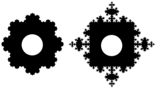
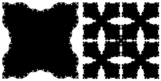
Let X be a Brownian motion. If X is killed on $\partial E$, we notice that ${\mathbf{E}}_x\left[\zeta \right]<\infty$. We underline the fact that if X is reflected on $\partial E\setminus \partial B$ and killed on $\partial B$ with $B\subset E$, we have that ${sup}_x{\mathbf{E}}_x\left[\zeta \right]<\infty$ only if E is non-trap for X. Examples of non-trap domains are given by smooth domains and snowflakes domains as the scale irregular (Koch) fractals in Figure 1 and Figure 2 (see [30] for details). Figure 1 and Figure 2 are realizations of the random domain obtained by randomly choosing the contraction factor step by step in the construction of the pre-fractals.

Figure 1. Koch curves outside the square. We have Neumann condition on $\partial E\setminus \partial B$ and Dirichlet condition on $\partial B$, where B is the Ball inside E. The domains are non-trap for the Brownian motion.

Figure 2. Koch curves inside the square. We have the Dirichlet condition on the boundary $\partial E$. The domains are non-trap for the Brownian motion.

Theorem 2.

([29]) Let Φ be the Bernstein function in (2). Let H be the subordinator with symbol Φ. We have:

$$\begin{array}{c}\hfill {\mathbf{E}}_x\left[{\zeta }^L\right]={\mathbf{E}}_x\left[H_{\zeta }\right],x\in E.\end{array}$$

(24)

Theorem 3.

([29]) Let Φ be the Bernstein Function (2). Let L be the inverse to a subordinator H with symbol Φ. We have that

$$\begin{array}{c}\hfill {\mathbf{E}}_x\left[{\zeta }^H\right]={\mathbf{E}}_x\left[L_{\zeta }\right],x\in E.\end{array}$$

(25)

The previous results must be read by considering that

$${\mathbf{E}}_x\left[H_{\zeta }\right]=\underset{\lambda \downarrow 0}{lim}\frac{\Phi \left(\lambda \right)}{\lambda }{\mathbf{E}}_x\left[\zeta \right]$$

(26)

whereas ${\mathbf{E}}_0\left[L_t\right]$ is known only in some cases (see, for example, [24]).

The time change may lead to an unexpected situation. The gamma subordinator represents a nice example in this direction. Let H be characterized by $\Phi \left(\lambda \right)=aln(1+\lambda /b)$ with $0<a,b<\infty$. Then, $\Phi \left(\lambda \right)/\lambda \to b/a$ for $\lambda \downarrow 0$, as mentioned above. This means that, for $b<a$, for example, the base process X is rushed by L and the process $X^L$ cannot be considered as a delayed process. We have a delaying effect for $b>a$. The process $X^L$ is actually a delayed process in case L is an inverse to a stable subordinator (with $\Phi \left(\lambda \right)={\lambda }^{\alpha }$). Indeed, the lifetime ${\zeta }^L$ turns out to be finite with some probability, but its mean value is infinite. Definition 2 must be therefore understood by considering all possible paths of a time-changed process. This means that we have processes “delayed in mean” or “rushed in mean”.

4. An Irregular Domain

Our aim is to underline some relation between non-local operators and the “regularity” of the domains. Such a connection is given in terms of stochastic processes describing the motions in those domains. In order to be clear, we present here a discussion based on a simple and instructive case, the fractal Koch domain.

4.1. Random Koch Domains (RKD)

Let ${\ell }_a\in (2,4)$ with $a\in I\subset \mathbb{N}$ be the reciprocal of the contraction factor for the family ${\Psi }^{\left(a\right)}$ of contractive similitudes ${\psi }_i^{\left(a\right)}:\mathbb{C}\to \mathbb{C}$ given by:

$$\begin{array}{c}\hfill {\psi }_1^{\left(a\right)}\left(z\right)=\frac{z}{{\ell }_a},{\psi }_2^{\left(a\right)}\left(z\right)=\frac{z}{{\ell }_a}{e}^{ı\theta \left({\ell }_a\right)}+\frac{1}{{\ell }_a},\end{array}$$

$$\begin{array}{c}\hfill {\psi }_3^{\left(a\right)}\left(z\right)=\frac{z}{{\ell }_a}{e}^{ı\theta \left({\ell }_a\right)}+\frac{1}{2}+ı\sqrt{\frac{1}{{\ell }_a}-\frac{1}{4}},{\psi }_4^{\left(a\right)}\left(z\right)=\frac{z-1}{{\ell }_a}+1\end{array}$$

where $\theta \left({\ell }_a\right)=arcsin(\sqrt{{\ell }_a(4-{\ell }_a)}/2)$. Let $\Xi =I^{\mathbb{N}}$ with $I\subset \mathbb{N}$, $\left|I\right|=N$, and let $\xi =({\xi }_1,{\xi }_2,\dots )\in \Xi$. We call $\xi$ an environment sequence, where ${\xi }_n$ says which family of contractive similitudes we are using at level n. Set ${\ell }^{\left(\xi \right)}\left(0\right)=1$ and

$$\begin{array}{c}\hfill {\ell }^{\left(\xi \right)}\left(n\right)=\prod _{i=1}^n{\ell }_{{\xi }_i}.\end{array}$$

We define a left shift S on $\Xi$ such that if $\xi =\left({\xi }_1,{\xi }_2,{\xi }_3,\dots \right),$ then $S\xi =\left({\xi }_2,{\xi }_3,\dots \right).$ For $B\subset {\mathbb{R}}^2$ set ${{\rm Y}}^{\left(a\right)}\left(B\right)={\bigcup }_{i=1}^4{\psi }_i^{\left(a\right)}\left(B\right)$ and ${{\rm Y}}_n^{\left(\xi \right)}\left(B\right)={{\rm Y}}^{\left({\xi }_1\right)}\circ \cdots \circ {{\rm Y}}^{\left({\xi }_n\right)}\left(B\right)$. The fractal $K^{\left(\xi \right)}$ associated with the environment sequence $\xi$ is defined by

$$K^{\left(\xi \right)}=\overline{\bigcup _{n=1}^{+\infty }{{\rm Y}}_n^{\left(\xi \right)}(\Gamma )}$$

where $\Gamma =\{P_1,P_2\}$ with $P_1=(0,0)$ and $P_2=(1,0).$ For $\xi \in \Xi ,$ we define the word space $W=W^{\left(\xi \right)}=\{(w_1,w_2,\dots ):1⩽w_i⩽4\}$, and for $w\in W,$ we set $w|n=(w_1,\dots ,w_n)$ and ${\psi }_{w|n}={\psi }_{w_1}^{\left({\xi }_1\right)}\circ \cdots \circ {\psi }_{w_n}^{\left({\xi }_n\right)}.$ The volume measure ${\mu }^{\left(\xi \right)}$ is the unique Radon measure on $K^{\left(\xi \right)}$ such that

$${\mu }^{\left(\xi \right)}({\psi }_{w|n}(K^{\left(S^n\xi \right)}))=\frac{1}{4^n}$$

for all $w\in W,$ as, for each $a\in A,$ the family ${\Psi }^{\left(a\right)}$ has four contractive similitudes. Let $K_0$ be the line segment of unit length with $P_1=(0,0)$ and $P_2=(1,0)$ as endpoints. We set, for each $n\in \mathbb{N}$,

$$K_n^{\left(\xi \right)}={{\rm Y}}_n^{\left(\xi \right)}\left(K_0\right)$$

and $K_n^{\left(\xi \right)}$ is the so-called n-th prefractal (deterministic) curve.

Let us consider the random vector $\mathit{\xi }=({\mathit{\xi }}_1,{\mathit{\xi }}_2,\dots )$, whose components ${\mathit{\xi }}_i$ take values on I with probability mass function $\mathbf{P}:\Xi \to [0,1]$. Thus, the construction of the random n-th pre-fractal curve $K_n^{\left(\mathit{\xi }\right)}={{\rm Y}}_n^{\left(\mathit{\xi }\right)}\left(K_0\right)$ depends on the realization of $\mathit{\xi }$ with probability $P({\mathit{\xi }}_i={\xi }_i)$ for its i-th component. We assume that ${\left\{{\mathit{\xi }}_i\right\}}_{i=1,\dots ,n}$ are identically distributed and ${\mathit{\xi }}_i\perp {\mathit{\xi }}_j$ for $i\ne j$; that is, we obtain the curve $K_n^{\left(\xi \right)}$ with probability

$$\begin{array}{c}\hfill \mathbf{P}\left(\mathit{\xi }\right|n=\xi \left|n\right)=\prod _{i=1}^n\mathbf{P}({\mathit{\xi }}_i={\xi }_i)\end{array}$$

where $\mathit{\xi }|n=({\mathit{\xi }}_1,\dots ,{\mathit{\xi }}_n)$ and $\xi |n=({\xi }_1,\dots ,{\xi }_n)$. Further on, we only use the superscript $\left(\xi \right|n)$ or $\left(\mathit{\xi }\right|n)$ in order to streamline the notation.

Given the random environment sequence $\mathit{\xi }$, the random fractal $K^{\left(\mathit{\xi }\right)}$ is therefore defined by the deterministic fractal $K^{\left(\xi \right)}$.

Let ${\Omega }^{\left(\xi \right|n)}$ be the planar domain obtained from a regular polygon by replacing each side with a pre-fractal curve $K_n^{\left(\xi \right)}$ and ${\Omega }^{\left(\xi \right)}$ be the planar domain obtained by replacing each side with the corresponding fractal curve $K^{\left(\xi \right)}$. We introduce the random planar domains ${\Omega }^{\left(\mathit{\xi }\right|n)}$ and ${\Omega }^{\left(\mathit{\xi }\right)}$ by considering the random curves $K_n^{\left(\mathit{\xi }\right)}$ and $K^{\left(\mathit{\xi }\right)}$. Examples of (pre-fractal) random Koch domains are given in Figure 3 (outward curves), Figure 4 (inward curves) and Figure 5 (inward curves) by choosing the square as the regular polygon.

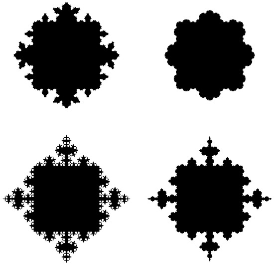
Figure 3. Outward curves.

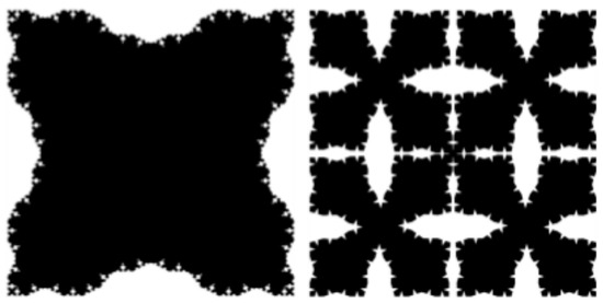
Figure 4. Inward curves.

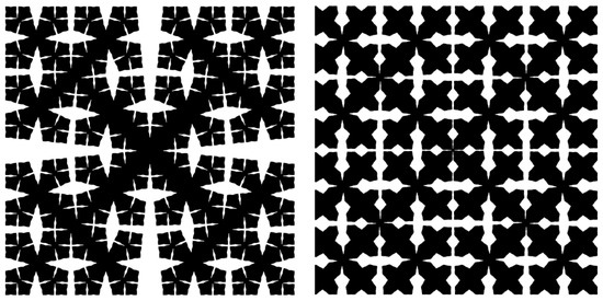
Figure 5. Inward curves.

Theorem 4.

For the sequence of (random) Hausdorff dimensions $d^{\left(\mathit{\xi }\right|n)}$, we have that

$$\begin{array}{c}\hfill d^{\left(\mathit{\xi }\right|n)}\stackrel{a.s.}{\to }{d}^{\left(\mathit{\xi }\right)}=\frac{ln4}{\mathbf{E}[ln{\ell }_{{\mathit{\xi }}_1}]},n\to \infty .\end{array}$$

Proof. 

Since ${\mathit{\xi }}_i\stackrel{law}{=}{\mathit{\xi }}_1$, $\forall i$, we have that the Hausdorff dimension $d^{\left(\mathit{\xi }\right)}$ of the curve $K^{\left(\mathit{\xi }\right)}$ can be obtained by considering the strong law of large numbers and the fact that

$$\begin{array}{c}\hfill \frac{ln{4}^n}{{\sum }_{i=1}^n{\ell }_{{\mathit{\xi }}_i}}=\frac{ln4}{\frac{1}{n}{\sum }_{i=1}^n{\ell }_{{\mathit{\xi }}_i}}\stackrel{a.s.}{\to }\frac{ln4}{\mathbf{E}[ln{\ell }_{{\mathit{\xi }}_1}]},n\to \infty .\end{array}$$

Then (see [31] (Lemma 2.3)),

$$\begin{array}{c}\hfill d^{\left(\mathit{\xi }\right)}=\frac{ln4}{ln{\prod }_{a\in I}{\left({\ell }_a\right)}^{P({\mathit{\xi }}_1=a)}}=\frac{ln4}{\mathbf{E}[ln{\ell }_{{\mathit{\xi }}_1}]}.\end{array}$$

(27)

□

The measure ${\mu }^{\left(\xi \right)}$ satisfies the following property. There exist two positive constants, $C_1,C_2,$ such that

$$C_1{r}^{d^{\left(\xi \right)}}\le {\mu }^{\left(\xi \right)}(\mathcal{B}(P,r)\cap K^{\left(\xi \right)})\le C_2{r}^{d^{\left(\xi \right)}},\forall P\in K^{\left(\xi \right)},$$

(28)

where $\mathcal{B}(P,r)$ denotes the Euclidean ball with a center in P and radius $0<r\le 1$ (see [31]). According to Jonsson and Wallin [32], we say that $K^{\left(\xi \right)}$ is a d-set with respect to the Hausdorff measure ${\mathcal{H}}^d,$ with $d=d^{\left(\xi \right)}.$ The sequence

$$\begin{array}{c}\hfill {\sigma }^{\left(\xi \right|n)}=\frac{{\ell }^{\left(\xi \right|n)}}{4^n},\mathrm{where}{\ell }^{\left(\xi \right|n)}=\prod _{i=1}^n{\ell }_{{\xi }_i}\end{array}$$

(29)

is obtained from the realization of $\mathit{\xi }|n$ and, therefore, from the realization of the random variable ${\ell }^{\left(\mathit{\xi }\right|n)}$ with mean value given by

$$\begin{array}{c}\hfill \mathbf{E}\left[{\ell }^{\left(\mathit{\xi }\right|n)}\right]=\prod _{i=1}^n\mathbf{E}\left[{\ell }_{{\mathit{\xi }}_i}\right]={\left(\mathbf{E}\left[{\ell }_{{\mathit{\xi }}_1}\right]\right)}^n.\end{array}$$

For $\alpha =\mathbf{E}{\ell }_{{\mathit{\xi }}_1}\in (2,4)$, we find the mean value $\mathbf{E}\left[{\sigma }^{\left(\mathit{\xi }\right|n)}\right]={\alpha }^n/4^n$ from (29). In terms of that sequence, we are able to deal with the pre-fractal (and fractal) boundary by introducing, for example, the Revuz measure associated with some boundary functional. In particular, we take into account the integral

$$\begin{array}{c}\hfill {\sigma }^{\left(\xi \right|n)}{\int }_{\partial {\Omega }^{\left(\xi \right|n)}}f\left(x\right){\mathbf{1}}_{\Lambda }\left(x\right)d\mathfrak{s},\Lambda \in \partial {\Omega }^{\left(\xi \right|n)},n\in \mathbb{N}\end{array}$$

where $\mathfrak{s}$ is the arc-length measure on the pre-fractal boundary leading to the Hausdorff measure ${\mu }^{\left(\xi \right)}$ on the fractal boundary, as $n\to \infty$, ${\sigma }^{\left(\xi \right|n)}$ ensures convergence.

The random contraction factors give rise to random (pre-fractal) Koch domains ${\Omega }^{\left(\mathit{\xi }\right|n)}$. The random (fractal) Koch domains ${\Omega }^{\left(\mathit{\xi }\right)}$ are obtained as described above. In order to gain a clear picture of the relevance of the Koch domain in our analysis, we recall an example introduced in [28]. Assume that the construction of a Koch curve $K^{\left(\xi \right)}$ is given by the picture in Figure 6. The Koch domain becomes a trap domain for the Brownian motion according with the asymptotic behavior of the opening size.

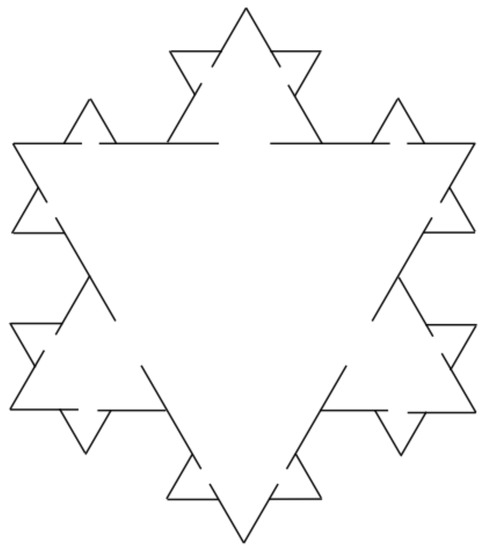
Figure 6. The modified Koch domain (pre-fractal, second step) introduced in [28]. The passage between triangles is blocked by a wall with a small opening. The construction can be considered for random Koch domains. The time the process spends in a triangle strongly depends on the size of the opening. The asymptotic behavior of that size implies the construction of trap or non-trap Koch domains.

4.2. Non-Local Initial Value Problem on the RKD

In [33], we consider the sequence of time-changed process $X^{L,n}=X^n\circ L$, where $X^n$ is an elastic Brownian motion on ${\Omega }^{\left(\mathit{\xi }\right|n)}$ with elastic coefficient $c_n$. We study the asymptotic behavior of $X^{L,n}$ depending on the asymptotics for $c_n$. In the deterministic case, the process $X^{L,n}$ can be associated with the non-local Cauchy problem on ${\Omega }^{\left(\xi \right|n)}$:

$$\begin{array}{c}\hfill {\mathfrak{D}}_t^{\Phi }u=A^{n}u,u_0=f\in D\left(A^n\right).\end{array}$$

Denote by $\mathbb{D}$ the set of continuous functions from $[0,\infty )$ to $E_{\partial }={\Omega }^{\left(\xi \right)}\cup \partial$ which are right continuous on $[0,\infty )$ with left limits on $(0,\infty )$. Here, ∂ is the cemetery point, that is, $E_{\partial }^n$ is the one-point compactification of $E^n={\Omega }^{\left(\xi \right|n)}$, $n\in \mathbb{N}$. Denote by ${\mathbb{D}}_0$ the set of non-decreasing continuous functions from $[0,\infty )$ to $[0,\infty )$. Let X be the process on the random fractal ${\Omega }^{\left(\mathit{\xi }\right)}$ with generator $(A,D(A\left)\right)$, where A is the Neumann, the Dirichlet or the Robin Laplacian if $c_n\to c$ with $c=0,\infty$ or a constant.

Theorem 5.

([33]) As $n\to \infty$,

$$\begin{array}{c}\hfill X^{L,n}\to X^L\mathit{in}\mathit{distribution}\mathit{in}\mathbb{D}\mathit{\xi }-a.s.\mathit{on}{\Omega }^{\left(\mathit{\xi }\right)}.\end{array}$$

This result says that we have a time-change representation for the solution to the non-local Cauchy problem on the (fractal) Koch snowflakes.

The Koch domain (as the random Koch domain) is quite regular in a sense to be better explained. Under Definition 1, Koch domains are non-trap for the Brownian motion, and therefore, we may say that the boundary $\partial {\Omega }^{\left(\mathit{\xi }\right)}$ is regular.

5. Non-Local Boundary Value Problems

5.1. Singular Kernels

For a bounded subset $\Omega$ of ${\mathbb{R}}^d$, we first focus on the fractional boundary value problem:

$$\begin{array}{c}\hfill \left\{\begin{array}{c}{\displaystyle \frac{\partial u}{\partial t}(t,x)=\Delta u(t,x),t>0,x\in \Omega }\hfill \\ \\ {\displaystyle \eta D_t^{\alpha }u(t,x)+\sigma {\partial }_{\mathbf{n}}u(t,x)+cu(t,x)=0,t>0,x\in \partial \Omega }\hfill \\ \\ {\displaystyle u(0,x)=f\left(x\right),x\in \overline{\Omega }}\hfill \end{array}\right.\end{array}$$

(30)

where $\eta ,\sigma ,c$ are positive constants, $\alpha \in (0,1)$, ${\partial }_{\mathbf{n}}u$ is the outer normal derivative and $D_t^{\alpha }u(t,x)$ is the Caputo–Dzherbashian fractional derivative. As before, we write $u_f=u_f(t,x)$ for the function such that

$$\begin{array}{c}\hfill u_f\to f\mathrm{as}t\downarrow 0.\end{array}$$

Then, we introduce the space

$$\begin{array}{c}\hfill D_L=\left\{\phi ={\phi }_{{f|}_{\partial \Omega }}:\left|\frac{\partial \phi }{\partial t}(t,x)\right|\le v\left(x\right)t^{\alpha -1},v\in L^{\infty }(\partial \Omega )\right\}.\end{array}$$

We also introduce the processes $\overline{X}={\left\{{\overline{X}}_t\right\}}_{t\ge 0}$ and $\widehat{X}={\{{\widehat{X}}_t\}}_{t\ge 0}$ defined as follows. Let $X={\left\{X_t\right\}}_{t\ge 0}$ be a Brownian motion on $\overline{\Omega }=\Omega \cup \partial \Omega$, where $\Omega$ is a bounded subset of ${\mathbb{R}}^d$. Let $L={\left\{L_t\right\}}_{t\ge 0}$ be an inverse to an $\alpha$-stable subordinator $H={\left\{H_t\right\}}_{t\ge 0}$. Define the time-changed process $\widehat{X}={\{{\widehat{X}}_t\}}_{t\ge 0}$ as the composition $\widehat{X}:=X\circ \widehat{L}$ with ${\widehat{L}}_t=t$ if $\widehat{X}$ is running on $\Omega$ and ${\widehat{L}}_t=L_t$ if $\widehat{X}$ is on $\partial \Omega$. Furthermore, we define $\overline{X}$ as the composition of an elastic Brownian motion (Robin boundary condition for the associated Cauchy problem) and the inverse to the process

$$\begin{array}{c}\hfill {\overline{V}}_t=t+H\circ (\eta /\sigma ){\gamma }_t\end{array}$$

where $\gamma ={\left\{{\gamma }_t\right\}}_{t\ge 0}$ is the local time on $\partial \Omega$ of the reflecting Brownian motion $X^{+}$ on $\overline{\Omega }$. We recall that an elastic Brownian motion can be written by considering the couple $(X^{+},\gamma )$.

We have the following result.

Theorem 6.

([34]) For the solution $u\in C^{1,2}((0,\infty ),\overline{\Omega })\cap D_L$ to the fractional boundary value problem (30), we have that:

(i) 

The solution is given by:

$$\begin{array}{c}\hfill u(t,x)={\int }_{\overline{\Omega }}f\left(y\right)\left({\int }_{0}p(s,x,y)l(t,s;y)ds\right)m\left(dy\right),t>0,x\in \overline{\Omega }\end{array}$$

(31)

with the probabilistic representation

$$\begin{array}{c}\hfill u(t,x)={\mathbf{E}}_x[f({\widehat{X}}_t)],t>0,x\in \overline{\Omega };\end{array}$$

(32)

(ii) 

Moreover, the following representation holds true:

$$\begin{array}{cc}\hfill u(t,x)=& {\mathbf{E}}_x\left[f\left({\overline{X}}_t\right)\right]\hfill \\ \hfill =& {\mathbf{E}}_x\left[f(X^{+}\circ {\overline{V}}_t^{-1})exp\left(-(c/\sigma )\gamma \circ {\overline{V}}_t^{-1}\right)\right],t>0,x\in \overline{\Omega }\hfill \end{array}$$

(33)

where ${\overline{V}}_t^{-1}$ is the inverse to ${\overline{V}}_t=t+H\circ (\eta /\sigma ){\gamma }_t$. The process $\overline{X}={\left\{{\overline{X}}_t\right\}}_{t\ge 0}$ can be constructed as a time-changed elastic Brownian motion.

The previous results give a clear picture about the boundary behavior of the associated process near the boundary. In particular, by considering the representation in terms of $\overline{X}$, since the process H may have jumps, then the inverse to ${\overline{V}}_t$ slows down the process on the boundary according with the plateaus associated with those jumps (see Figure 7). As $\alpha =1$, the process ${\overline{V}}_t$ becomes $V_t=t+(\eta /\sigma ){\gamma }_t$, and $\overline{X}$ corresponds to the elastic sticky Brownian motion. An interesting description in terms of excursions and waiting times can be given as in Figure 8.

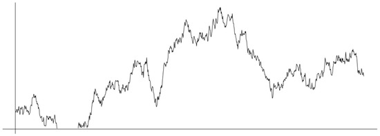
Figure 7. The 1-dimensional path (a realization of $\widehat{X}$ or $\overline{X}$) exhibits a trap effect at zero. The process stops for a random amount of time (according with ${\overline{V}}^{-1}$); then, it reflects continuously. The same effect can be considered on the boundary $\partial \Omega$ for d-dimensional motions with random time-change ${\overline{V}}^{-1}$.

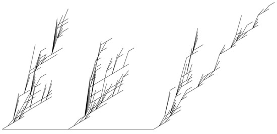
Figure 8. Graphs in a forest in which the distances are randomly determined by ${\overline{V}}^{-1}$. Each graph represents an excursion of $\overline{X}$ in the sense of Lukasiewicz path with a rotation for the edges of each vertex in order to obtain the (more attractive) Lichtenberg figures. The waiting time at zero gives the random distance between Lightning graphs.

The fractional boundary value problem above introduces independent waiting times on the boundary $\partial \Omega$ in terms of $\overline{V}$. This means that a given stop can be explained by an endogenous effect. We exploit such a reading in order to provide a connection with trap boundaries.

For example, the process $\overline{X}$ on a (non-trap) Koch domain can be considered in order to describe the motion of a Brownian motion $B^{+}$ on a (trap) Koch domain obtained as in Figure 6.

In the papers [34,35], the lifetime of the process $\overline{X}$ has been investigated together with an interesting connection with irregular domains. In particular, the time the process spends on the boundary can be related with a delayed reflection or an irregular boundary as well. The non-local boundary value problem (for a smooth domain) can be therefore associated with a local boundary value problem (for an irregular domain).

A further result concerning non-local boundary conditions has been investigated in [25]. We provide here only the main idea. Let $D_0=D_1\cup D_2$ be the set given by considering the sets:

$$\begin{array}{c}\hfill D_1=\left\{\phi :\forall x>0,\phi (·,x)\in W^{1,\infty }(0,\infty )\mathrm{and}\forall t>0,\underset{x\downarrow 0}{lim}{\mathfrak{D}}_t^{\Psi }\phi (t,x)\mathrm{exists}\right\}\end{array}$$

and

$$\begin{array}{c}\hfill D_2=\left\{\phi :\forall t>0,\phi (t,·)\in W^{1,\infty }(0,\infty )\mathrm{and}\forall t>0,\underset{x\downarrow 0}{lim}{\mathbf{D}}_{x+}^{\Phi }\phi (t,x)\mathrm{exists}\right\}.\end{array}$$

Then, we state the following result concerning the problem:

$$\left\{\begin{array}{cc}{\displaystyle \frac{\partial u}{\partial t}(t,x)=\frac{{\partial }^{2}u}{\partial x^2}(t,x),}\hfill & t>0,x\in (0,\infty )\hfill \\ \\ {\displaystyle \eta {\mathfrak{D}}_t^{\Psi }u(t,0)+\sigma {\mathbf{D}}_{x+}^{\Phi }u(t,0)=0,}\hfill & t>0\hfill \\ \\ {\displaystyle u(0,x)=f\left(x\right),}\hfill & x\in [0,\infty )\hfill \end{array}\right.$$

(34)

for an initial datum $f\in C[0,\infty )\cap L^{\infty }(0,\infty )$ and positive constants $\eta ,\sigma$.

Theorem 7.

([25]) For the solution $u\in C^{1,2}((0,\infty ),(0,\infty ))\cap D_0$ to the problem (34), we have the following probabilistic representation:

$$\begin{array}{c}\hfill u(t,x)={\mathbf{E}}_x\left[X_t^{•}\right]={\mathbf{E}}_x[f(X^{+}\circ {\overline{V}}_t^{-1}+R_{\gamma }\circ {\overline{V}}_t^{-1})],t>0,x\in [0,\infty )\end{array}$$

where

-

The couple $(X^{+},\gamma )$ has been defined above;

-

${\overline{V}}_t^{-1}$ is an inverse as defined in the previous theorem with $H=H^{\Psi }$;

-

$R_t=H\circ L_t-t$ is the composition of a subordinator and its inverse with $H=H^{\Phi }$.

A detailed discussion on the path behavior of that process is given in [25]. The process near the boundary jumps inside the domain because of $R_t$, and then it stops there according to ${\overline{V}}_t^{-1}$ (see Figure 9). Here, we recall that a subordinator can be obtained from a compound Poisson process (see [36]), written as:

$$\begin{array}{c}\hfill \frac{1}{n}\sum _{k=1}^{N_{nt}}{ϵ}_k{e}^{{\chi }_k},t>0,n\in \mathbb{N}\end{array}$$

where $N_t$ is a Poisson process, and ${\chi }_k$ are exponential random variables such that $\mathbf{P}({\chi }_k>x)=e^{-\alpha x}$ and $\mathbf{P}({ϵ}_k=1)=1$. The case in which $\mathbf{P}({ϵ}_k=+1)=p$ and $\mathbf{P}({ϵ}_k=-1)=q$ leads to the limit $H_{pt}-H_{qt}$ as $n\to \infty$. Concerning our case, we can approximate the last jump of H given by R by considering the jump $Y_k={ϵ}_k{e}^{{\chi }_k}$ with power law $P(Y_k\in dy)=\alpha n^{-\alpha }{y}^{-\alpha -1}{\mathbf{1}}_{(y>1/n)}dy$. The jump never occur if its length is less than a given threshold.

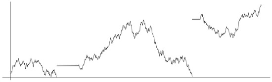
Figure 9. The path of $X^{+}\circ {\overline{V}}_t^{-1}+R_{\gamma }\circ {\overline{V}}_t^{-1}$. The process exhibits a jump and stop behavior near the boundary. Indeed, the process never hits the zero point boundary; it jumps near the boundary according to $R_{\gamma }$, and then it stops for a random amount of time according to ${\overline{V}}^{-1}$.

In case ${\mathbf{D}}_{x+}^{\Phi }$ is written in terms of a non-singular kernel, the jumps can be well-described, as in the next section, and the process $R_t$ can be associated with a compound Poisson process. This boundary behavior with jumps has been first investigated in [37,38] with no mention about non-local operators which have been considered in [25]. The novelty concerned with random holding time at the boundary has been first treated in [34,35] by extending the sticky boundary condition introduced by Feller in [39] and Wentzell in [40] with the probabilistic representation in terms of sample paths obtained by Itô and McKean ([38], Section 10).

The connection between the local and non-local boundary value problems seems to be quite intriguing. Consider the problems:

$$\left\{\begin{array}{cc}{\displaystyle \frac{\partial u}{\partial t}(t,x)=\mu \frac{\partial u}{\partial x}(t,x)+\frac{{\partial }^{2}u}{\partial x^2}(t,x),}\hfill & t>0,x\in (0,\infty )\hfill \\ \\ {\displaystyle \frac{\partial u}{\partial x}(t,0)=c_{0}u(t,0),}\hfill & t>0\hfill \\ \\ {\displaystyle u(0,x)=f\left(x\right),}\hfill & x\in [0,\infty )\hfill \end{array}\right.$$

(35)

and

$$\left\{\begin{array}{cc}{\displaystyle \frac{\partial u}{\partial t}(t,x)=\mu \frac{\partial u}{\partial x}(t,x)+\frac{{\partial }^{2}u}{\partial x^2}(t,x),}\hfill & t>0,x\in (0,\infty )\hfill \\ \\ {\displaystyle {\mathfrak{D}}_t^{\Phi }u(t,0)+c_{1}u(t,0)=c_2,}\hfill & t>0\hfill \\ \\ {\displaystyle u(0,x)=f\left(x\right),}\hfill & x\in [0,\infty )\hfill \end{array}\right.$$

(36)

where $\Phi \left(\lambda \right)=\sqrt{\lambda +{(\mu /2)}^2}-\sqrt{{(\mu /2)}^2}$ introduces the so-called tempered derivative (of Caputo–Dzherbashian type). For the sake of simplicity, here we consider $c_0$, $c_1$, $c_2$ as given constants. In [41], starting from a previous result in [42], it has been shown that the solution coincides in case f is constant. Thus, for the elastic drifted Brownian motion, say $X_t^{\mu ,c_0}$, we can write:

$$\begin{array}{c}\hfill u(t,x)={\mathbf{E}}_x\left[f\left(X_t^{\mu ,c_0}\right)M_t^{\mu ,c_0}\right]\end{array}$$

where the multiplicative functional associated with the elastic condition can be written in terms of L, the inverse to a subordinator H with symbol $\Phi$. In particular, $M^{\mu ,c_0}$ is equivalent to ${\overline{M}}^{c_1,c_2}={\overline{M}}^{c_1,c_2}\left(L\right)$, which is associated with the non-local (tempered) boundary condition.

In the literature, some works deal with non-local boundary value problems with different meaning (see, for example, [43,44,45]). Our approach is motivated by the clear effort to find a description for anomalous behavior near smooth boundaries with possible application in case of irregular boundaries.

5.2. Non-Singular Kernels

We focus on a famous operator which has been deeply discussed in the last few years. Recently, in a series of papers starting from [46], some authors considered the Caputo–Fabrizio operator (for a given constant a):

$$\begin{array}{c}\hfill {\mathcal{D}}_x^{\left(\alpha \right)}u\left(x\right)=\frac{M\left(\alpha \right)}{1-\alpha }{\int }_a^x{u}^{\prime }\left(\tau \right)exp\left[-\frac{\alpha (x-\tau )}{1-\alpha }\right]d\tau \end{array}$$

where $M\left(\alpha \right)$ is a normalizing function such that $M\left(0\right)=M\left(1\right)=1$, and $\alpha \in (0,1)$ is the fractional order of the operator. The operator has been introduced as a fractional derivative, although the proper definition of fractional operators is now stimulating a deep debate [47]. However, the operator ${\mathcal{D}}_x^{\left(\alpha \right)}$ can be regarded as a non-singular operator and can be included in the class of integro-differential operators. As pointed out in [46], we have that ${\mathcal{D}}_x^{\left(\alpha \right)}u\left(x\right)\to u^{\prime }\left(x\right)$ as $\alpha \to 1$ and ${\mathcal{D}}_t^{\left(\alpha \right)}u\left(x\right)\to u\left(x\right)-u\left(a\right)$ as $\alpha \to 0$. For the sake of simplicity, we assume here that $a=0$ and $u\left(0\right)=0$. Our results are concerned with the boundary value problem in which the boundary-operator

$$\begin{array}{c}\hfill {\mathcal{D}}_x^{\left(\alpha \right)}u+c\alpha u=0,c\ge 0\end{array}$$

(37)

is considered. As a consequence of the properties illustrated before for the Caputo–Fabrizio operator as $\alpha \to 0$ or $\alpha \to 1$, we have

$$\begin{array}{c}\hfill u\left(x\right)=0\mathrm{or}{u}^{\prime }\left(x\right)=-cu\left(x\right),\end{array}$$

(38)

respectively, in place of (37). The conditions (38) correspond to Dirichlet or Robin conditions, respectively. For $\alpha \in [0,1]$ and $c\ge 0$, we consider the solution to

$$\begin{array}{c}\hfill \frac{\partial u}{\partial t}=Gu,u_0=f\end{array}$$

with

$$\begin{array}{c}\hfill ({\mathcal{D}}_x^{\left(\alpha \right)}u+c\alpha u){|}_{x=0}=0\end{array}$$

where G is the generator of a Markov process on $[0,\infty )$.

In [46], the authors provided some properties of ${\mathcal{D}}_x^{\left(\alpha \right)}u\left(x\right)$. For $a=0$ for instance, the Laplace transform reads as follows (as usual, we denote by $\tilde{u}$ the Laplace transform of u)

$$\begin{array}{cc}\hfill {\int }_0^{\infty }{e}^{-\lambda x}{\mathcal{D}}_x^{\left(\alpha \right)}u\left(x\right)dx=& \frac{M\left(\alpha \right)}{1-\alpha }\left(\lambda \tilde{u}\left(\lambda \right)-u\left(0\right)\right){\int }_0^{\infty }{e}^{-\lambda x}{e}^{-\frac{\alpha x}{1-\alpha }}dx\hfill \\ \hfill =& M\left(\alpha \right)\frac{1}{\alpha +\lambda (1-\alpha )}\left(\lambda \tilde{u}\left(\lambda \right)-u\left(0\right)\right).\hfill \end{array}$$

(39)

From now on, we assume that

$$\begin{array}{c}\hfill M\left(\alpha \right)=1\mathrm{and}a=0.\end{array}$$

(40)

The Laplace transform (39) corresponds to the Laplace transform of the fractional operator ${\mathfrak{D}}_x^{\Phi }$ with Lèvy symbol and measure

$$\begin{array}{c}\hfill \Phi \left(\lambda \right)=(\theta +1)\frac{\lambda }{\theta +\lambda }\mathrm{and}\overline{\varphi }\left((y,\infty )\right)=(\theta +1)e^{-\theta y},\theta =\frac{\alpha }{1-\alpha }\end{array}$$

(41)

where, as a quick check shows,

$$\begin{array}{c}\hfill \underset{\lambda \downarrow 0}{lim}\frac{\Phi \left(\lambda \right)}{\lambda }=\frac{1}{\alpha }.\end{array}$$

From a probability view-point, the symbol $\Phi$ characterizes a subordinator H, that is, a non-negative, non-decreasing process. Notice that $\overline{\varphi }\left((0,\infty )\right)<\infty$ if $\alpha <1$, and the process $H_t$ is a step-process: its trajectories are not strictly increasing. The inverse to a subordinator can be defined as:

$$\begin{array}{c}\hfill L_t=inf\{s\ge 0:H_s>t\},t>0\end{array}$$

from which we also obtain the relation:

$$\begin{array}{c}\hfill {\mathbf{P}}_0(H_t<x)={\mathbf{P}}_0(L_x>t),x,t>0.\end{array}$$

(42)

As $\alpha \to 1$, we obtain $\Phi \left(\lambda \right)=\lambda$ as expected, and the process H corresponds to the elementary subordinator $H_t=t$. We recall that $L_t$ may have plateaus only if the process $H_t$ may have jumps (at least for $\alpha \ne 1$). Since $H_t$ has non-decreasing paths, the inverse $L_t$ may have jumps (L is not continuous). Thus, H is not strictly increasing, and $L_t$ cannot be continuous. As $\alpha \to 0$, the ratio $\Phi \left(\lambda \right)/\lambda$ gives an infinite mean life time and therefore a delayed process on the boundary. This actually corresponds to an absorption at $x=0$, whereas the Dirichlet condition suggests a kill. We still have [3]:

$$\begin{array}{c}\hfill {\mathbf{E}}_0\left[{\int }_0^{\infty }{e}^{-\lambda t}f\left(L_t\right)dt\right]=\frac{\Phi \left(\lambda \right)}{\lambda }{\mathbf{E}}_0\left[{\int }_0^{\infty }{e}^{-\lambda H_t}f\left(t\right)dt\right].\end{array}$$

(43)

Thus, for $f={\mathbf{1}}_D$ with $D\subseteq (0,\infty )$:

$$\begin{array}{c}\hfill {\int }_0^{\infty }{e}^{-\lambda t}{\mathbf{P}}_0(L_t\in D)dt=\frac{\Phi \left(\lambda \right)}{\lambda }{\int }_D{e}^{-t\Phi \left(\lambda \right)}dt.\end{array}$$

(44)

We also write:

$$\begin{array}{c}\hfill {\int }_0^{\infty }{e}^{-\lambda t}{\mathbf{P}}_0(L_t\in dx)dt=\frac{\Phi \left(\lambda \right)}{\lambda }{e}^{-x\Phi \left(\lambda \right)}dx\end{array}$$

and the density l of L solves:

$$\begin{array}{c}\hfill {\mathcal{D}}_t^{\left(\alpha \right)}l=-{\partial }_{x}l\end{array}$$

where L is an inverse of H with symbol $\Phi \left(\lambda \right)=(\theta +1)\frac{\lambda }{\theta +\lambda }$. It can be easily shown that H is a compound Poisson process. Indeed, consider the process

$$\begin{array}{c}\hfill H_t=\sum _{k=1}^{N_t}{Y}_k\end{array}$$

where $N_t\sim Pois\left((\theta +1)t\right)$ and $Y_k$ are i.i.d. random variables with $Y_1\sim Exp\left(\theta \right)$, $\theta >0$. For the reader’s convenience, we recall that, for $N_t\perp Y_1$,

$$\begin{array}{cc}\hfill \mathbf{E}\left[e^{-\lambda H_t}\right]=& \mathbf{E}\left[\prod _{k=1}^{N_t}{e}^{-\lambda Y_1}\right]=\mathbf{E}\left[{\left(\mathbf{E}\left[e^{-\lambda Y_1}\right]\right)}^{N_t}\right]\hfill \\ \hfill =& exp\left(-(\theta +1)t\left(1-\mathbf{E}\left[e^{-\lambda Y_1}\right]\right)\right).\hfill \end{array}$$

Thus, it turns out that

$$\begin{array}{c}\hfill \mathbf{E}\left[e^{-\lambda H_t}\right]=exp\left(-t(\theta +1){\int }_0^{\infty }(1-e^{-\lambda y})\theta e^{-\theta y}dy\right),\lambda >0.\end{array}$$

Our focus is on the boundary condition

$$\begin{array}{c}\hfill {\mathcal{D}}_x^{\left(\alpha \right)}u(t,0)+c\alpha u(t,0)=0\end{array}$$

corresponding to the drifted process $H_t+c\alpha t=:{\overline{H}}_t$. The process ${\overline{H}}_t$ may have jumps, never plateaus, except for $c=0$. This process is therefore strictly increasing with continuous inverse ${\overline{H}}_t^{-1}$, for which (see also [48]).

$$\begin{array}{c}\hfill \mathbf{P}({\overline{H}}_t^{-1}>s)=\mathbf{P}(t<{\overline{H}}_s)=\mathbf{P}(t-c\alpha s<H_s)\end{array}$$

and

$$\begin{array}{c}\hfill {\int }_0^{\infty }{e}^{-\lambda t}\mathbf{P}({\overline{H}}_t^{-1}>s)dt=\frac{1}{\lambda }{e}^{-s(c\alpha \lambda +(\theta +1)\frac{\lambda }{\theta +\lambda })},\lambda >0.\end{array}$$

By considering the symbol $\Phi \left(\lambda \right)=c\alpha \lambda +\frac{\theta +1}{\theta +\lambda }\lambda$, we have the (space) non-local boundary condition discussed in the previous section. The interested reader can also consult [49] for a discussion on this operator.

Many other cases can be considered. Indeed, the operator

$$\begin{array}{c}\hfill {\mathcal{D}}_x^{\Phi }u\left(x\right):={\int }_0^x{u}^{\prime }\mathcal{K}(x-\tau )d\tau \end{array}$$

(45)

with the non-singular kernel $\mathcal{K}$ can be associated with a compound Poisson process as above. Let us consider $\mathbf{P}(Y_k\in dy)=f_{Y_1}\left(y\right)dy$ for the jumps from the boundary, where $Y_k$ takes values in some set $supp\left(Y_k\right)=supp\left(f_{Y_1}\right)\subset (0,\infty )$. We do not consider negative jumps. Then, we obtain:

$$\begin{array}{c}\hfill \mathbf{E}\left[e^{-\lambda H_t}\right]=exp\left(-t(\theta +1){\int }_0^{\infty }\left(1-e^{-\lambda y}\right)f_{Y_1}\left(y\right)dy\right),\lambda >0\end{array}$$

and, for u such that $u\left(x\right)=0$ as $x\le 0$:

$$\begin{array}{cc}\hfill {\mathcal{D}}_x^{\Phi }u\left(x\right)=& (\theta +1){\int }_0^{\infty }\left(u\left(x\right)-u(x-y)\right)f_{Y_1}\left(y\right)dy\hfill \\ \hfill =& -(\theta +1){\int }_0^{\infty }{f}_{Y_1}\left(y\right){\int }_0^y\frac{du}{dz}(x-z)dzdy\hfill \\ \hfill =& -(\theta +1){\int }_0^{\infty }\frac{du}{dz}(x-z){\int }_z^{\infty }{f}_{Y_1}\left(y\right)dydz\hfill \\ \hfill =& (\theta +1){\int }_0^x{u}^{\prime }(x-z)\mathbf{P}(Y_1>z)dz.\hfill \end{array}$$

Thus, straightforward calculations lead to (45) with non-singular kernel

$$\begin{array}{c}\hfill \mathcal{K}\left(z\right)=(\theta +1)\mathbf{P}(Y_1>z),\theta >-1.\end{array}$$

A quick example is given by $Y_1$ distributed as a Mittag–Leffler random variable for which $\mathbf{P}(Y_1>y)=E_{\alpha }(-r{y}^{\alpha })$ with $r>0$ and $\alpha \in (0,1]$. It is well-known that for $\alpha =1$, we have $Y_1\sim Exp\left(r\right)$, obtaining the case discussed above.

References

- Bertoin, J. Subordinators: Examples and Applications. In Lectures on Probability Theory and Statistics. Lecture Notes in Mathematics; Bernard, P., Ed.; Springer: Berlin/Heidelberg, Germany, 1999; Volume 1717. [Google Scholar]
- D’Ovidio, M. On the fractional counterpart of the higher-order equations. Stat. Probab. Lett. 2011, 81, 1929–1939. [Google Scholar] [CrossRef]
- Capitanelli, R.; D’Ovidio, M. Fractional equations via convergence of forms. Fract. Calc. Appl. Anal. 2019, 22, 844–870. [Google Scholar] [CrossRef]
- Caputo, M. Elasticità e Dissipazione; Zanichelli: Bologna, Italy, 1969. [Google Scholar]
- Caputo, M.; Mainardi, F. Linear models of dissipation in anelastic solids. Riv. Nuovo C 1971, 1, 161–198. [Google Scholar] [CrossRef]
- Caputo, M.; Mainardi, F. A new dissipation model based on memory mechanism. Pure Appl. Geophys. 1971, 91, 134–147. [Google Scholar] [CrossRef]
- Dzherbashian, M.M. Integral Transforms and Representations of Functions in the Complex Plane; Nauka: Moscow, Russia, 1966. (In Russian) [Google Scholar]
- Dzherbashian, M.M.; Nersessian, A.B. Fractional derivatives and the Cauchy problem for differential equations of fractional order. Izv. Akad. Nauk. Armjan. SSR. Ser. Mat. 1968, 3, 1–29. (In Russian) [Google Scholar] [CrossRef]
- Ortigueira, M.D.; Machado, J.A.T. What is a fractional derivative? J. Comput. Phys. 2015, 293, 4–13. [Google Scholar] [CrossRef]
- Phillips, R.S. On the generation of semigroups of linear operators. Pac. J. Math. 1952, 2, 343–369. [Google Scholar] [CrossRef]
- Bochner, S. Diffusion equation and stochastic processes. Proc. Natl. Acad. Sci. USA 1949, 35, 368–370. [Google Scholar] [CrossRef]
- D’Ovidio, M.; Toaldo, B.; Orsingher, E. Time changed processes governed by space-time fractional telegraph equations. Stoch. Anal. Appl. 2014, 32, 1009–1045. [Google Scholar] [CrossRef][Green Version]
- D’Ovidio, M.; Toaldo, B.; Orsingher, E. Fractional telegraph-type equations and hyperbolic Brownian motion. Stat. Probab. Lett. 2014, 89, 131–137. [Google Scholar] [CrossRef]
- D’Ovidio, M.; Polito, F. Fractional Diffusion-Telegraph Equations and their Associated Stochastic Solutions. Theory Probab. Its Appl. 2017, 62, 692–718. [Google Scholar] [CrossRef]
- Az-Zo’bi, E. A reliable analytic study for higher-dimensional telegraph equation. J. Math. Comput. Sci. 2018, 18, 423–429. [Google Scholar] [CrossRef]
- Chen, Z.-Q. Time fractional equations and probabilistic representation. Chaos Solitons Fractals 2017, 102, 168–174. [Google Scholar] [CrossRef][Green Version]
- Ascione, G. Abstract Cauchy problems for generalized fractional calculus. Nonlinear Anal. 2021, 209, 112339. [Google Scholar] [CrossRef]
- Kochubei, A.N. General fractional calculus, evolution equations, and renewal processes. Integral Equ. Oper. Theory 2011, 71, 583–600. [Google Scholar] [CrossRef]
- Toaldo, B. Convolution-type derivatives, hitting-times of subordinators and time-changed C0-semigroups. Potential Anal. 2015, 42, 115–140. [Google Scholar] [CrossRef]
- D’Ovidio, M. From Sturm-Liouville problems to fractional and anomalous diffusions. Stoch. Process. Their Appl. 2012, 122, 3513–3544. [Google Scholar] [CrossRef]
- D’Ovidio, M.; Nane, E. Fractional Cauchy problems on compact manifolds. Stoch. Anal. Appl. 2016, 34, 232–257. [Google Scholar] [CrossRef]
- Baeumer, B.; Meerschaert, M.M. Stochastic solutions for fractional Cauchy problems. Fract. Calc. Appl. Anal. 2021, 4, 481–500. [Google Scholar]
- Meerschaert, M.M.; Nane, E.; Vellaisamy, P. Fractional Cauchy problems on bounded domains. Ann. Probab. 2009, 37, 979–1007. [Google Scholar] [CrossRef]
- Colantoni, F.; D’Ovidio, M. On the inverse Gamma subordinator. Stoch. Anal. Appl. 2022, 1–26. [Google Scholar] [CrossRef]
- Colantoni, F.; D’Ovidio, M. Non-local boundary value problems for Brownian motions on the half line. arXiv 2022, arXiv:2209.14135. [Google Scholar]
- Meerschaert, M.M.; Scheffler, H.P. Triangular array limits for continuous time random walks. Stoch. Process. Their Appl. 2008, 118, 1606–1633. [Google Scholar] [CrossRef]
- Chen, Z.-Q.; Kim, P.; Kumagai, T.; Wang, J. Heat kernel estimates for time fractional equations. Forum Math. 2018, 30, 1163–1192. [Google Scholar] [CrossRef]
- Burdzy, K.; Chen, Z.-Q.; Marshall, D.E. Traps for reflected Brownian motion. Math. Z. 2006, 252, 103–132. [Google Scholar] [CrossRef][Green Version]
- Capitanelli, R.; D’Ovidio, M. Delayed and Rushed motions through time change. ALEA Lat. Am. J. Probab. Math. Stat. 2020, 17, 183–204. [Google Scholar] [CrossRef]
- Capitanelli, R. Robin boundary condition on scale irregular fractals. Commun. Pure Appl. Anal. 2010, 9, 1221–1234. [Google Scholar] [CrossRef]
- Barlow, M.T.; Hambly, B.M. Transition density estimates for Brownian motion on scale irregular Sierpinski gasket. Ann. l’Institut Henri Poincare Probab. Stat. 1997, 33, 531–557. [Google Scholar] [CrossRef]
- Jonsson, A.; Wallin, H. Function Spaces on Subsets of Rn; Mathematical Reports; 1984; Volume 2, 221p. [Google Scholar]
- Capitanelli, R.; D’Ovidio, M. Fractional Cauchy problem on random snowflakes. J. Evol. Equ. 2021, 21, 2123–2140. [Google Scholar] [CrossRef]
- D’Ovidio, M. Fractional Boundary Value Problems and Elastic Sticky Brownian Motions. arXiv 2022, arXiv:2205.04162. [Google Scholar]
- D’Ovidio, M. Fractional Boundary Value Problems. Fract. Calc. Appl. Anal. 2022, 25, 29–59. [Google Scholar] [CrossRef]
- D’Ovidio, M. Continuous random walks and fractional powers of operators. J. Math. Anal. Appl. 2014, 411, 362–371. [Google Scholar] [CrossRef]
- Itô, K.; McKean, H.P., Jr. Brownian motions on a half line. Ill. J. Math. 1963, 7, 181–231. [Google Scholar] [CrossRef]
- Itô, K.; McKean, H.P., Jr. Diffusion Processes and Their Sample Paths; Springer: Berlin, Germany; New York, NY, USA, 1974. [Google Scholar]
- Feller, W. The parabolic differential equations and the associated semi-groups of transformations. Ann. Math. 1952, 55, 468–519. [Google Scholar] [CrossRef]
- Wentzell, A.D. On boundary conditions for multidimensional diffusion processes. Theor. Probab. Appl. 1959, IV, 164–177. [Google Scholar]
- D’Ovidio, M.; Iafrate, F. Elastic drifted Brownian motions and non-local boundary conditions. arXiv 2021, arXiv:2111.14601. [Google Scholar]
- D’Ovidio, M.; Iafrate, F.; Orsingher, E. Drifted Brownian motions governed by fractional tempered derivatives. Mod. Stoch. Theory Appl. 2018, 5, 445–456. [Google Scholar] [CrossRef]
- Ntouyas, S.K.; Tsamatos, P.C.H. Initial and boundary value problems for partial functional differential equations. J. Appl. Math. Stoch. Anal. 1997, 10, 157–168. [Google Scholar] [CrossRef]
- El-Sayed, A.; Hamdallah, E.; Ebead, H. On a Nonlocal Boundary Value Problem of a State-Dependent Differential Equation. Mathematics 2021, 9, 2800. [Google Scholar] [CrossRef]
- Ashyralyev, A.; Belakroum, K. On the stability of nonlocal boundary value problem for a third order PDE. AIP Conf. Proc. 2019, 2183, 070012. [Google Scholar]
- Caputo, M.; Fabrizio, M. A new definition of fractional derivative without singular kernel. Prog. Fract. Differ. Appl. 2015, 1, 73–85. [Google Scholar]
- Ortigueira, M.D.; Machado, J.A.T. A critical analysis of the Caputo-Fabrizio operator. Commun. Nonlinear Sci. Numer. Simul. 2018, 59, 608–611. [Google Scholar] [CrossRef]
- Beghin, L.; D’Ovidio, M. Fractional Poisson process with random drift. Electron. J. Probab. 2014, 19, 1–26. [Google Scholar] [CrossRef]
- Beghin, L.; Caputo, M. Stochastic applications of Caputo-type convolution operators with nonsingular kernels. Stoch. Anal. Appl. 2022, 1–17. [Google Scholar] [CrossRef]
Publisher’s Note: MDPI stays neutral with regard to jurisdictional claims in published maps and institutional affiliations. |
© 2022 by the author. Licensee MDPI, Basel, Switzerland. This article is an open access article distributed under the terms and conditions of the Creative Commons Attribution (CC BY) license (https://creativecommons.org/licenses/by/4.0/).